RELATIONSHIP BETWEEN INSTABILITY INDICES AND EXTREME RAINFALL IN THE STATE OF RIO GRANDE DO SUL, BRAZIL

(1)

i i

“main” — 2018/2/6 — 19:27 — page 131 — #1

i i

www.scielo.br/rbg

RELATIONSHIP BETWEEN INSTABILITY INDICES AND EXTREME RAINFALL

IN THE STATE OF RIO GRANDE DO SUL, BRAZIL

Van´ucia Schumacher

1

_{and Mateus da Silva Teixeira}

2

ABSTRACT.The relationship between instability indices and extreme daily rainfall over state of Rio Grande do Sul, Brazil, is studied, as well as the main differences between extreme and ordinary rainfall events. A total of 105 extreme and 342 ordinary rainfall events were identified in 2000-2009 period. Composites of atmospheric fields for up to two days prior to the events showed some important features that may be considered precursors for extreme rainfall in this region: a surface low-pressure center over Paraguay and northern Argentina, a more intense northerly flow in this region and, consequently, a large moisture flux convergence over southern Brazil, specially over state of Rio Grande do Sul. Correlations between instability indices and extreme rainfall showed statistically significant liner relationships for almost all instability indices. However, the small degree of correlations does not support any quantitative rainfall forecasting methodology based only on instability indices.

Keywords: rainfall forecasting, atmospheric instability, composites, correlation.

RESUMO.A relação entre os ´ındices de instabilidade e a chuva extrema sobre o estado do Rio Grande do Sul, Brasil, é estudada neste trabalho, bem como as principais diferenças entre eventos comuns e extremos de chuva diária. Um total de 105 eventos extremos e 342 comuns foram identificados dentro do per´ıodo de 2000 a 2009. Compostos de campos atmosféricos para até dois dias anteriores aos eventos mostraram caracter´ısticas importantes que podem ser consideradas precursoras à chuva extrema nesta região: um centro de baixa pressão em superf´ıcie sobre o Paraguai e o nordeste da Argentina, um escoamento de norte mais intenso nesta região e, consequentemente, maior convergência do fluxo de umidade sobre o sul do Brasil, especialmente sobre o estado do Rio Grande do Sul. As correlações entre os ´ındices de instabilidade e a chuva extrema mostraram relações lineares estatisticamente significativas para quase todos os ´ındices. Entretanto, o pequeno grau das correlações não suporta qualquer metodologia de previsão quantitativa de chuva baseada somente em ´ındices de instabilidade.

Palavras-chave: previsão de chuva, instabilidade atmosférica, compostos, correlação.

1Universidade Federal de Viçosa – UFV, Pós-Graduação em Meteorologia Aplicada, Departamento de Engenharia Agr´ıcola, Avenida Peter Henry Rolfs, s/n, 36570-900 Viçosa, MG, Brazil. Phone: +55(31) 3899-1890; Fax: +55(31) 3899-2735 – E-mail: [email protected]

2Universidade Federal de Pelotas – UFPel, Centro de Pesquisas e Previsões Meteorológicas, Faculdade de Meteorologia, Av. Ildefonso Simões Lopes, 2751, Bairro Arco Íris, 96060-290 Pelotas, RS, Brazil. Phone: +55(53) 3277-6690; Fax: +55(53) 3277-6722 – E-mail: [email protected]

(2)

Also, it is observed over southern South America Mesoscale Convective Systems (MCS) which often develop over La Plata River basin. Most part of these MCS form over northeast Ar-gentina and Paraguay, later moving eastward-southeastward. Andes Cordillera has a crucial role in their formation and mainte-nance since deflection of trade winds southward help to transport huge amount of water vapor and warm air from Amazon basin. The interaction of this low-tropospheric flow – known as Low-Level Jet (LLJ) – with intense upper-tropospheric flow – known as Jet Stream – with an intense upper-tropospheric flow – known as Jet Stream – is an important mechanism for convection (Velasco & Fritsch, 1987; Zipser et al., 2006; Salio et al., 2007; Marengo et al., 2009; Rasmussen et al., 2014; Rasmussen & Houze, 2016).

Planetary scale forcing can also modulate frequency and in-tensity of rainfall in southern Brazil. The El Ni˜no-Southern Oscil-lation (ENSO) phenomenon is the major example being associated with highest frequency of extreme rainfall events (also in several other parts of world) during its warm phase (El Ni˜no) (Tedeschi et al., 2014).

Therefore, the forecasting and monitoring of extreme rainfall events are very important for human activities nowadays. Well-issued warnings for these events can help to avoid or mitigate the damages caused by them. Extreme rainfall events are associated with highly unstable environments and one of the most used tools to forecasting the potential for convection and thus for rainfall is instability indices. However, little is known about real relationship between rainfall and instability indices.

The main issue of this study is to evaluate such relationship for extreme rainfall events occurred in state of Rio Grande do Sul (RS), southern Brazil, in the 2000-2009 period. Mean synoptic atmospheric conditions are also presented to provide forecasters and meteorology researchers large-scale configurations associ-ated with these events.

METHODOLOGY

Extreme and Median Events

In order to compare how different is an extreme rainfall event from an ordinary one, monthly mean 50 and 95 percentiles were

inside an interval of±10% about monthly mean 50 percentile in more than one weather station. For both classes of events, only non-consecutive events were considered and previous day must have no important rainfall (lower than 0.5 mm).

Composites Fields and Instability Indices

Synoptic characteristics associated with extreme rainfall events identified over RS are showed by composite fields of the follow-ing atmospheric variables: mean sea level pressure, geopoten-tial height and relative vorticity at 500 hPa, wind divergence at 200 hPa, moisture flux divergence and thermal advection at 850 h hPa. Data for composites were obtained from Climate Forecast System Reanalysis (CFSR), from National Centers for Environ-mental Prediction (NCEP) (Saha et al., 2010). Composites for each season of the year were obtained for up to two days prior to start of rainfall observation in the events, being 12 UTC of se-lected dates considered D0, D-1 24 hours prior D0, and D-2 48 hours prior D0. Statistical significance of composites was esti-mated with the non-parametric Wilcoxon-Mann-Whitney statisti-cal test (Wilks, 2006) in a 95% level of significance, using ordi-nary rainfall events to look significant differences between these classes of events.

Seasonal composites of instability indices were also calcu-lated. Indices as Convective Available Potential Energy (CAPE), Convective Inhibition (CIN) and Lifted Index (LI) were obtained di-rectly from CFSR data, while K and Total Totals (TT) indices were calculated as Henry (1987) and Nascimento (2005). CFSR data provides CAPE for four different starting points: from the ground (CAPE ground), and from 255, 180, and 90 hPa above ground level (CAPE 255, CAPE 180, and CAPE 90). LI index has also information for different level references: from the ground (LI) and from most unstable level between 9 and 1600 m, known as Best Lifted Index (BLI). Table 1 presents thresholds for strong instabil-ity to each index.

Instability Indicesversus Extreme Rainfall

Even knowing instability indices are frequently used by forecast-ers to identify conditions for severe weather and heavy rainfall,

(3)

i i

“main” — 2018/2/6 — 19:27 — page 133 — #3

i i

SCHUMACHER V & TEIXEIRA MS

133

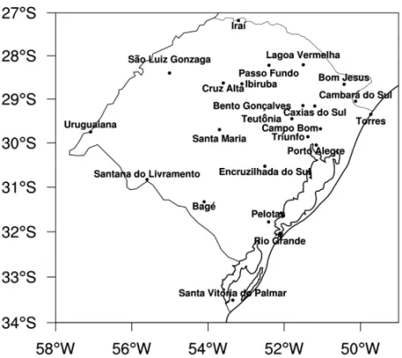
Figure 1 – Geographic distribution of the 23 weather stations over RS. Table 1 – Thresholds for each instability indices indicating atmospheric instability.

Index Skill scores References CAPE ≥ 1000 J/kg–1 Bluestein (1993)

CIN 0–50 J/kg–1 Houze (2014) LI and BLI ≥ –4 K or◦C Houze (2014) K ≥ 30◦_C _{Henry (1987)}

TT ≥ 40◦_C _{Nascimento (2005)}

some questions still arise: how good is instability indices to fore-cast rainfall, specially, extreme rainfall? What is the relationship between them? To trying assess such relationship seasonal corre-lations were calculated between each instability index and rainfall observed in the events selected.

Instability indices values from CFSR data were interpolated to weather stations coordinates, allowing Spearman Correlation Coefficient being computed for indices and rainfall for each loca-tion on RS. Statistical significance of Spearman correlaloca-tions was tested at 95% confidence level, using Fisher transformation. Cor-relation coefficients should be greater or equal to the seasonal critical values presented in Table 2 for being considered statisti-cally significant.

Table 2 – Critical correlation values for each season. Seasons n r critical JFM 31 0.301 AMJ 19 0.391 JAS 21 0.370 OND 34 0.287 RESULTS

Annual and Monthly Distributions of Extreme and Median Rainfall

Monthly mean percentiles of extreme rainfall events are show in Figure 2. It can be seen high extremes in October and November, higher than 70 mm. In later summer and earlier autumn events with 95 percentile values above 70 mm (outliers) are observed. On average, June is the only month with median less than 40 mm, showing that the majority of events has extreme rainfall above 40 mm.

A total of 105 events were identified as extreme and 342 as ordinary events in 2000-2009 period. Figure 3 shows the an-nual and monthly variation for these events. It is not possible to observe important trends in the frequency of extreme and median events in the studied period. There is, on the other hand, a mini-mum of events in 2001 for both groups of events. It could be as-sociated with La Ni˜na observed in 2000 and 2001. In the monthly distribution, there is no evidence for preference of occurrence of

(4)

Figure 2 – Monthly distribution mean 95 percentiles in extreme rainfall episodes for period 2000-2009. Circles indicate discrepant values.

Figure 3 – Annual (a) and monthly (b) distribution of the extreme rainfall (dark) and median (gray) events over RS, southern Brazil, from 2000-2009.

extreme and median events in any month. January and October have higher frequency of events.

Mean Characteristics Associates with Extreme Rainfall Events

This section presents seasonal composites fields for extreme rainfall events identified in 2000-2009 period. Sequences of composites are useful for tracking the evolution of the synoptic-scale systems responsible for extreme rainfall. Composites for autumn are presented in detail, since they showed remarkable differences in relation to median events. For other seasons, only noticeable differences from autumn events are presented.

Autumn: Composites fields for 500-hPa geopotential height are

shown in Figure 4a. It could be observed a decrease of spatial coverage of significant differences between extreme and median events from D-1 (not shown) to D0. However, there is an ex-tensive area of significant differences in sea level pressure west of RS for D0 (Fig. 4b), where a low-pressure center is present. This low-pressure center contributes to an increase of pressure

gradient over northeast Argentina and southern Brazil, which in turn establish an intense northerly flow. This northerly flow is commonly associated with transport of warm and moist air from Amazon basin to northern Argentina and southern Brazil.

Figure 5 shows the result of the increase of pressure gra-dient west of RS. Northerly flow covers great part of Brazil with significant differences to median events located over almost en-tire southern Brazil. These intense northerly winds speeds (greater than 18 ms–1_{over Paraguay, Bolivia, and state of Mato Grosso do}

Sul, Brazil), as already mentioned, bring moisture from Amazon basin which converge over RS.

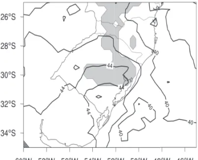
Composites fields for 200-hPa wind divergence, 850-hPa temperature advection and 500-hPa relative vorticity advection (not shown) did not present any significant differences between extreme and median events. It appears these parameters are not good precursors to the occurrence of extreme rainfall. When in-stability indices were analyzed, only K and TT presented signifi-cant differences. Although composites shown in Figure 6 present values indicative of atmospheric instability (see Table 1) over al-most entire domain, the differences between extreme and ordinary

(5)

i i

“main” — 2018/2/6 — 19:27 — page 135 — #5

i i

135

Figure 4 – 500-hPa geopotential height (mgp) composite (a) and SLP (hPa) (b) referring to D0 for autumn. Shaded areas are significant at 95% level.

Figure 5 – As Figure 4, but for meridional wind (m/s) at 850 hPa (a) and moisture flux divergence (10–7s–1) (b) referring to D0.

events are small over RS. Instability indices also do not seem to be good precursors for extreme rainfall.

Intraseasonal Differences

Winter: Magnitude of significant differences between extreme

and ordinary events for 500-hPa geopotential height are similar to autumn season. However, a more pronounced trough east of Andes is observed (Fig. 7a). Strong pressure gradient, especially on RS is also observed, but it seems to be a common feature for both extreme and ordinary events (Fig. 7a). It is interesting to note that northerly flow speeds increase from D-1 to D0 over boundary between Brazil, Bolivia and Paraguay. Again, as seen in mean sea level pressure, this northerly flow does exist in both set of events

(Fig. 8). Indices K and TT (not shown) have presented typical val-ues for storms, but there were not significant differences between extreme and ordinary events.

CAPE (independent of starting level; see Methodology) does not indicate high potential for convection, since maximum value was about 650 J/kg–1_{over Argentina, Uruguay and RS.}

How-ever, one should remember that composites have an inclination to smooth the results. Also, these fields are related to 12 UTC, or 09 local time. High potential to convection, what means high values of CAPE (see Table 1), is often seen during afternoon, but not in the morning. Nevertheless, it can be assumed that there is a small potential to convection, since significant differences areas were observed, showing that extreme rainfall events are somewhat distinct from ordinary ones (Fig. 9a). CAPE and CIN were also

(6)

Figure 6 – As Figure 4, but for K (a) and TT (b) (◦C), referring to D0.

Figure 7 – As Figure 4, but to 500-hPa geopotential height (mgp) (a) and SLP (hPa) (b) referring to D0 for winter.

(7)

i i

“main” — 2018/2/6 — 19:27 — page 137 — #7

i i

137

Figure 9 – As Figure 4, but to CAPE 255 (a) and CIN 255 (b) (J/kg) referring to D0 for winter.

observed over some areas near RS (Fig. 9b). According to Nasci-mento (2005), presence of CIN in unstable environments can in-crease the chance of occurrence of deep convection due forma-tion of a few convective cells, reducing competiforma-tion for CAPE and increase the duration of convection.

Spring: 500-hPa geopotential height differences for autumn are

the largest among all seasons. Although there is not a pronounced trough at middle levels of troposphere, the differences between extreme and ordinary events are spatially extensive and have a small increase between D-1 and D0 (Fig. 10). This configura-tion provides a stronger pressure gradient (in relaconfigura-tion to ordinary events) observed since two days prior extreme rainfall (Fig. 11). With a stronger gradient pressure, stronger northerly flow is ob-served over a large area of southern South America, bringing moisture to RS (Fig. 12).

Summer: Composite fields for summer were smoother than

those for other seasons, especially 500-hPa geopotential height. Although composites of sea level pressure were not significantly different and northerly flow less intense when compared with other seasons, they are presented in Figure 13, since configuration showed in these fields helped modulate conditions for rainfall. For K index, it can be seen again, RS covered by values indicative of atmospheric instability, but only a small area shows differences between extreme and ordinary events (Fig. 14).

Relation Between Extreme Rainfall and Instability Indices

The mean characteristics of atmosphere shown above present how atmosphere organizes itself to produce an extreme rainfall event. It could be seen some indication of instability by instability

(8)

Figure 11 – As Figure 4, but to SLP (hPa) referring to D-2 (a), D-1(b) and D0 (c), respectively, for spring.

Figure 12 – As Figure 4, but to meridional wind (m/s) at 850 hPa (a) and moisture flux divergence (10–7s–1) (b), referring to D0 for spring.

(9)

i i

“main” — 2018/2/6 — 19:27 — page 139 — #9

i i

139

Figure 14 – As Figure 4, but to K index (◦C), referring to D0 for summer.

Table 3 – Summary of correlations between instability indices and cases of extreme rain.

JFM AMJ JAS OND

D-2 D-1 D0 D-2 D-1 D0 D-2 D-1 D0 D-2 D-1 D0 *N *C N C+ N C+ N C+ N C+ N C+ N C+ N C+ N C+ N C+ N C+ N C+ N CAPE solo 15 0.56 2 0.58 18 0.60 14 0.72 10 0.61 11 0.74 14 0.64 19 0.83 9 0.71 17 0.54 11 0.48 14 0.54 CAPE 255 17 0.59 4 0.58 20 0.59 6 0.55 7 0.63 12 0.63 10 0.59 14 0.62 10 0.61 12 0.51 9 0.47 21 0.53 CAPE 180 20 0.60 4 0.56 20 0.57 6 0.55 5 0.63 16 0.63 12 0.62 12 0.62 11 0.62 10 0.51 10 0.46 20 0.54 CAPE 90 19 0.64 4 0.54 19 0.56 12 0.72 12 0.61 14 0.76 18 0.78 17 0.72 16 0.63 15 0.58 13 0.56 20 0.57 CIN 255 17 0.54 11 0.57 14 0.63 13 0.58 13 0.59 6 0.61 13 0.62 8 0.59 9 0.55 11 0.56 15 0.54 15 0.56 CIN 180 16 0.53 12 0.59 15 0.62 12 0.59 13 0.61 6 0.56 15 0.63 8 0.58 5 0.56 11 0.58 16 0.54 13 0.57 CIN 90 17 0.62 10 0.60 13 0.61 17 0.60 16 0.70 10 0.60 18 0.81 13 0.71 14 0.68 15 0.66 22 0.60 11 0.54 K 14 0.53 6 0.65 17 0.59 9 0.57 5 0.54 9 0.58 7 0.53 5 0.46 7 0.53 11 0.47 7 0.51 11 0.56 TT 13 0.51 12 0.68 15 0.63 10 0.58 8 0.48 9 0.56 8 0.51 7 0.54 7 0.55 11 0.52 9 0.52 8 0.53

*N – Number of weather stations with significant correlation in the state-RS. *C+ – Greater value significant correlation observed in state-RS.

indices. But, are instability indices a good indicator for extreme rainfall? To address this question correlation between extreme rainfall and instability indices was analyzed. Only most significant correlations (see Table 3), for each season are shown.

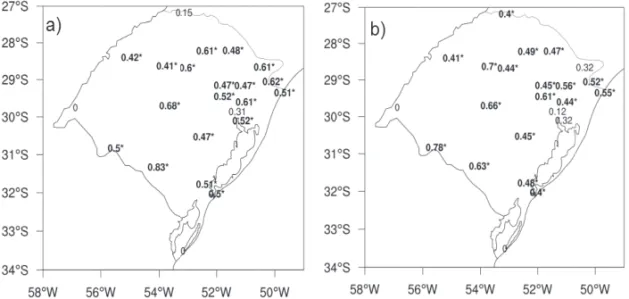
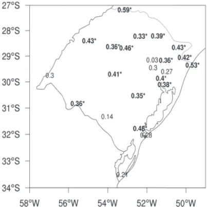
Autumn: Figure 15 and 16 show Spearman correlations for

CAPE ground, CAPE 90 and CIN 90, respectively, which present more significant correlation with extreme rainfall in autumn. For CAPE ground, two days prior rainfall almost entire RS area has statistically significant correlations, being on average above 0.50. From D-2 to D0 a decrease in the number of weather stations with significant correlation is observed, so the mean correlation over RS (Table 2). CAPE 90 and CIN 90 have similar spatial coverage

of significant correlation, as well as almost same mean correla-tion over RS. CAPE 255 and CAPE 180 displayed more important correlations only on D0 (not shown). For K and TT indices only 9 weather stations were significant between D-2 to D0 (not shown).

Winter: Again, CAPE ground and CAPE 90 present a large

number of weather stations with significant correlation, show-ing correlations higher than 0.80 and 0.75, respectively, slightly higher than observed in autumn (Fig. 17). Also, spatial coverage of significant correlation maintained almost fixed from D-2 to D0 (Table 3).

CAPE obtained from other start levels (CAPE 255 and CAPE 180; not shown) also presents significant correlation with

(10)

Figure 15 – Rank correlation coefficient between CAPE ground and extreme rainfall on D-2 (a) and D0 (b). The fields are

dimen-sionless, and values in bold marked with an asterisk show significant correlation.

Figure 16 – As Figure 15, but to CAPE 90 on D0 (a) and CIN 90 on D-1 (b).

(11)

i i

“main” — 2018/2/6 — 19:27 — page 141 — #11

i i

141

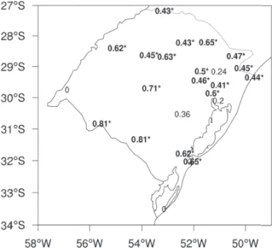
extreme rainfall, with maximum value of 0.62 and 13 weather stations with significant correlation. CIN 90 presents high cor-relations (above 0.7) two days prior extreme rainfall (Fig. 18). K and TT indices (not shown) had significant correlations, but with relatively small values as compared with autumn.

Figure 18 – As Figure 15, but to CIN 90 on D-2 for winter.

Spring: Correlations for CAPE at all starting levels had broader

spatial coverage of significant correlation than autumn and win-ter seasons. CAPE 255, for example, has only 2 weather stations with non-significant correlations with rainfall (Fig. 19a). CIN 90 presents high spatial coverage of significant correlation and a maximum of 0.7 a day prior to extreme event (Fig. 19b). A de-crease in the number of weather stations with significant corre-lation is observed for CIN 90 and CIN 255 (Table 3). K and TT indices, had about 10 weather stations significantly correlated (not shown). Even though amount of significant weather stations was larger than observed in autumn and winter, maximum values were not higher.

Summer: CAPE indices were similar to those observed in spring

(Table 3). CAPE ground and CAPE 255 were more significant a day prior extreme rainfall, with almost all weather stations having significant correlations, to CAPE 180 and CAPE 90 were more important on D-2 (not shown). CIN 255 presents significant cor-relations with larger spatial coverage than autumn on D-0, show-ing similarities with sprshow-ing season (Fig. 20). Correlations between K and TT indices with extreme rainfall were more significant than in other seasons (Fig. 21), with K showing a huge increase in the number of weather stations with significant correlations: 6 on D-1 to 17 on D0. TT index does not show large variations

in number of significant weather stations between days prior to rainfall and D0.

DISCUSSION

In this investigation, very low values for CAPE, compared with thresholds for strong convection, were observed in all seasons. These results can indicate that extreme rainfall events did not have strong relationship with CAPE. However, it is important to remem-ber that composite fields are related to variables averaging and also they refer to 12 UTC, which is 9 local time. All of it can con-tribute to attenuated CAPE values here observed. Tavares & Mota (2012) also found smaller values of CAPE when dynamic forcing was more intense, as compared with cases in which rainfall events depended on thermodynamic forcing for convective development. Some studies pointed the importance of dynamic forcing for break instability conditions (presence of high values of CIN), what favors occurrence of convection (Foss, 2011; Hallak, 2012). In addition, some studies found high values of CAPE before precipitation and a decreasing during or after its occurrence (Tavares (2009, 2010); Tavares & Mota, 2012). In this study, increase of CAPE occurs from D-1 to D0, corresponding to the beginning of daily rainfall accumulation (daily rainfall is recorded from 12 UTC of one day to 12 UTC of following day, being assigned as rainfall of the later). It is expected to observe a decrease of indices values if compos-ites were extended up to a day after extreme event, as discussed by Tavares (2009). This author argues that this decrease occurs be-cause cold air descending from cloud base, accompanying rain-fall, contribute to diminish the temperature between cloud base and surface, leaving this part of atmosphere more stable.

The results of this study emphasize a discussion related to instability indices for Brazil, especially when they are used for rainfall forecasting. As shown above, lower values of CAPE are associated with extreme rainfall occurrence, what is highly linked to severe convection. Maybe, lower values of CAPE, as com-pared with thresholds shown in Table 3, may be sufficient for occurrence of severe convection, as discussed by Nascimento (2005). It is important to emphasize that instability indices are diagnostic tools for thermodynamic instability of atmosphere, but not for rainfall. Correlations between instability indices and ex-treme rainfall showed statistically significant linear relationship. It was also observed that some indices such as CAPE, for exam-ple, when calculated from a level above ground, have higher re-lationship with observed rainfall. This result is important, since may help meteorologists in correctly identify a potential envi-ronment for severe convection and, consequently, for extreme rainfall. It is common in weather forecasting centers the use of

(12)

Figure 19 – As Figure 15, but to CAPE 255 on D-0 (a) and CIN 90 on D-1 (b) for spring.

Figure 20 – As Figure 15, but to CIN 255 referring to D0 for summer.

instability indices calculated only from ground level, where not always is the level of higher instability. However, except for a few observations, the great majority of correlations for all sea-sons had values between 0.4 and 0.5. The variability of a vari-able represented by another varivari-able is, in this study therefore, between 16 and 25%, approximately. It is shown, quantitatively, what it is empirically observed daily in forecasting centers about the task of predicting rainfall with instability indices. On the other words, the degree of convective instability of atmosphere has a very low correlation, although statistically significant, with

the amount of rainfall observed. Thus, although results in Ta-ble 3 are an attempt to associate the magnitude of instability in-dices to rainfall amount, they have a very small contribution to quantitative rainfall forecasting. As mentioned above, there are situations in which convective potential is below the thresholds presented in Table 3, but large amount of rainfall is still observed. The methodology here used may impacted the results, but they agree with empirical knowledge of forecasters. However, it is not a suggestion to exclude instability indices from operational rou-tines, but emphasizes that they should be used for what they were

(13)

i i

“main” — 2018/2/6 — 19:27 — page 143 — #13

i i

143

Figure 21 – As Figure 15, but to K (a) and TT (b) indices (◦C), referring to D0 for summer.

created: to describe the convective potential of atmosphere. The quantitative rainfall forecasting should use these and other tools, since many factors may contribute to rainfall occurrence and in-tensity. Also, it should be noted that there are no “magic numbers” to forecast these events, as discussed in Nascimento (2005) and Doswell & Schultz (2006). This is a task of meteorologists to use available information and their experience for a better understand-ing of atmosphere behavior and for a better weather forecastunderstand-ing.

CONCLUSION

The purpose of this study is to evaluate the relationship between instability indices and extreme rainfall occurred in RS, Brazil. In addition, the search for forerunning synoptic-scale features as-sociated with these extreme rainfall events. Based in compos-ites for up to 2 days before extreme rainfall events, it could be observed how different they are comparing to ordinary rainfall events. Some common features observed in all season were: (i) formation of a surface thermal low pressure center in northern Argentina and Paraguay, (ii) intensification of northerly winds over Bolivia, Paraguay and northern Argentina, responsible for warm and moist air transportation for southern Brazil. This more intense northerly flow is associated with an increase of pressure gradient over the regions cited in (i). It was also observed (iii) moisture flux convergence over eastern Paraguay, northern Argentina and southern Brazil, especially over RS.

Correlations between instability indices and extreme rainfall showed statistically significant linear relationship for almost all indices. However, they did not show anticipated indication of rainfall occurrence, and also confirm what is empirically known:

instability indices are bad tools to forecast rainfall. Quantitative rainfall forecasting should be performed by meteorologists using a set of tools and information. Instability indices can help mete-orologists to identify atmospheric environments favorable to ex-treme convection, but they say nothing about amount of rainfall that can be observed in a forthcoming event.

REFERENCES

BLUESTEIN HB. 1993. Synoptic dynamic meteorology in midlatitudes: observations and theory of weather systems. New York: Oxford Univer-sity Press, 594 pp.

CAVALCANTI IFA. 2012. Large Scale and Synoptic Features Associated with Extreme Precipitation over South America: A Review and Case Stud-ies for the First Decade of the 21st Century. Atmos. Res., 118: 27–40, doi:10.1016/j.atmosres.2012.06.012.

DOSWELL CA III & SCHULTZ DM. 2006. On the use of indices and pa-rameters in forecasting severe storms. EJSSM, 1(3): 1–22.

FOSS M. 2011. Condições atmosféricas conducentes à ocorrência de tempestades convectiva severas na América do Sul. Master Dissertation on Meteorology, Programa de Pós-Graduação em Meteorologia, Univer-sidade Federal de Santa Maria, Brazil, 2011. 145 pp.

GRIMM AM. 2009. Clima da regi˜ao sul do Brasil. In: CAVALCANTI IFA, FERREIRA NJ, SILVA MGAJ & DIAS MAFS (Org.). Tempo e Clima no Brasil. S˜ao Paulo: Oficina de Textos, p. 259–275.

HALLAK R. 2012. CAPE e CINE – Apostila Meteorologia F´ısica I. Avail-able on:<http://www.dca.iag.usp.br/www/material/>. Access on: Jan. 27, 2015.

(14)

parâmetros convectivos e modelos de mesoescala: uma estratégia ope-racional adotável no Brasil? Rev. Bras. Meteorol., 20: 121–140. RAO VB & HADA K. 1990. Characteristics of rainfall over Brazil: annual variations and connections with southern oscillation. Theor. Appl. Cli-matol., 42: 81–91.

RASMUSSEN KL & HOUZE RA. 2016. Convective Initiation near the Andes in Subtropical South America. Mon. Wea. Rev., 144: 2351–2374, doi: 10.1175/MWR-D-15-0058.1.

RASMUSSEN KL, ZULUAGA MD & HOUZE RA. 2014. Severe Convec-tion and Lightning in Subtropical South America. Geophys. Res. Lett., 41: 7359–7366, doi:10.1002/2014GL061767.

REBOITA MS, KRUSCHE N, AMBRIZZI T & ROCHA RP. 2012. Entenden-do o tempo e o clima na Am´erica Entenden-do Sul. Terrae Didat., 8(1): 34–50. SAHA S, MOORTHI S, PAN HL, WU X, WANG J, NADIGA S, TRIPP P, KISTLER R, WOOLLEN J, BEHRINGER D, HAIXIA L, STOKES D, GRUMBINE R, GAYNO G, WANG J, HOU YT, CHUANG H, JUANG HMH, SELA J, IREDELL M, TREADON R, KLEIST D, DELST PV, KEYSER D, DER-BER J, MICHAEL E, MENG J, WEI H, YANG R, LORD S, DOOL H, KUMAR A, WANG W, LONG C, CHELLIAH M, XUE Y, HUANG B, SCHEMM JK, EBISUZAKI W, LIN R, XIE P, CHEN M, ZHOU S, HIGGINS W, ZOU CZ, LIU Q, CHEN Y, HAN Y, CUCURULL L, REYNOLDS W, RUTLEDGE G &

GOLD-TAVARES JPN & MOTA MAS. 2012. Condição termodinâmica de eventos de precipitação extrema em Belém-PA durante a estação chuvosa. Rev. Bras. Meteorol., 27: 207–218.

TEDESCHI RG, GRIMM AM & CAVALCANTI IFA. 2014. Influence of Central and East ENSO on extreme events of precipitation in South America during austral spring and summer. Int. J. Climatol., doi:10.1002/joc.4106.

TEIXEIRA MS. 2010. Caracterização f´ısica e dinâmica de episódios de chuvas intensas nas regiões sul e sudeste do Brasil. PhD Thesis on Meteorology, Programa de Pós-graduação em Meteorologia, Instituto Nacional de Pesquisas Espaciais, São José dos Campos, Brazil, 2010. 190 pp.

VELASCO I & FRITSCH JM. 1987. Mesoescale convective complexes in the Americas. J. Geophys. Res., 92: 9591–9613.

WILKS DS. 2006. Statistical Methods in the Atmospheric Sciences. 2nd ed., International Geophysics Series, vol. 91, Academic Press, 627 pp.

ZIPSER EJ, CECIL DJ, LIU C, NESBITT SW & YORTY DP. 2006. Where are the Most Intense Thunderstorms on Earth? Bull. Amer. Meteor. Soc., 87: 1057–1071, doi:10.1175/BAMS-87-8-1.

Recebido em 21 maio, 2015 / Aceito em 30 novembro, 2016 Received on May 21, 2015 / Accepted on November 30, 2016