Abstract— We present a methodology of parametric objective function coefficient programming for large linear programming (LP) problem. Most of current parametric programming methodologies are based on the assumption that the optimal solution is available. Large linear programming problems in real-world might have millions of variables and constraints, which makes it difficult for the LP solver to return the optimal solutions. This paper extends the traditional parametric programming methodology by considering features of the large LP problems. By considering the tolerance of infeasibility and introducing a step size to deal with degeneracy of the problem, the parametric objective function coefficient linear programming of large LP problem can be conducted while the optimal solutions are not available. Experiment results of LP problems with different scales are provided.
Index Terms—linear programming, large problem, simplex-based, parametric programming
I. INTRODUCTION
inear programming(LP) is widely used in the industrial system. Analyzing impact of parametric setting on the
solution of interested variables is helpful to the improvement of the model and the explain-ability of the solution. A lot of trial-and-error to obtain the desired solution by changing parameters is time consuming, while sensitivity analysis[1] and parametric programming can help about this.
The simplex-based parametric programming methodology was first provided by Gass and Saaty [2] in 1955. By taking advantage of the iterations in simplex algorithm, this methodology tries to find the parametric interval in which the current optimal basis stays optimal. Degeneracy could not be handled in this methodology. New approaches like interior point based [3], [4], support sets based [5] methodology were proposed in the last decades. The concept of optimal partition was introduced into the interior point based parametric programming. Most of them are based on the assumption that strictly complementary solution is available. However, it’s hard for LP solver to get the optimal solution of large LP problems because of the time and precision limitation, so that those parametric programming methodologies are no longer applicative.
Manuscript received January 7, 2012; revised January 28, 2012. This work was supported in part by the Intel.
Huang,Rujun is with the Southwest Jiaotong University, ChengDu, SiChuan, China. E-mail: rjhuang1201@ gmail.com.
Lou,Xinyuan is with the Southwest Jiaotong University, ChengDu, SiChuan, China. E-mail: [email protected].
This paper extends the traditional simplex based parametric programming methodology to adjusting the objective function coefficient parameters of the large LP problem. The main idea to conduct the parametric programming is to preserve the current optimal basis, optimal partition or support set [5] while the parameters are changing. We provide a new definition of the optimal of the current optimal basis in the parametric programming iterations.
II. PROBLEM DEFINITION
The linear programming problem can be defined as:
Min C X C X
Subject to A X A X B
LB X UB (1)
Where
C /C : The objective function coefficient of decision variables in/out of the basis
A /A : The constraint coefficient matrix of decision variables in/out of the basis
B: The right hand side value vector
LB/UB: The lower bound/upper bound of decision variable vector X
X /X : The decision variable vector in/out of the basis
B/N A set contain the indices of variable in/out of the basis
Given the parameter θ, the objective function coefficient can be denoted by C C0 fun θ , where C0 is the current
objective function coefficient and the fun θ here presents the perturbation vector. The parametric programming on objective function coefficient will observe the behavior of solution with respect to the change of θ.
III. SIMPLEX BASED PARAMETRIC PROGRAMMING
In this section, we introduce the simplex based parametric programming. The reduced cost for non-basic variables in
the optimal solution of this problem can be defined as:
RC C A A C j ∈ N (2) Introducing θ into the reduced cost function yield:
RC θ C fun θ A A C fun θ
C A A C A A fun θ fun θ
j ∈ N (3)
We restrict the objective function coefficient to be a linear function of θ. The function of the coefficient can be denoted as Cj Cj′ θ , j∈ B,N , we have
A Simplex Based Parametric Programming
Method for the Large Linear Programming
Problem
Huang, Rujun, Lou, Xinyuan
RC θ C A A C C′ A A C′ θ, j ∈ B, N (4)
RC θ can be simplified as:
a b θ, j ∈ N (5) Where
a C A A C , j ∈ N (6)
b C′ A A C′ , j ∈ N (7) a: The reduce cost of the non-basic variables in the current optimal solution.
b : The variation of reduced cost by increasing one unit of θ based on the current basis.
The interval of the θ in which the current optimal basis remains optimal is determined by keeping the reduced cost of non-basic variables non-negative: RCj θ 0 .
The lower bound and the upper bound of θ in which the current optimal basis will stay optimal are denoted by LBP1
and UBP1, respectively.
LBP max , when b 0
Inf, when b 0 , j ∈ N
UBP max , when b 0
Inf, when b 0 , j ∈ N (8)
This methodology works well only if the LP model is non-degenerate and the optimal solution is available.
If the LP model is non-degenerate, we would have LBP1 0 and UBP1 0 , since aj 0 in the
non-degenerate minimizing problem. So that we have LBP1 UBP1 and a new interval in which the current basis will
keep optimal of the parameter is obtained.
But if the problem is dual degeneracy [6], the reduced cost for some of the non-basic variables might be zero. So we might have LBP1 UBP1 0 , which means the
current basis will remain optimal only if the parameter keeps the current value.
There are several features for large LP problem:
1) It’s hard to have both the primal infeasibility and dual infeasibility equal to zero in the final basis because of the time and precision limited, which means that the optimal solution is usually not available.
2) Based on the point above, Solution within certain tolerance is acceptable and same extent of accuracy loss is allowed.
In large-scale LP problems, there might be invalid reduced costs or bound violations for some variables when the LP solver reaches its optimum. There is actually a gap between the optimal solution and the final solution returned by LP solver. It is hard to find a parameter interval, in which the solution will keep optimal by this methodology.
IV. PARAMETRIC PROGRAMMING ALGORITHM FOR LARGE LP MODEL
Considering the problems above, we provide a methodology to conduct parametric programming on large LP problem by extending the methodology above. In this methodology of parametric objective function coefficient linear programming, selective pre-processing is conducted
to remove the fixed variables and redundant constraints of the LP model before the parametric programming. Primal and dual infeasibility are used as criterions of the optimal of the LP model in the calculation of the parameter intervals. In order to move forward in the parametric programming calculation, a step size variable is introduced. If stalling is encountered, we will change the current parameter value by the step size in order to skip the stalling point.
A. Pre-processing
Pre-processing is used to simplify the problem. The size of problem after pre-processing is reduced by aggregating variables and constraints, eliminating redundancy and so on. Taking advantage of pre-processing seems like a good idea to reduce the number of degenerate variables and the size of LP problem since some of the degeneracy of the model might be caused by the redundant constraints. However, pre-processing picks out redundant constraints and variables; these constraints and variables are redundant in the original LP model, but they might not be redundant in the LP model with changed parameters. The change of objective coefficients has no impact on the fixed variables the redundancy of constraints. Then fixed variables and redundant constraints can be ignored when we change the objective coefficients.
B. Parametric objective function coefficient Programming
In the traditional simplex based parametric objective coefficient programming, the parameter interval is determined by ensuring the reduced cost still satisfy the optimal condition, so that the current basis will stay optimal in the whole interval. But there might be some invalid reduced cost in the final optimal solution of the problem returned by the LP solver. Here we redefine the optimum of the solution. It’s reasonable to take the max reduced cost infeasibility (MRCI or dual infeasibility) as the validation the optimum of the optimal basis in the last iteration in parametric objective function coefficient programming because of the three points below:
1) The primal infeasibility for the current basis will keep the same no matter how we vary the parameters in the objective function coefficient.
2) By keeping the MRCI no greater than the current optimal solution, we would have both of the primal infeasibility and dual infeasibility no greater than the value returned by the LP solver in the last parametric programming iteration.
3) There is at least one parameter value (the current parameter value) meets the infeasibility tolerance.
We take the MRCI as the criteria to determine if the current solution can be accepted as the optimal solution in the parametric objective function coefficient linear programming.
Here CBV′ and CNV′ are objective coefficient increment for
Cj Cj′ θ ,j∈B∪N
Define the amount of the parameter increment as UPW and the step size for skipping stalling as PS. Similar algorithm can be employ while the parameter decreases.
Step1: Do selective preprocessing to remove the fixed
variables and redundant constraints. Standardize the model. Primal problem:
Min:CX
Subject to: AX B
X 0 (9) Dual problem:
Max:BY
Subject to: ATY C (10)
Step2: Optimize the problem and calculate the aj and bj
in (6) and (7). Go to step 4.
Step3: Solve the problem with LP solver starting with
the current basis and the new objective coefficient, and get the new optimal solution, aj and bj in Cj θ .
Step4: If the reduced cost meets the optimal condition,
calculate the upper bound: UBP1 in (8). Else go to step5. A new interval is obtained;
UBP Max UBP1,UPW , UBP1 0
PS, UBP1 0
(11) If θ is equal to UPW , the parameter reaches the upper bound we provided, then stop, else go to step6
Step5: Calculate the max reduced cost
infeasibility MRCI for all the dual constraints for the current optimal basis.
MRCI
max AjTY Cj when AjTY Cj 0 , ∈ 1,
0,when AjTY Cj 0 , ∈ 1,
(12)
If we keep the current basis, the max reduce cost infeasibility might change with respect to the change of parameter. The dual constraints can be denoted by:
AT ai bi θ C0j θ Cj′,i∈M ,j∈N (13) The dual infeasibility of some constraints might increase while some might decrease when the parameter value is increasing. What we have to make sure is that the Maximum dual infeasibility for the current basis is within the tolerance Tol or no less than the current value Cur_MRCI in the parameter interval.
The upper bound and lower bound of θ can be fixed as follows:
MRCI max Tol ,Cur_MRCI
min C0j ATai Cj′ bi θ MRCI, when AT ai bi θ C0j θ Cj′, j ∈N (14)
LBP2
max MRCI C0j A
T
ai
Cj′ bi ,
when Cj′ bi 0
INF,when Cj′ bi 0
(15)
UBP2 min
MRCI C0j ATai
Cj′ bi ,
when Cj′ bi 0
INF,when Cj′ bi 0
(16)
UBP Max UBP2,UPW ,UBP2 0
PS,UBP2 0 (17) If UBP is equal toUPW, the parameter reaches the upper bound we provided, then stop, else go to step6
Step6: Increase the objective coefficient C through
C C UBP C′ (18) UPW UPW UBP (19)
V. NUMERICAL EXAMPLES
We take the CPLEX as the LP solver and conduct parametric programming on the supply chain linear programming problems with different size by changing the same weight.
The experiments provide two of the decision variable values we interested in while the weight which impacts the objective function coefficient of multiple variables is increasing from the current value to the target value.
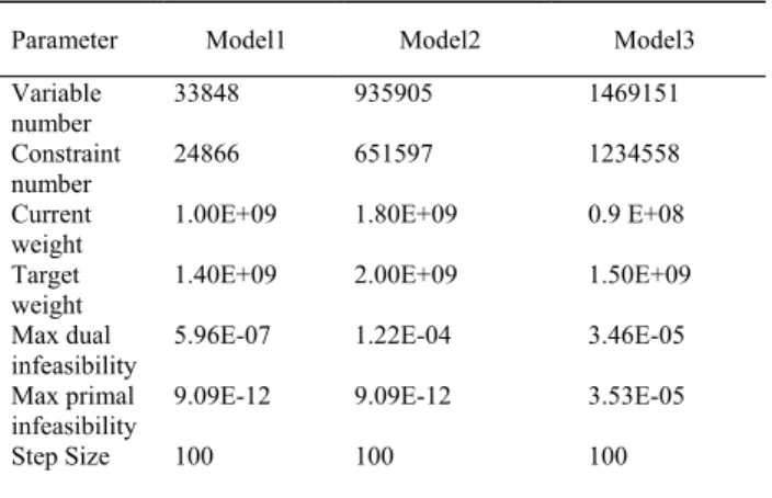
The parameters of the three models in experiments are
provided in Table I. Fig.1 to Fig.3 provide the solution of two decision variables: , and the corresponding infeasibility.
From the solution of the three models above, the dual infeasibility and primal infeasibility of the final solution returned by the LP solver are increasing while the size of the model is increasing. Since the parameter intervals are determined by making sure the primal and dual infeasibility no greater than the last solution returned by the LP solver. In each interval without using the step size, the dual infeasibility and primal infeasibility will keep no greater than the infeasibilities in corresponding parameter interval provided by the second part of figures above.
The step size set to 100, which is much less than the total interval length (gap between target weight and current weight). In this algorithm, the decision variable values and infeasibilities are undefined in the parameter intervals in which the step size is using.
TABLE I EXPERIMENTS PARAMETERS
Parameter Model1 Model2 Model3
Variable number
33848 935905 1469151
Constraint number
24866 651597 1234558
Current weight
1.00E+09 1.80E+09 0.9 E+08
Target weight
1.40E+09 2.00E+09 1.50E+09
Max dual infeasibility
5.96E-07 1.22E-04 3.46E-05
Max primal infeasibility
9.09E-12 9.09E-12 3.53E-05
Fig. 1(a) Solutions of , of Model 1 Fig. 2(b) Primal and dual infeasibility of Model 2
Fig. 1(b) Primal and dual infeasibility of Model 1
Fig. 2(a) Solutions of , of Model 2
Fig. 3(a) Solutions of , of Model 3
VI. CONCLUSION
Parametric programming can provide the behavior of related decision variables values with respect to the variations of the parameter. For the large linear programming problems, the traditional parametric programming theory could not be applied to problem directly since the optimal solution is not always available. By considering the tolerance of infeasibility, we employ the parametric objective function coefficient programming on large linear programming problems. Step size is introduced to deal with the degeneracy. If stalling is encountered because of degeneracy, some of the parameter intervals will be discrete.
REFERENCES
[1] James E.Ward, Richard E.Wendell, “Approaches to sensitivity analysis in linear programming,” Annals of Operations Research, vol.27, pp.3-38, 1990.
[2] S.I.Gass, T.L.Saaty,. “The computational algorithm for the parametric objective function Naval Research Logistics Quarterly,” vol.2, pp.39-45, 1955.
[3] B. Jansen, C. Roos,T, Terlaky, “An interior point approach to post optimal and parametric analysis in linear programming”. The Faculty of Technical Mathematics and Informatics
[4] Ilan Adler, Renato D. C. Monteiro, “A geometric view of parametric linear programming.” Algorithmica, vol.8, pp.161-176, 1992. [5] Milan Hladik, “Multi-parametric linear programming: Support set and
optimal partition invariance,” European Journal of Operational Research, vol.202, pp.25-31, 2010.