Fitting and testing the significance of linear trends in Gumbel-distributed data

Fitting and testing the significance of linear trends in

Gumbel-distributed data

Robin T. Clarke

Instituto de Pesquisas Hidráulicas,UFRGS Porto Alegre, RS Brazil

Email:Clarke@iph.ufrgs.br

Abstract

The widely-used hydrological procedures for calculating events with T-year return periods from data that follow a Gumbel distribution assume that the data sequence from which the Gumbel distribution is fitted remains stationary in time. If non-stationarity is suspected, whether as a consequence of changes in land-use practices or climate, it is common practice to test the significance of trend by either of two methods: linear regression, which assumes that data in the record have a Normal distribution with mean value that possibly varies with time; or a non-parametric test such as that of Mann-Kendall, which makes no assumption about the distribution of the data. Thus, the hypothesis that the data are Gumbel-distributed is temporarily abandoned while testing for trend, but is re-adopted if the trend proves to be not significant, when events with T-year return periods are then calculated. This is illogical. The paper describes an alternative model in which the Gumbel distribution has a (possibly) time-variant mean, the time-trend in mean value being determined, for the present purpose, by a single parameter βestimated by Maximum Likelihood (ML). The large-sample variance of the ML estimate is compared with the variance of the trend β_LR calculated by linear regression; the latter is found to be 64% greater. Simulated samples from a standard Gumbel distribution were given superimposed linear trends of different magnitudes, and the power of each of three trend-testing procedures (Maximum Likelihood, Linear Regression, and the non-parametric Mann-Kendall test) were compared. The ML test was always more powerful than either the Linear Regression or Mann-Kendall test, whatever the (positive) value of the trend β; the power of the MK test was always least, for all values of β.

Keywords: Extreme value probability distribution, Gumbel distribution, statistical stationarity, trend-testing procedures

Introduction

Much hydrological and meteorological practice is concerned with the analysis of extremes. Four examples of variables used in such analyses are (a) annual maximum discharge in rivers; (b) annual minimum mean 10-day flows; (c) annual maximum rainfall intensities over 5-minute, 10-minute, .... durations; (d) annual extreme wind velocities. Analyses of such variables form the basis of important decisions in engineering practice (NERC, 1975), urban planning, and the calculation of insurance risks, the objective being to calculate the frequency of occurrence of extreme events. Central to many such analyses is the use of observed sequences of annual maxima (or minima) to fit an appropriate Extreme Value (EV) probability distribution, which can then be used to calculate the “return period” of extreme events (Stedinger et al., 1993). It is commonly assumed in all such analyses that the sequence of observed annual maxima (minima) is stationary, with each observation in the sequence drawn from an underlying EV distribution

that remains constant over time. But if changes in climate (Vinnikov et al., 1990; Guttman et al., 1992; Groisman and Easterling, 1994; Changnon and Kunkel, 1995; Olsen et al., 1999; Douglas et al., 2000), or in land use (Bruijnzeel, 1990, 1996; Sahin and Hall, 1996), result in gradual changes in the observed sequence, the assumption that the underlying EV distribution remains constant becomes invalid, and the task of predicting the frequency with which extreme events will occur in the future becomes very much more complicated. Furthermore, the report “Climate Change 2001: Impacts, Adaptation and Vulnerability” by the Intergovernmental Panel for Climate Change (IPCC, 2001) warns of climate change over the next century, envisaging “changes in the variability of climate, and changes in the frequency and intensity of some climate phenomena.” Such forecasts, now being made with ever-increasing confidence, imply that the statistical stationarity necessary for many hydrological analyses can no longer be assumed safely, and the spatial and temporal availability of water resources must

^ βMR

be expected to change as and when regional climate changes. This is of crucial importance to a developing country like Brazil, in which more than 90% of its energy is provided by hydropower.

This paper is concerned with some aspects of the detection and estimation of ”changes in the frequency and intensity of some climate phenomena” referred to in the above quote from the IPCC report. Two typical procedures for detecting whether trend exists in a sequence of annual extremes are (1) regression analysis (Salas, 1993), and (2) non-parametric methods, often by means of Mann-Kendall test (Hirsch et al.,1993). Neither method takes account of the facts that (a) where trend does not exist, hydrological and meteorological extremes can be expected to follow a distribution of EV type; (b) if trend does exist, it will be superimposed on data from an EV distribution. In the case of (1), data are assumed to be drawn from an underlying Normal distribution when trend is absent, whilst if trend is present, this Normal distribution is assumed to have time-variant mean. In the case of the Mann-Kendall test for trend, no explicit form for the underlying distribution is assumed, although where no trend is detected, it is common practice for a distribution of EV type then to be assumed for the purpose of estimating return periods of extreme events. Therefore, neither regression analysis nor Mann-Kendall tests are logically satisfactory when trend, if it exists, is superimposed on data from an EV distribution.

Two related papers (Clarke, 2002a, b) deal with the detection and estimation of trends in annual extremes of hydrological variables, where these are assumed, in the absence of trend, to follow Gumbel or Weibull distributions. The first paper casts the problem of estimating trend in data with underlying Gumbel distribution in the form of a Generalised Linear Model (GLM), and describes an iterative procedure for estimating trend parameters; the second paper modifies this iterative procedure to allow trends to be estimated, and tested for significance, in data with an underlying Weibull or a Generalised Extreme Value (GEV) distribution. The purpose of the present paper is to present an analytical result, and results of some simulations, that supplement and extend earlier results given for the Gumbel distribution; a second paper will present corresponding results for the Weibull distribution.

Although the emphasis of the present paper is on the estimation of trend in Gumbel-distributed data, the results have an important additional application in the analysis of sequences of Gumbel data in which no time-trends exist, but where it is required to explore relationships between a Gumbel variate and other, concomitant variables which may explain its behaviour. As an example, consider a sequence of annual maximum rainfall intensities each of one-hour

duration, with a (trend-free) Gumbel distribution; it may be of interest to relate the observed intensities to meteorological conditions – velocity and direction of wind – at the time at which each maximum intensity occurred. The approach given in this paper is relevant in this context also, the time-variate denoted by t simply being replaced by (for example) wind velocity V. The paper referred to above (Clarke, 2002a) extends the analysis to any number of concomitant variates.

Variance of regression estimate of

linear trend: data from a Gumbel

distribution

The case is taken where data in the absence of trend follow the Gumbel distribution

f_Y(y; u, a) = aexp[ – a (y – u) – exp { – a (y - u)}]

–

∞

∞

with mean u+ γ / a, variance π2_/6a2_{. With a linear trend}

superimposed, this distribution is modified to give

f_Y(y; u, a, b) = aexp[–a (y – u – b t ) – exp {–a (– u–b t)}] -

∞

∞

where t denotes time, so that the mean of the Gumbel random variable Y_t is (u+ γ/a) + b t. The constant γis Euler´s constant,

γ ≈ 0.57721... . Given N observations y₁, y₂, ...y_Nof Y at times t =t₁, t₂, ... t_N, the parameter βin (1a) is to be examined, to determine whether its magnitude warrants rejection of the hypothesis H₀: β = 0 in favour of the alternative H₁:

β≠ 0.

When βis estimated by linear regression to give

LR

^

β

∑

∑

i i

i i

i t t t t

y _ _ 2

) ( / )

( ₍₂₎

it is readily found that for observations y₁, y₂, ...y_N with distribution (1a), the estimator (2) is unbiassed, E[ _LR

^

β ] =b, and has variance

var[ _LR

^

β ] = π2 _{/( 6a} 2 _S

tt) (3)

where S _ttis the denominator in (2). When the observations y_tare observed in an unbroken sequence of years coded as {1, 2 ... N}, S_tt = N (N2 _{– 1) / 12. Where the three parameters}

in (1a) are estimated by maximum likelihood (ML), assuming independent observations y_t, the large-sample variance-covariance matrix – E[∂2_{ln L /} ∂θ

i∂θj ] -1 _{of the}

(4)

where

I₁ =1 – γ, I₂ =π2_{/6 – 2}γ ₊ γ2_{. With the year sequence coded}

as {1, 2 ... N}, and denoting the ML estimator by inver-sion of this matrix gives the simple result

var[ ] = 12 / [a2_N(N2 _{– 1)] (5)}

Hence it is seen that

var[ LR

^

β

^

β ] = π2_{/6 = 1.64}

approximately, so that in large samples, the variance of the linear regression estimator of the trend parameter βis 64% greater than that of the ML estimator.

Since the value of var[β_ML] used to obtain this result is appropriate for the large-sample case with N tending to infinity, a question immediately arises concerning how well ML estimates of β behave when the sequence of annual extremes is of the size commonly encountered in practice, for which asymptotic, large-sample results may not be appropriate. In addition, since ML estimates are asymptotically Normally distributed and Normal theory is commonly used to derive confidence intervals for parameters estimated by ML, it is of interest to explore whether the assumption of Normality is also reasonable for the samples met with in practice. The following sections describe the simulation methods used to answer these questions.

Method for comparing variances of a

linear trend coefficient

βββββ

estimated by

(a) linear regression; (b) maximum

likelihood: sample sizes

N = 30

_and

N = 50

Samples of size N = 30 and N = 50 were generated from a standard Gumbel distribution with u =0, a =1 in the distribution (1)given above; these sample sizes were taken as representative of the periods of hydrological record over which trends might be expected to appear. In the absence of trend, the variance of the standard Gumbel distribution is

σ2 ₌ π2_{/6, so that the standard deviation is} σ _{= 1.2825}

approximately. The linear trends superimposed on the

simulated data were equal to increases of ½ σ, σ and 2σ, distributed over the length N of artificial record. Thus for N=50 and σ = 1.2825, a linear trend with a linear trend coefficient β=0.02565 wassuperimposed on the 50 values from the standard Gumbel distribution (50 × 0.02565 = 1.2825). The three trends β = 0.01282, β =0.02565 and

β=0.0513 corresponding to ½ σ, σ and 2σ, were therefore in increasing order of magnitude (but differed for the two cases N=30 and N=50 because the latter ‘record’ is longer). Having generated samples with these characteristics, the coefficients of linear trend βwere estimated (a) by linear regression (LR), and (b) by maximum likelihood (ML). With only one trend parameter β to be estimated, it would be possible to use any one of several well-known procedures (such as Newton-Raphson, or simplex) to solve the ML equation for this parameter; however, it is computationally advantageous to cast the ML estimation procedure in the form of a Generalised Linear Model (GLM), the parameters of which are estimated by the Iteratively-Weighted Least Squares (IWLS) algorithm described by McCullagh and Nelder (1983) and Green (1984). A discussion of the procedure in the context of trend parameter estimation, and of the computational advantages to be gained from its use, has been given elsewhere (Clarke, 2002a). It is sufficient to note here that, with several trend parameters to be estimated, convergence is more rapid where IWLS is used, and that commercially-available software is available for using the IWLS procedure and for testing hypotheses concerning the trend parameters. Tables 1(a) and 1(b), discussed below, present means and variances respectively of the sets of 600 samples generated for the two sample sizes (N = 30, N = 50) and different values of the trend parameter β.

The Type II Errors of the tests, and hence their powers, can be calculated differently from the method described above. For the LR test procedure, the test statistic commonly used is t = LR

^

β /√(var( LR

^

β )), this being compared with the tabulated value of the t-statistic for N-2 degrees of freedom. When simulated samples are generated with positive trend parameter β , the test statistic t can be calculated and the proportion of samples for which the null hypothesis H₀:β = 0 is not rejected, estimates the Type II Error for the test. Similarly for the ML procedure: the test statistic u =β^_ML/√(var ML

^

β ) can be compared, using Normal theory, with the tabulated values u = 1.645 and u = 1.96 for one-and two-sided tests respectively, using var ML

^

β = 12 / [aN(N2_{–1)], in which a is the ML estimate of the scale}

parameter. For the non-zero values of β used to simulate samples, the proportion of samples for which the null hypothesis H₀: β = 0 is not rejected, estimates the Type II Error for the test. These alternative methods for calculating Type II Errors, and hence the power of the tests, of the LR

              ₊

∑

∑

∑

∑

∑

1 ( α α α α αa a a a a 2

^ _^2

β^_LR

ML

^

β

and ML test procedures were calculated, and are denoted by LR2 and ML2, to distinguish them from the procedures LR1, ML1 described above. Their characteristics are shown in Table 2, indicating that the differences between the Type II Errors for the LR1 and LR2 procedures, and between ML1 and ML2 procedures, are enhanced.

To explore whether ML estimates of the trend parameter

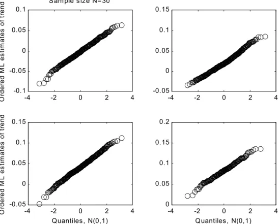
β can reasonably be assumed to follow Normal distributions when estimated from Gumbel-distributed data with sample sizes N = 30 and N=50, quantile plots were calculated, in which linearity indicates conformity with the Normal hypothesis. These plots are shown in Figs. 1 and 2.

This section has described how the properties were obtained of LR and ML estimates of the linear trend parameter β. The non-parametric Mann-Kendall (MK) test for trend, referred to earlier, provides a test for the statistical significance of trend (not necessarily linear) without providing an estimate of the trend magnitude. The following section describes the procedures for comparing the powers of significance tests of the hypothesis H₀: β = 0, against the one-sided alternative H₁: β > 0, and the two-sided alternative H₁: β≠ 0, for the LR, ML and MK approaches.

Method for comparing powers of (a)

ML, (b) LR, (c) MK tests of the

hypothesis ‘trend absent’ (

βββββ

= 0)

against the alternatives

βββββ

> 0 and

βββββ ≠≠≠≠≠

0

The powers of the three tests were compared by simulation. For the ML and LR tests, a 5% critical region was calculated by simulating 600 samples, all from the distribution in (1) for which β = 0. Thus the size of the test was 0.05 in all cases. For each sample generated, the estimated trend coefficients β_MLand βLRwere calculated, together with

either the 95% quantile (where the alternative hypothesis was H₁:β > 0) or the 2.5% and 97.5% quantiles (where the alternative hypothesis was H₁:β≠≠≠≠≠ 0). For the procedures LR1 and ML1, these quantiles then defined regions for which the Type I Error – that is, the error occurring when the null hypothesis H₀:β= 0 is rejected, although true – was known and equal to 5% (that is, in 5% of a very large number of samples from the distribution (1), the estimate_^

β of the linear trend coefficient would fall in the critical region, leading to the conclusion that trend existed where it did not). Having defined the critical regions, sets of 600 samples were again generated for known values of β, now different from zero and given the values shown in Tables (1a); the estimates and were calculated for each sample generated, but this time the proportions (out of 600

samples) falling outside the critical regions were calculated. These proportions estimate the Type II Errors – the probabilities that randomly-selected samples from the distribution (1a), with trend parameter β different from zero, lead to estimates βML, βLRfalling within the region of

acceptance for the null hypothesis H₀: β=0, although that hypothesis is false. Thus, the test size was fixed at 5%, but the Type II Error could be, and was, different for the different test procedures; and the Type II Errors are related to the power of the test through the relation ‘power = 1 – Type II Error’, so that the larger the Type II Error, the smaller is the power of the test. Powerful tests have small Type II Errors, but the magnitude of the Type II Error depends upon the (true but unknown) value of βin the alternative hypothesis H₁.

For the LR2 and ML2 procedures, the critical values for the tests were not determined by simulation, but were determined by the appropriate tabulated values of the t-statistic in the case of LR2, and from the appropriate values of the standard Normal N(0,1) distribution, in the case of ML2, as given in the preceding section. However the Type II Error, and hence the power of each test, was determined by simulating sets of 600 samples, and counting the proportion that fell outside the critical region so determined. For the Mann-Kendall test, the procedure was similar to that used for LR2 and ML2, although the MK test gives no estimate of the trend coefficient. In the MK test, a statistic Z is calculated which, in the absence of trend and for the sample sizes N = 30 and N= 50 used in this paper, has a probability distribution that is well approximated by the standard Normal N(0, 1) distribution. Thus for each of the 600 samples generated with β =0 (the distribution (1)) the test statistic Z was calculated, and the quantiles obtained that defined the 5% critical regions for the test. When the test statistic Z is compared with appropriate deviates from the standard Normal distribution, the 5% critical regions should be |Z| > 1.96 for the two-sided test (H₁: β ≠ 0) and Z > 1.645 for the one-sided test (H₁: β > 0). In fact, the 600 samples from the distribution (1) gave, for the two-sided tests, critical regions –1.76 < Z <1.94 and –1.924 < Z <1.974 for sample sizes N = 30 and N = 50 respectively, and for the one-sided tests, critical regions Z > 1.647 and Z > 1.601 for N = 30 and N = 50. As with the ML and LR test procedures, sets of 600 samples with values of βshown in Table 1(a) were used to establish the proportions out of the 600 samples generated, for which the MK test statistic Z fell outside the critical region, this proportion being an estimate of the Type II Error. Table 2 presents the Type II Errors for N = 30 and N = 50, for one-sided and two-sided alternatives H₁, obtained for the five test procedures.

ML

β βLR

^ ^

^ ^

-4 -2 0 2 4 -0.1

-0.05 0 0.05 0.1

O

rd

e

re

d

M

L

e

s

ti

m

a

te

s

o

f

tr

e

n

d S am ple s ize N= 30

-4 -2 0 2 4

-0.05 0 0.05 0.1 0.15

-4 -2 0 2 4

-0.05 0 0.05 0.1 0.15

Quantiles , N(0,1)

O

rd

e

re

d

M

L

e

s

ti

m

a

te

s

o

f

tr

e

n

d

-4 -2 0 2 4

0 0.05 0.1 0.15 0.2

Quantiles , N(0,1)

Fig. 1.Normal plots of Maximum Likelihood estimates of linear trend parameter β, calculated from 600 samples of size N = 30 drawn from a standard Gumbel distribution (u = 0, a = 1) with superimposed linear trend: trend parameter β = 0, β = 0.02137, β = 0.04275, β= 0.0855.

Table 1(a). Means of 600 samples generated from a standard Gumbel distribution (u =0, a=1) with superimposed trend β of magnitude shown.

N = 30.

Means of estimated trend parameter b (equal to increases in E[Y] of 0, ½σ, σ and 2σ over period of artificial record of length N = 30):

β = 0: β = 0.02137: β = 0.04275: β = 0.0855:

LR: – 0.0003789 + 0.02113 + 0.04276 + 0.08353

(± 0.02_{113) (± 0.0}2_{108) (± 0.0}2_{115) (± 0.0}2₁₀₅₎

ML: – 0.0009326 + 0.02106 + 0.04202 + 0.08368

(± 0.03_{929) (± 0.0}3_{888) (± 0.0}3_{974) (± 0.0}3₈₆₉₎ [Note the convention that 0.03_{869 = 0.000869 or 0.869 × 10}–4_]

N = 50.

Means of estimated trend parameter β(equal to increases in E[Y] of 0, ½σ, σ and 2σ over period of artificial record of length N = 50):

β = 0: β = 0.01282: β = 0.02564: β = 0.0513:

LR: + 0.0002929 + 0.01275 + 0.02583 + 0.05131

(± 0.03_{493) (± 0.0}3_{509) (± 0.0}3_{508) (± 0.0}3₅₂₈₎

ML: + 0.0002303 + 0.01282 + 0.02597 + 0.05125

(± 0.03_{399) (± 0.0}3_{405) (± 0.0}3_{409) (± 0.0}3₄₀₇₎

Table 1(b). Variances of 600 samples generated from a standard Gumbel distribution (u =0, a=1) with superimposed trend βof magnitude shown.

N = 30.

Variances of estimated trend parameter β(equal to increases in E[Y] of 0, ½σ, σ and 2σ over period of artificial record of length N = 30):

β = 0: β = 0.02137: β = 0.04275: β = 0.0855: LR: 0.03_{7624 0.0}3_{6999 0.0}3_{7920 0.0}3₆₆₂₃

ML: 0.03_{5178 0.0}3_{4731 0.0}3_{5692 0.0}3₄₅₂₇

Ratio,

LR/ML: 1.47 1.48 1.39 1.46

N = 50.

Variances of estimated trend parameter β(equal to increases in E[Y] of 0, ½σ, σ and 2σ over period of artificial record of length N = 50):

β = 0: β = 0.01282: β = 0.02564: β = 0.0513:

LR: 0.03_{1459 0.0}3_{1554 0.0}3_{1546 0.0}3₁₆₇₂

ML:0.04_{9547 0.0}4_{9835 0.0}3_{1006 0.0}4₉₉₂₆

Ratio,

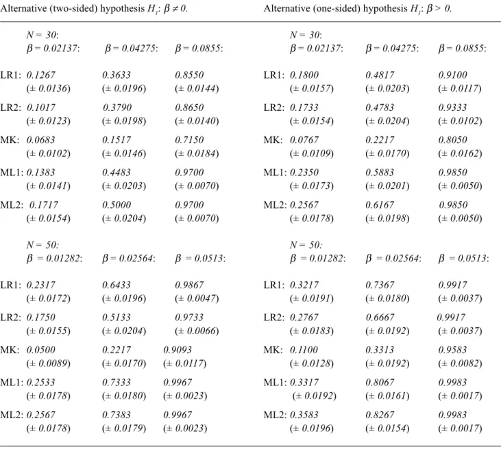
Table 2. Type II Errors for the LR, MK and ML test procedures, all with Type I Error 5%, with one- and two-sided alternatives, and two sample sizes N = 30 and N = 50. Figures in brackets are standard errors.

Alternative (one-sided) hypothesis H₁: β > 0.

N = 30:

β = 0.02137: β = 0.04275: β = 0.0855:

LR1: 0.1800 0.4817 0.9100

(± 0.0157) (± 0.0203) (± 0.0117)

LR2: 0.1733 0.4783 0.9333

(± 0.0154) (± 0.0204) (± 0.0102)

MK: 0.0767 0.2217 0.8050

(± 0.0109) (± 0.0170) (± 0.0162)

ML1:0.2350 0.5883 0.9850

(± 0.0173) (± 0.0201) (± 0.0050)

ML2:0.2567 0.6167 0.9850 (± 0.0178) (± 0.0198) (± 0.0050)

N = 50:

β = 0.01282: β = 0.02564: β = 0.0513:

LR1: 0.3217 0.7367 0.9917

(± 0.0191) (± 0.0180) (± 0.0037)

LR2: 0.2767 0.6667 0.9917 (± 0.0183) (± 0.0192) (± 0.0037)

MK: 0.1100 0.3313 0.9583

(± 0.0128) (± 0.0192) (± 0.0082)

ML1:0.3317 0.8067 0.9983

(± 0.0192) (± 0.0161) (± 0.0017)

ML2:0.3583 0.8267 0.9983

(± 0.0196) (± 0.0154) (± 0.0017) Alternative (two-sided) hypothesis H₁: β≠ 0.

N = 30:

β = 0.02137: β = 0.04275: β = 0.0855:

LR1: 0.1267 0.3633 0.8550

(± 0.0136) (± 0.0196) (± 0.0144)

LR2: 0.1017 0.3790 0.8650 (± 0.0123) (± 0.0198) (± 0.0140)

MK: 0.0683 0.1517 0.7150

(± 0.0102) (± 0.0146) (± 0.0184)

ML1:0.1383 0.4483 0.9700

(± 0.0141) (± 0.0203) (± 0.0070)

ML2: 0.1717 0.5000 0.9700

(± 0.0154) (± 0.0204) (± 0.0070)

N = 50:

β = 0.01282: β= 0.02564: β = 0.0513:

LR1: 0.2317 0.6433 0.9867

(± 0.0172) (± 0.0196) (± 0.0047)

LR2: 0.1750 0.5133 0.9733

(± 0.0155) (± 0.0204) (± 0.0066)

MK: 0.0500 0.2217 0.9093

(± 0.0089) (± 0.0170) (± 0.0117)

ML1:0.2533 0.7333 0.9967

(± 0.0178) (± 0.0180) (± 0.0023)

ML2:0.2567 0.7383 0.9967

(± 0.0178) (± 0.0179) (± 0.0023)

Discussion

Tables 1(a) and 1(b) give the means and variances of estimated values of the single linear trend parameter β estimated by LR and by ML, for the two sample sizes N = 30 and N = 50, obtained by generating 600 artificial samples in each case. Table 1(a) shows that for both sample sizes, the ML estimates are effectively unbiassed (although for N = 30 and β = 0, the mean of the ML estimates of βis well over twice that of the LR estimates that were shown to be unbiassed); for N =30 and positive values of β, the LR and ML means are almost identical. However, Table 1(b) shows marked differences in variances given by the two estimation

procedures; for both sample sizes N = 30 and N= 50, and for all values of the trend parameter β, the variances given by the ML procedure are substantially less than the variances of the LR estimates, although for both sample sizes the ratio var[βLR] / var[βML] is less than its asymptotic value 1.64, being approximately 1.45 for N = 30, and rather larger, about 1.58, for N = 50. This suggests that, when the record length N is smaller than that for which asymptotic results can be expected to apply, there is still a substantial gain in the precision with which the trend parameter β is estimated by ML, relative to the precision given by LR, but the reduction in variance is proportionately smaller.

A point of interest concerns the variances of βLRand of ML

β when the true trend is zero, β = 0. It was shown above that var[β_LR] = π2 _{/( 6a}2 _S

tt) = 2π

2_/[N(N2_{-1)] =}

0.03_{73189 and 0.0}3_{15798 for N = 30 and N = 50 respectively,}

when the t-values are equally spaced; the variances of βLR

obtainedfor the two sets of 600 simulated samples are close to these values, 0.03_{7624 and 0.0}3_{1459 respectively.}

Similarly for var[βML] = 12 / [a

2_N(N2 _{– 1) ]; for N = 30, N}

= 50 and α =1, this has values 0.03_{4449 and 0.0}4_96038,

and the variances of βMLobtained in the simulations were

0.03_{5178 and 0.0}4_{9547 respectively.}

With regard to the Normality of the ML estimates of β, Figs. 1 and 2 show no evidence that it would be inappropriate to assume that βML is Normally distributed, even for

samples as small as N = 30.

Table 2, giving the Type II Errors for the LR, MK and ML test procedures, shows that these errors are greatest for the Mann-Kendall test, the difference between this and LR, ML being especially marked as the trend coefficient β increases. As expected, the Type II Errors are smaller for N = 50 than for N = 30, more ‘data’ providing better sensitivity; while for all three tests, the errors diminish with increasing β, as expected. For all values of β and both sample sizes, ML estimation has smaller Type II Errors than either MK or LR test procedures, the difference between ML and LR is not very great when β is small, but is very substantial for larger values of β.

Conclusion

The case has been discussed where sequences of hydrological data can be expected to follow a Gumbel distribution, possibly with time-variant mean. It has been assumed that the time-trend in mean value is determined by a single parameter β to be estimated by Maximum Likelihood (ML). The large-sample variance of the ML estimate βML has been compared with the variance of the

trend βLR calculated by linear regression; the latter was

found to be 64% greater. Simulated samples from a standard Gumbel distribution were given superimposed linear trend of different magnitudes, and the power of three procedures for testing the existence of linear trend (Maximum Likelihood, Linear Regression and the non-parametric Mann-Kendall test) were compared. ML procedures were always the most powerful; the MK test procedure was always the least powerful by a substantial margin.

References

Bruijnzeel. L.A., 1996. Predicting the hydrological impacts of land cover transformation in the humid tropics: the need for integrated research. In: Amazonian Deforestation and Climate, J.H.C. Gash, C.A. Nobre, J.M. Roberts and R.L. Victoria, (Eds.). Wiley, Chichester, UK. 15–55.

Bruijnzeel, L.A., 1990. Hydrology of Moist Tropical Forests and

Effects of Conversion: A State of Knowledge Review, IHP/IAHS/

UNESCO, Paris. 224pp.

Clarke, R.T., 2002a. Estimating Time Trends in Gumbel-Distributed Data by Means of Generalized Linear Models. Water

Resour. Res. (in press).

Clarke, R.T., 2002b. Estimating trends in data from the Weibull and a GEV distribution. Water Resour. Res., (in press) Changnon, S.A. and Kunkel, K.E., 1995. Climate-related

fluctuations in Midwestern floods during 1921-1985. J. Water

Resour. Plan. Man, 121, 326–334.

Douglas, E.M., Vogel, R.M. and Kroll, C.N., 2000. Trends in floods and low flows in the United States: impact of spatial correlation. J. Hydrol., 240, 90–105.

Green, P.J., 1984. Iteratively reweighted least squares for maximum likelihood estimation, and some robust and resistant alternatives (with discussion). J. Roy. Stat. Soc B, 46, 149–92. Groisman, P.Y. and Easterling, D.R., 1994. Variability and trends in total precipitation and snowfall over the United States and Canada. J. Climatol., 7, 184–205.

Guttman, N.B., Wallis, J.R. and Hosking, J.R.M., 1992. Regional temporal trends of precipitation quantiles in the US. Research

report RC 18453 (80774), IBM Research Division, Yorktown

Heights, NY.

Hirsch, R.M., Helsel, D.R., Cohn, T.A. and Gilroy, E.J., 1993. Statistical Analysis of Hydrologic Data. In: Handbook of

Hydrology, D.R. Maidment (Ed.), McGraw-Hill, New York.

17.1–17.55.

IPCC Report, Climate Change 2001: Report of Working Group II

Impact, Adaptation and Vulnerability, http://www.ipcc.ch.

McCullagh, P. and Nelder, J.A., 1983. Generalised Linear Models

(2nd _{edition), Chapman and Hall, London.}

Olsen, J.R., Stedinger, J.R, Matalas, N.C. and Stakhiv, E.Z., 1999. Climate variability and flood frequency estimation for the upper Mississippi and lower Missouri rivers. J. Amer. Water Resour.

Assoc., 35, 1509–1520.

Natural Environment Research Council, 1975. NERC Flood

Studies Report, Volume 1.

Salas, J.D., 1993. Analysis and Modeling of Hydrologic Time Series. In: Handbook of Hydrology, D.R. Maidment (Ed.), McGraw-Hill, New York. 19.1–19.72.

Sahin, V. and Hall, M.J., 1996. The effects of afforestation and deforestation on water yields. J. Hydrol.,178, 293–309. Stedinger, J.R., Vogel, R.M. and Foufoula-Georgiou, E., 1993.

Frequency Analysis of Extreme Events. In: Handbook of

Hydrology, D.R. Maidment (Ed.), McGraw-Hill, New York.

18.1–18.66.

Vinnikov, K.Y., Groisman, P.Y. and Lugina, K.M., 1990. Empirical data on contemporary global climate change (temperature and precipitation). J. Climatol., 3, 662–677.

^

^

^

^

^

^

^