Return distribution and value at risk estimation for BELEX15

DOI: 10.2298/YJOR1101103D

RETURN DISTRIBUTION AND VALUE AT RISK

ESTIMATION FOR BELEX15

Dragan

Đ

ORI

Ć

Faculty of Organizational Sciences, University of Belgrade, [email protected]

Emilija NIKOLI

Ć

-

Đ

ORI

Ć

[email protected]

Received: October 2010 / Accepted: February 2011

Abstract: The aim of this paper is to find distributions that adequately describe returns of the Belgrade Stock Exchange index BELEX15. The sample period covers 1067 trading days from 4 October 2005 to 25 December 2009. The obtained models were considered in estimating Value at Risk (VaR) at various confidence levels. Evaluation of VaR model accuracy was based on Kupiec likelihood ratio test.

Keywords: Value at risk, return distributions, Kupiec test, BELEX15.

MSC: 91B30, 62E99, 60G70.

1. INTRODUCTION

Value at Risk (VaR) is a commonly used statistic for measuring potential risk of economic losses in financial markets [11, 5, 4, 8]. Using VaR financial institutions can calculate the possible maximum loss over a given time horizon, usually 1-day or 10 days, at a given confidence level. Empirical VaR calculations involve the estimation of lower-order quantiles, for example 10%, 5% or 1% of the return distribution. While VaR concept is very easy, its measurement is a very challenging statistical problem. Risk analysis can be done in two stages. First, we can express profit-and-loss in terms of returns, and subsequently, model the returns statistically and estimate theVaR of returns by computing appropriate quantile.

approximation of the true distribution of returns which is reasonably accurate in the center of the distribution. However, to estimate an extreme quantile such as VaR, we need a reasonable estimate not just in the centre of the distribution but in the extreme tail as well. Standard VaR measure presumes that asset returns are normally distributed, whereas it is widely documented that they really exhibit non-zero skewness and excess kurtosis and, hence, the VaR measure either underestimates or overestimates the true risk [1]. It is well known that the probability distribution of stock returns is fat tailed, which means that extreme price movements occur much more often than predicted given a Gaussian model [7].

Besides the heavy-tailed issue, asymmetry distribution is also often observed in financial time series. This property is very important in risk analysis where the long and short position investments over a given time period relied heavily on the lower and upper tails behaviours. Barndorff-Nielsen [2] implemented skewed distributions that allowed upper and lower tails to have dissimilar behaviours.

In recent years there has been a lot of research conducted on VaR estimation of different returns series [8, 14, 10], but research papers dealing with VaR calculation in the financial markets of EU new member states are very rare. Živkovic [16] applied VaR methodology and historical simulation on the Croatian stock market indices in an effort to measure Value-at-Risk. He also [15] analysed VaR models for ten national indexes: Slovenia - SBI20, Poland - WIG20, Czech Republic - PX50, Slovakia - SKSM, Hungary - BUX, Estonia - TALSE, Lithuania - VILSE, Latvia - RIGSE, Cyprus - CYSMGENL, Malta - MALTEX and concluded that use of common VaR models to forecast VaR is not suitable for transition economies.

In this paper the relative performance of VaR models of Belgrade Stock Exchange index BELEX15 was investigated. The rest of the paper is organized as follows. Section 2 describes the basic concept of VaR and presents various static models for VaR. Evaluating VaR model adequacy is given in Section 3. Section 4 presents empirical results obtained by applying described models to stock index BELEX15. While most empirical studies focused only on holding a long position, we also consider a short position. Concluding remarks are given in Section 5.

2. STATIC VAR MODELS

Let Pt be the price of a financial asset on day t. A k-day VaR of a long position

on day t is defined by

( t t k ( , , )) ,

P P−P− ≤VaR t kα =α (1)

where (0, 0.5)α ∈ . Similary, a k day VaR of a short position is defined by

. )) , , (

(P −P₋ ≥VaR t k α =α

P _{t t k} (2)

of a percentile of the return distribution [4]. If qα is the α th percentile of the return, then VaR of a long position can be written as

k t q

P e k t

VaR(, ,α)=( α −1) − (3)

From (3) it can be seen that good VaR estimates can be produced with accurate forecasts of the percentiles q_α. So, in further we consider only VaR for return series.

We define the 1-day logarithmic return (in further text just return) on day t as

1

log( ) log( )

t t t

r = P − P− (4)

and denote the information up to time t by Ft. That is, for a time series of returns rt,

VaR is such that

1

(t t t )

P r <VaR F− =α (5)

From this, it is clear that finding a VaR essentially is the same as finding a 100α % conditional quantile. For convention, the sign is changed to avoid negative number in the

VaR.

Unconditional parametric models assume that the returns are iid (independent identically distributed) with density given by

1

( ) ( ),

r r

x

f x f μ

σ ∗ σ

−

= (6)

with fr being density function of the distribution of rt and fr∗ being density function of

the standardized distribution of rt. The parameters μ and σ are mean value and

standard deviation of rt.

The static VaR for return rt for long trading positions is given by

*

long

VaR = +μ r_ασ (7)

and for short trading positions it is equal to

* 1

short

VaR = +μ r−_ασ (8)

Where rα* isα quantile of fr*.

This section will briefly introduce the models of asset return distributions that are to be investigated and compared with one another. These include normal, Student t, NIG (Normal Inverse Gaussian), hyperbolic and stable distributions.

Fitting returns with Normal distribution

, 2 ) ( exp 2 1 ) ( 2 2 ⎪⎭ ⎪ ⎬ ⎫ ⎪⎩ ⎪ ⎨ ⎧ − − = σ μ σ π x x

f (9)

where μ is the mean, and σ is the stardard deviation. We fit a normal distribution using the Maximum Likelihood (ML) estimates for the mean μ and the standard deviation (σ )

1/ 2 2

1 1

1 1

ˆ , ˆ ( ˆ) ,

n n

i i

i i

r r

n n

μ σ μ

= =

⎛ ⎞

= =_⎜ − _⎟

⎝ ⎠

∑

∑

where n is the number of observations in the return series.

Fitting returns with Student t_distribution

Student t distribution has become a standard benchmark in developing models for asset return distribution because it is able to describe fat tails observed in many empirical distributions. Also, its mathematical properties are well known. The density function of a scaled Student t-distribution with zero expectation is given by

( 1) / 2 2

( / 2 1/ 2)

( ) 1 ,

( / 2

x f x b b ν ν ν ν πν − + ⎛ ⎞ Γ + = ⋅ +_{⎜ ⎟}

Γ ⎝ ⎠ (11)

where 2ν > (degrees of freedom) and b>0 (scale parameter). For ν >2 we have

( ) 2 b

VaR X ν

ν =

− . When ν =1 the Student density function is the Cauchy density

function and when ν → ∞ the Student distribution converges to the normal distribution. Taking x= −rt μˆ we fit t distribution to the mean adjusted return series and obtain the

ML estimates, ˆν and ˆb.

Fitting returns with NIG distribution

The Normal Inverse Gaussian (NIG) distribution is characterized by four parametersα ,β ,δ and μ. Its density function is given by

2 2 2 2 ( ) 1 2 2 ( ( ) ) ( ) ( ) x NIG K x

f x e

x

δ α β β μ

α δ μ

αδ

π _{δ μ}

− + −

+ −

= ⋅ ⋅

+ − (12)

where K1 denotes the modified Bessel function of the third kind of order 1. The

means heavier right tail. The value β =0 implies the symmetric distribution around mean. The parameters σ and μ correspond to the scale and location of the distribution.

Fitting returns with hyperbolic distribution

The hyperbolic distribution had been used in various fields before it was applied to finance by Eberlein and Keller [6]. The hyperbolic distribution permits heavier tails than the normal distribution because its log-density is a hyperbola, instead of a parabola in case of normal distribution. Its density function is defined by

2 2 2 2 ( ) ( ) 2 2 1 ( ) ,

2 ( )

x x H

f x e

K

α δ μ β μ

α β

αδ δ α β

− + − + −

−

= ⋅

− (13)

where α ,β ,δ and μ are parameters and K1 is the modified Bessel function of the

third kind with index 1. Parameters α and β determine the shape of the density while

δ and μ determine the scale and location.

There are also other parametrizations for the density function, for example

2 2 2 2

( ( ) ( )) ( ( ) ( ))

2 2

1

( )

( ) ( )

x x x x

H

f x e

K

ϕ _{δ μ μ} γ _{δ μ μ}

ϕγ

δ ϕ γ δ ϕγ

− + − − − − + − + −

= ⋅

+ (14)

with ϕ α β= + and γ α β= − .

Fitting returns with stable distribution

Mandelbrot [13] and Fama [7] first proposed the stable distribution to model stock returns. Although most stable distributions and their probability densities cannot be described in closed mathematical form, their characteristic functions can be expressed in closed form. Stable distributions are characterized by four parameters α ,β ,δ and μ and the characteristic function of the general stable distribution is given by

⎪ ⎪ ⎩ ⎪ ⎪ ⎨ ⎧ = ⎭ ⎬ ⎫ ⎩ ⎨ ⎧_{− + ⋅ ⋅ +} ≠ ⎭ ⎬ ⎫ ⎩ ⎨ ⎧_{− − ⋅ +} = 1 )) ( ln 2 1 ( exp 1 )) ( 2 tan 1 ( exp ) ( α μθ θ θ π β θ σ α μθ θ πα β θ

σα α

θ i sign i i sign i e

E i X (15)

The characteristic exponent or index α lies in the half-open interval (0,2] and measures the rate at which the tails of the density function decline to zero. The skewness parameter

β lies in the closed interval [-1,1] and is a measure of the asymmetry of the distribution. The stable distribution can be skewed to the left or right, depending of the sign of β . The scale parameter σ >0 measures the spread of the distribution and the location parameter μ is a rough measure of the midpoint of the distribution. The stable

A stable distribution with characteristic exponent α has moments of order less than α and does not have moments of order greater than α . If α =0 and β =0, the stable distribution is the Cauchy distribution. If α =2 and β =0, the stable distribution is the normal distribution. If 1< <α 2, the most plausible case for financial series, the tails of stable distribution are fatter than those of the normal and the variance is infinite. Stable distributions as a class have the attractive feature that the distribution of sums of random variables from a stable distribution retains the same shape and skewness, although resulting distribution will change its scale and location parameters. Furthermore, they are the only class of statistical distributions having this feature.

If the returns are assumed to follow a stable distribution, the procedure for calculating VaRs remains unchanged. The quantile has to be derived from the standardized stable distribution S_α( ,1, 0)β .

3. EVALUATING VAR MODEL ADEQUACY

Various methods and tests have been suggested for evaluating VaR model accuracy. Performance of the VaRs for different pre-specified level α can be evaluated by computing their failure rate for the returns. Statistical adequacy could be tested based on Kupiec likelihood ratio test which examines whether the average number of violations is statistically equal to the expected rate.

3.1 Failure rate

The failure rate is widely applied in studying the effectiveness of VaR models. The definition of failure rate is the proportion of the number of times the observations exceed the forecasted VaR to the number of all observations. If the failure rate is very close to the pre-specified VaR level, it could be concluded that the VaR model is specified very well.

3.2 Kupiec likelihood ratio test

For the purpose of testing VaR models in a more precise way, the Kupiec LR test for testing the effectiveness of our VaR models is adopted. A likelihood ratio test developed by Kupiec [12] will be used to find out whether a VaR model is to be rejected or not. The number n of VaR violations in a sample of size T has a binomial distribution, n~ ( , )B T p . The failure rate is /n T and, ideally, it should be equal to the left tail probability, p. The null H0 and alternative H1 hypotheses are:

0: , 1:

n n

H p H p

T = T ≠ (16)

where

1

(t p t )

p=P r <VaR F− (17)

2 log( n(1 )T n) log( n(1 )T n)

LR= ⎡_⎣ q −q − − p −p − ⎤_⎦ (18)

where /q=n T. This likelihood ratio is asymptotically χ₁2 distributed under the null hypothesis that p is the true probability the VaR is exceeded. With a certain confidence level we can construct nonrejection regions that indicate whether a model is to be rejected or not. Therefore, the risk model is rejected if it generates too many or too few violations.

However, Kupiec test can accept a model which incurs violation clustering but in which the overall number of violations is close to the desired coverage level. For other ways of testing VaR models see [3].

4. EMPIRICAL RESULTS

4.1 Data

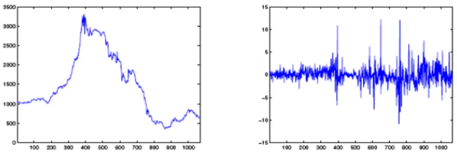
The data used in the paper are the market index BELEX15 of the Belgrade Stock Exchange and they are obtained from the BELEX website. BELEX15, leading index of the Belgrade Stock Exchange, describes the movement of prices of the most liquid Serbian shares (includes shares of 15 companies) and is calculated in real time. The sample period covers 1067 trading days from 4 October 2005 to 25 December 2009. The plots of the BELEX15 index and returns are given in Figure 1. In this section, the return r_tis expressed in percentages, i.e. r_t =100(logP_t−logP_t−1).

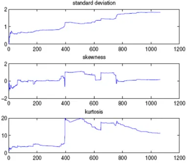
Figure 2: Standard deviation, skewness and kurtosis for BELEX15 up to a point

Results of Augmented Dickey-Fuller test with exogenous constant, linear trend and autocorrelated terms of order selected by Schwarz information criterion, applied on series of daily index, confirm the presence of a unit root (ADF= −1,1461,p=0.9194). Null hypothesis of presence of unit roots for returns is rejected

(ADF = −22.0975,p=0.0000). Visual inspection of returns shows that the variances change over time around some level, with large (small) changes tending to be followed by large (small) changes of either sign (volatility tends to cluster). Periods of high volatility can be distinguished from low volatility periods. In order to check if moments of order two to four are finite, samples up to date are used to calculate standard deviation, skewness and kurtosis (Figure 2). It is evident that after approximately 800 observations these sample moments became stable, which supports conclusion about finiteness of corresponding population values.

Descriptive statistics

Table 1: Descriptive Statistics of BELEX 15 index returns

mean median min max variance skewness kurtosis

BELEX 15 -0.0433 -0.0326 -10.8614 12.15676 3.3144 0.1752 11.3420

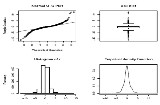
Figure 3: Empirical distribution for BELEX15 returns

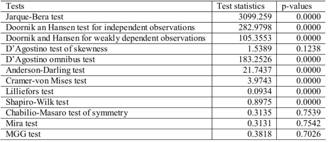
Table 2: Statistical tests for distribution of returns

Tests Test statistics p-values

Jarque-Bera test 3099.259 0.0000

Doornik an Hansen test for independent observations 282.9798 0.0000 Doornik and Hansen for weakly dependent observations 105.3553 0.0000

D’Agostino test of skewness 1.5389 0.1238

D’Agostino omnibus test 183.2526 0.0000

Anderson-Darling test 21.7437 0.0000

Cramer-von Mises test 3.9743 0.0000

Lilliefors test 0.0934 0.0000

Shapiro-Wilk test 0.8975 0.0000

Chabilio-Masaro test of symmetry 0.3135 0.7539

Mira test 0.3131 0.7542

MGG test 0.3818 0.7026

4.2 Static VaR models

Static models include historical simulation and fitting several distributions to empirical returns. Six common values of α were chosen for illustration. They are 10%, 5%, 2%, 1% 0.5% and 0.1%.

Historical Simulation

Historical Simulation of VaR is based on quantile estimates of return distribution quantiles. The sample quantiles can be obtained by several different algorithms [9]. Here is an applied algorithm recommended by the same authors. VaR values for all chosen α for both a long and a short position are given in the Figure 4 and the Table 3.

Table 3: BELEX15 - VaR by nonparametric Historical Simulation Historical simulation

α 10% 5% 2% 1% 0.5% 0.1%

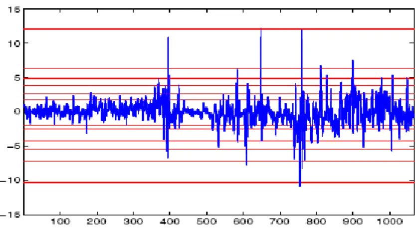
Figure 4: Daily returns and VaR by nonparametric Historical Simulation

Fitting Distributions

Parametric approach for calculating VaR is based on modelling empirical return distribution with some theoretical distribution. Then VaR is the corresponding quantile of theoretical distribution. In this analysis normal, Student, NIG, hyperbolic and stable distributions were applied. Distribution parameters were estimated using Matlab MFE Toolbox [17].

Table 4: BELEX15 - Parameter estimates of the theoretical distributions

μ σ ν α β δ

Normal -0.0433 1.8197 - - - -

Student -0.0433 0.01105 3 - - -

NIG -0.0646 1.1074 - 0.3271 0.0064 -

Hyperbolic -0.0826 0.0621 - 0.8251 0.0134 -

Figure 5: Empirical and theoretical CDF’s and left distribution tails of BELEX15 daily returns

Parameters of the distribution fitted to the data are presented in Table 4. Empirical and theoretical cumulative density functions are presented in Figure 5. It can be seen that CDF’s of theoretical distributions are much closer to each other than corresponding tails of distributions. For both tails NIG distribution is the closest to empirical data as seen in Figure 5.

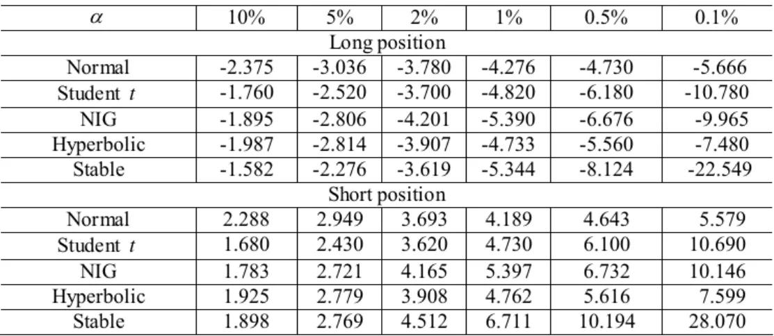
Table 5: VaR values of BELEX15 returns based on theoretical distributions

α 10% 5% 2% 1% 0.5% 0.1%

Long position

Normal -2.375 -3.036 -3.780 -4.276 -4.730 -5.666 Student t -1.760 -2.520 -3.700 -4.820 -6.180 -10.780

NIG -1.895 -2.806 -4.201 -5.390 -6.676 -9.965

Hyperbolic -1.987 -2.814 -3.907 -4.733 -5.560 -7.480 Stable -1.582 -2.276 -3.619 -5.344 -8.124 -22.549

Short position

Normal 2.288 2.949 3.693 4.189 4.643 5.579

Student t 1.680 2.430 3.620 4.730 6.100 10.690

NIG 1.783 2.721 4.165 5.397 6.732 10.146

Hyperbolic 1.925 2.779 3.908 4.762 5.616 7.599

Stable 1.898 2.769 4.512 6.711 10.194 28.070

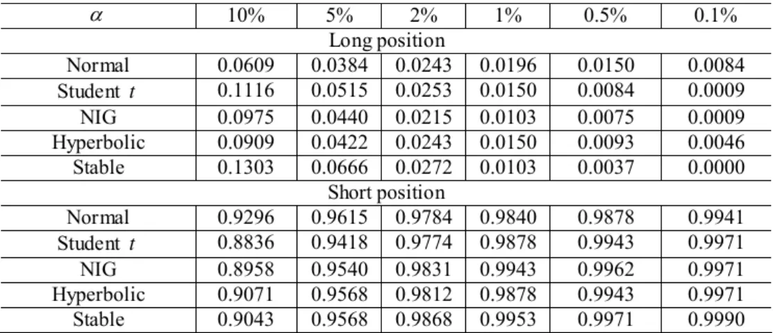
Table 6: VaR failure rates of BELEX15 returns based on theoretical distributions

α 10% 5% 2% 1% 0.5% 0.1%

Long position

Normal 0.0609 0.0384 0.0243 0.0196 0.0150 0.0084 Student t 0.1116 0.0515 0.0253 0.0150 0.0084 0.0009

NIG 0.0975 0.0440 0.0215 0.0103 0.0075 0.0009

Hyperbolic 0.0909 0.0422 0.0243 0.0150 0.0093 0.0046 Stable 0.1303 0.0666 0.0272 0.0103 0.0037 0.0000

Short position

Normal 0.9296 0.9615 0.9784 0.9840 0.9878 0.9941 Student t 0.8836 0.9418 0.9774 0.9878 0.9943 0.9971

NIG 0.8958 0.9540 0.9831 0.9943 0.9962 0.9971

Hyperbolic 0.9071 0.9568 0.9812 0.9878 0.9943 0.9971 Stable 0.9043 0.9568 0.9868 0.9953 0.9971 0.9990

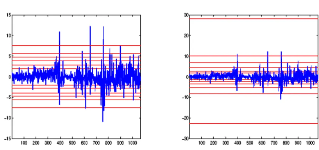
Figure 6: VaR - Normal (on the left), NIG (on the right)

Figure 7: VaR - Hyperbolic (on the left), stable (on the right)

Table 7: Violations of VaR values for theoretical distributions

α 10% 5% 2% 1% 0.5% 0.1%

Long position

Expected 107 53 21 11 5 1

Normal 65 41 26 21 16 9

Student t 119 55 27 16 9 1

NIG 104 47 23 11 8 1

Hyperbolic 97 45 26 16 10 5

Stable 139 71 29 11 4 0

Short position

Expected 959 1013 1045 1055 1061 1065

Normal 991 1025 102 1049 1053 1060

Student t 942 1004 1004 1053 1060 1063

NIG 955 1017 1017 1060 1062 1063

Hyperbolic 967 1020 1020 1053 1060 1063

Stable 964 1020 1020 1061 1063 1065

From the Figure 6 and Figure 7 we can see VaR values for different α and for Normal, NIG, hyperbolic and stable distributions. It is obvious that normal distribution underestimates while stable distribution overestimates VaR values.

Table 7 contains the number of VaR value violations for different distributions together with expected values. The conclusion is that none of the considered distributions are superior for all α . For long position and α =0.1 and α =0.2 NIG is better than other considered distributions. For α =0.01 violations of VaR for NIG and Student t are equal to expected values and for α =0.001 the same conclusion is valid for NIG and stable distributions. In the case of short position NIG is superior for α =0.01and

0.05

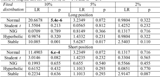
Table 8: Kupiec test for α = 10%, α = 5% and α = 2%

10% 5% 2% Fited

distribution LR p LR p LR p

Long position

Normal 20.6678 5.4e-6 3.2349 0.072 0.9804 0.322

Student t 1.5504 0.213 0.0565 0.812 1.4252 0.232

NIG 0.0709 0.789 0.8149 0.366 0.1317 0.716

Hyperbolic 0.9874 0.320 1.4332 0.231 0.9804 0.322

Stable 10.085 0.001 5.6287 0.017 2.5403 0.110 Short position

Normal 11.4903 6.e-4 3.2349 0.072 0.1317 0.716

Student t 3.0146 0.082 1.4235 0.232 0.3304 0.565

NIG 0.1993 0.655 0.655 0.540 0.5566 0.455

Hyperbolic 0.6152 0.432 1.1013 0.293 0.0851 0.770

Stable 0.2234 0.636 1.1013 0.293 2.9147 0.087

Table 9: Kupiec test for α = 1%, α = 0.5% and α = 0.1%

1% 0.5% 0.1% Fited

distribution LR p LR p LR p

Long position

Normal 7.8986 0.0004 13.9433 1.8e-4 22.5909 2.e-6

Student t 2.3419 0.125 2.1024 0.147 0.0041 0.948

NIG 0.0108 0.917 1.1641 0.280 0.0041 0.948 Hyperbolic 2.3419 0.125 3.2652 0.070 7.6018 0.005

Stable 0.0108 0.917 0.3652 0.545 2.1330 0.144 Short position

Normal 3.2264 0.072 7.798 0.004 10.889 9.6e-4

Student t 0.4849 0.486 0.0813 0.775 2.3437 0.125

NIG 2.4436 0.117 0.3652 0.545 2.3437 0.125

Hyperbolic 0.4849 0.486 0.0813 0.775 0.3140 0.575

Stable 3.7797 0.051 1.2166 0.270 0.7510 0.386

5. CONCLUDING REMARKS

The purpose of this paper has been to consider several alternative models of return distribution for BELEX15 and to compare predictive ability of VaR estimates based on them. First, the data are analysed in order to get an idea of the stylized facts of stock market returns. Throughout the analysis, a holding period of one day was used. Various values for the left tail probability level were considered, ranging from the very conservative level of 0.01 percent to the less cautious 10 percent.

although it is typical for many stock indexes. Since distribution of log-returns exhibits leptokurtosis, several models of leptokurtic distribution were chosen: Student t, NIG, hyperbolic and stable. For both tails NIG distribution is the closest to empirical data. Also, estimated NIG distribution has finite moment of fourth order, which is in accordance with empirical up to a point analysis given in Figure 2. However, based on evaluation of VaR, Student t and NIG distribution are acceptable for all considered α -values. Although static models can not reproduce volatility clustering, they may be successful in modelling tails of distribution and computing VaR of the Belgrade Stock Exchange index BELEX15.

Acknowledgement

The second author is supported in part by the Ministry of Education and Science of the Republic of Serbia(grant no. 43007).

REFERENCES

[1] Alexander, C., Market Models - A Guide to Financial Data Analysis, John Wiley & Sons, New York, 2001.

[2] Barndorff-Nielsen, O.E., “Normal inverse Gaussian distributions and the modelling of stock returns”, Scandinavian Journal of Statistics, 24 (1997) 1-13.

[3] Christoffersen, P., “Evaluating interval forecasts”, International Economic Review, 39 (1998) 841-862.

[4] Dowd, K., Measuring Market Risk, John Wiley & Sons Ltd., New York, 2002.

[5] Duffie, D., and Pan, J., An overview of value at risk”, The Journal of Derivatives, 5 (1997) 749.

[6] Eberlein, E., and Keller, U., “Hyperbolic distributions in finance”, Bernoulli 1 (1995) 281-299.

[7] Fama, E., “The behaviour of stock prices”, Journal of Bussines, 47 (1965) 244-280.

[8] Giot, P., and Laurent, S., “Value-at-risk for long and short trading positions”, Journal of Applied Econometrics, 18 (2003) 641-664.

[9] Hyndman, R. J., and Fan, Y., “Sample quantiles in statistical packages”, American Statistician, 50 (1996) 361-365.

[10] Huang, Y.C., and Lin, B-J., “Value-at-risk analysis for taiwan stock index futures: fat tails and conditional asymmetries in return innovations”, Review of Quantitative Finance and Accounting, 22 (2004) 79-95.

[11] Jorion, P., Value at Risk: The New Benchmark for Controlling Market Risk, McGraw- Hill. [12] Kupiec, “Techniques for verifying the accuracy of risk measurement models”, Journal of

Derivatives, 2 (1995) 73–84.

[13] Mandelbrot, B., “The variations of certain speculative prices”, Journal of Business, 36 (1963) 394-419.

[14] Sarma, M., Thomas, S., and Shah, A., “Selection of VaR models”, Journal of Forecasting, 22 (4) (2003) 337-358.

[15] Živković, S., “Measuring market risk in EU new member states”, Dubrovnik Economic Conference, Dubrovnik, Croatia, 2007.

[16] Živković, S., “Testing popular VaR models in EU new member and candidate states”, Zbornik radova, Ekonomski fakultet, Rijeka, 25 (2) (2007) 325-346.