J. Braz. Soc. Mech. Sci. & Eng. vol.34 número especial 2

M. Suptille

mickael.suptille@insa-rouen.fr

E. Pagnacco

Emmanuel.Pagnacco@insa-rouen.fr

L. Khalij

Leila.Khalij@insa-rouen.fr

J. E. Souza de Cursi

J. Brossard

Generation of Stationary Gaussian

Processes and Extreme Value

Distributions for High-Cycle Fatigue

Models – Application to Tidal Stream

Turbines

The operating environment of tidal stream turbines is random due to the variability of the sea flow (turbulence, wake, tide, streams, among others). This yields complex time-varying random loadings, making it necessary to deal with high cycle multiaxial fatigue when designing such structures. It is thus required to apprehend extreme value distributions of stress states, assuming they are stationary multivariate Gaussian processes. This work focus on such distributions, addressing their numerical simulation with an analytical description. For that, we first focused on generating one-dimensional Gaussian processes, considering a band-limited white noise in both the narrow-band and the wide-band cases. We then fitted the resulting extreme value distributions with GEV distributions. We secondly extended the generation method to the correlated two-dimensional case, in which the joint extreme value distribution can be obtained from the associated margins. Finally, an example of application related to tidal stream turbines introduces a Bretschneider spectrum, whose shape is commonly encountered in the field of hydrology. Comparing the empirical calculations with the GEV fits for the extreme value distributions shows a very well agreement between the results.

Keywords: stochastic processes generation, correlated Gaussian processes, multivariate extreme value distribution, high cycle fatigue, tidal stream turbines

Introduction

Nowadays, it has become necessary to make the most of renewable energies. Tidal stream turbines allow this by harnessing the kinetic energy of sea streams (see Fig.??). But in order to come through they have to be economically competitive, which implies reduced maintenance. However, they are immersed in flows having not mastered characteristics resulting from many contributions such as turbulence, wake, swell, current, etc. These structures are then submitted to random time-varying multiaxial stress states, which can be described from probability distributions associated to a time evolution. Numerically, these stress states can be estimated from a statistical description of the sea load that acts on these submerged structures; see for example Theodorsen (1934), Gmür (1997), Guéna et al. (2006) and Thresher et al. (2009). Such stresses imply a risk of fatigue failure which must be taken into account during the design stage to ensure structural integrity. In this study, we are concerned with the infinite fatigue life, that is based on the greatest stress values reached during the service life (Lambert et al., 2010; Khalij et al., 2010). By taking into account their randomness, this leads us to study their multivariate extreme value distributions. We assume that the stress states are stationary multivariate Gaussian processes, described by their means and power spectral densities. More specifically, we focus in this paper on the way to get, from numerical simulations, bivariate extreme value distributions of components of the stress tensor, with analytical descriptions of the results. Since the mechanical stresses reach their maximum value on the skin of the structure, we shall consider the plane stress case only.

The paper is divided in three parts. The first part deals with generating one-dimensional Gaussian processes in order to evaluate its empirical extreme value distribution. Then, we perform a fit with a GEV distribution. Secondly, these concepts are adapted to

multi-dimensional Gaussian processes and applied to a bivariate correlated case. A bivariate extreme value distribution, evaluated from the associated margins, is found to be a well-adapted model. Finally, we apply the previous considerations to a realistic example related to tidal stream turbines.

Figure 1: Projects of tidal stream turbines: Skerries Islands, Wales, 2015 (left) and Islay strait, Scotland, 2015 (right).

Nomenclature

Acronyms

AR = Average Random

EV D = Extreme Value Distribution

GEV = Generalized Extreme Value

IFFT = Inverse Fast Fourier Transform

MA = Moving Average

PSD = Power Spectrum Density

Operators

arg[•] = argument of the complex number• E[•] = statistical expectation of• Prob[•] = probability of the event_•

Re[•] = real part of•

V[•] = statistical variance of_•

|•| = modulus of the complex number• h•i = temporal mean of•

Latin Symbols

f = frequency (Hz)

j = imaginary unit

m = association parameter between the maxima of two processes

mi =i-th spectral moment

n = number of stochastic processes

nf = number of frequencies

sp = thresholds associated to the maximum of thep-th process (MPa)

t = time (s)

F = cumulative distribution function

Fpq = bivariate distribution function between the p-th and the q-th processes

Fp = marginal distribution function of thep-th process N0 = number of cycles

R = auto-correlation function (MPa²)

Rpz = component of correlation function matrixR(MPa²) S = PSD of a single process (MPa²/Hz)

S = PSD matrix (MPa²/Hz)

Sxx = traction component of the stress tensor (MPa) Sxy = shear component of the stress tensor (MPa) T = samples duration (s)

X = stochastic process (MPa)

Calligraphic Symbols

U _{= uniform distribution} R = Rayleigh distribution

N = normal distribution Greek Symbols

µXp = statistical mean of the process Xp(MPa)

µ_X(r)

p = temporal mean of ther-th realization of the process Xp (MPa)

ρ = auto-correlation coefficient

ρm = correlation coefficient between the maxima of two processes

σ = standard deviation (MPa) ω = angular frequency (rad/s)

The One-Dimensional Case

Let us consider a stationary process characterized by its one-sided PSD, measured in MPa²/Hz and denoted by S, and its statistical distribution: both these quantities provide the frequency distribution of the process. Classically, two extreme situations may be considered: wide-band and narrow-band cases. Let us introduce the frequency f, measured in Hz. Both the cases may be illustrated by considering a band-limited white noise:

S(f) =

(

S0 iff∈(f1,f2]

0 else . (1)

For instance:

• the narrow-band case corresponds to|f2−f1|“small”: in the sequel, we take f1=9.5 Hz, f2=10.5 Hz,S0=7 MPa2/Hz, the frequency f1 being included in the spectral definition domain;

• the wide-band case corresponds to |f2−f1|“large”: in the sequel, we take f1=0 Hz, f2=20 Hz,S0=0.35 MPa2/Hz, the frequency f1 being excluded from the spectral definition domain, since it is the zero value.

It should be noted that in either case,S0is such that V[X(t)] =7 MPa2, V[X(t)]denoting the statistical variance of the process X(t). These two extreme situations are represented in Fig. 2: the narrow-band PSD corresponds to the first case and the wide-narrow-band PSD represents the second one.

Figure 2: Narrow-band (top) and wide-band (bottom) PSDs of the investigated one-dimensional case.

As announced in the introduction, we consider the generation of these processes for the analysis of the extreme value distribution. In either case (wide and narrow) we proceed as follows: at first, 104 realizations are generated. Afterwards, the extreme value distribution is constructed from these empirical data and fitted with a GEV distribution. In the following, the results regarding both cases are presented and illustrated together whenever it is possible.

Theory of Gaussian process generation

Let X(t)be a temporal zero-mean Gaussian process. Let S(f)be the associated PSD, uniformly discretized innfpoints:

(

(fi,S(fi)) = (fi,Si)

∆f= fi+1−fi, 1≤i≤nf−1

classes of generation methods exist in the literature (Sun, 2006). The first one includes time series models: Average Random (AR), Moving Average (MA) and ARMA processes. The other one is about spectral decomposition methods. We focus on the last category in this document. Each realization of X(t)is made of a sum of harmonic functions of time, whose amplitude and frequency are determined from the PSD:

X(t) = nf

∑

Xi(t). (2)

One way of computing X(t) is to regard each harmonic contributionXi(t)as a cosine function with deterministic modulus Miand random uniformly distributed phaseφi:

Xi(t) =Micos(2πfit+φi) (3)

where:

(

Mi=√2Si∆f φi∼U(0,2π)

.

Another possibility is to use the same expression as in Eq. (3) with

Mifollowing a Rayleigh distribution, i.e.:

(

Mi∼R √Si∆f φi∼U(0,2π)

.

Finally, we can writeXi(t)as a sum of a sine and a cosine functions with Gaussian amplitudes:

Xi(t) =Aicos(2πfit) +Bisin(2πfit) (4)

with:

(

Ai,Bi∼N(0,σi) σi=√Si∆f

.

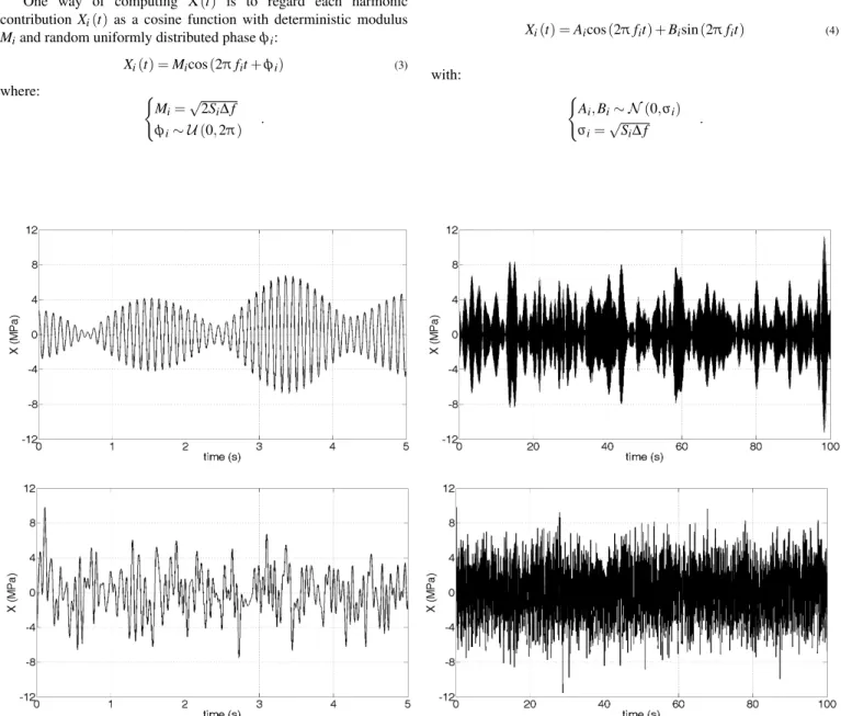
Figure 3: Process samples during a short (left) and a longer (right) time, narrow-band (top) and wide-band (bottom) PSDs.

It should be noted that processes generated from Eq. (3) considering deterministic moduli are asymptotically Gaussian when the number of frequency pointsnf tends to infinity, in virtue of the Central Limit Theorem. Besides, the use of Eq. (3) with Rayleigh distributed moduli is equivalent to the use of Eq. (4) with Gaussian amplitudes (Tucker, 1984). In the sequel, computations are performed using Eq. (4). One realization of the processes under consideration is shown in Fig. 3 to illustrate the narrow-band and wide-band concepts.

Numerical aspects

process is the sum of the variances of each harmonic contribution:

V[X(t)] = nf

∑

V[Xi(t)] = nf

∑

σi2= nf

∑

V[Xi] =V[X].

The temporal variable vanishes due to the expected stationarity of the process. However, the reader must keep in mind that empirical processes cannot be stationary if the number of frequenciesnf is not large enough. On the contrary, they are Gaussian for any number of frequencies since they are computed as a linear combination of Gaussian random variables. In addition, it can be shown that the processes under consideration are ergodic for the mean but not for the correlation function (see Appendix). Besides, each PSD is characterized by its central frequencyf0such as:

f0= 1 2π

r_m

2

m0

wheremkis the k-th order spectral moment, defined from the PSD by:

mk= Z +∞

0

(2πf)kS(f)df.

We recall that the PSD S(f)is one-sided and involves the frequency variable. For PSDs derived in terms of the circular frequency variable and/or two-sided, the previous expression is to be adapted. LetN0 denote the number of up-crossings of the zero threshold (i.e. the number of cycles) andT the time duration of the signals. We have the following relation:

N0=f0T.

Thus the knowledge of both the number of cycles and the PSD yields the samples duration. Moreover, it should be noted that the computed processes are periodic, due to the use of harmonic functions. So we make sure to adjust the time periodT to the samples length in order to avoid any duplication of the signals in the observation window. In practice, the value ofT must be large enough to cover 106 cycles considering high cycle fatigue applications. Then a large number of frequencies are needed, which makes the frequency step∆f being very small and the generation time-consuming. One way to solve this problem is to take advantage of the IFFT algorithm. As matter of fact, adapting Eq. (4), we have:

X(t) = nf

∑

Aicos(2πfit) +Bisin(2πfit)

= nf

∑

Aicos(2πfit) +Bicos

−π 2+2πfit

= nf

∑

AiRe

h

ej2πfiti_+B iRe

h

e−jπ2_ej2πfiti

= Re

"_n

f

∑

(Ai−Bi)ej2πfit

#

= nf

∑

(Ai−Bi)ej2πfit.

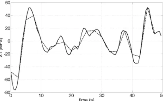
The real operator vanishes since the calculations yield an inverse Fourier transform whose result is real-valued. This transform can be rapidly computed using theifftfunction implemented in Matlab. On top of that, computing extreme value distributions requires accurate peaks in the temporal signals, which is conditioned by a refined sampling, as shown in Fig. 4. To get enough time points, we

perform a zero-padding up to 100 Hz in the frequency domain. Indeed, due to the use of the IFFT algorithm, the number of sampling points is the same in both the time and the frequency domains. nf =105 frequencies are used in the narrow-band case andnf =2.106frequencies are used in the wide-band case. To get accurate distributions, 104_{realizations of the processes are required.} Complying with the last remarks leads to dealing with a huge amount of data. Generating 104_{narrow-band samples requires 7h15 user time} using Matlab 7.11 without any specific launch options on a Linux server having 24 processors Intel(R) Xeon(R) CPU X5680 cadenced at 3.33 GHz with 12 MB cached size and 192 GB total memory. In comparison, nearly 115h are needed when using thefilter function implemented in Matlab to generate the same Gaussian processes via AR series.

Figure 4: Importance of temporal discretization.

Results analysis

To verify the adequateness of the computed samples, the empirical auto-correlation coefficient is calculated and compared to the analytical one in Fig. 5. For stationary processes, the auto-correlation coefficient is defined as:

ρ(τ) =R(τ)

V[X]. (5)

R(τ)being the auto-correlation function defined as:

R(τ) =E[X(t)X(t+τ)],t∈[0,T] (6)

whereτis the time shift between the two instantstandt+τinvolved in Eq. (6), E[•]being the mean operator. Note thatτ_∈[−T,T]. Due to Eq. (1), in both the low-pass and the band-pass cases, the auto-correlation function is given by:

R(τ) = S0 2π

sin(2πf2τ)−sin(2πf1τ)

τ . (7)

Table 1: Comparison between the theoretical and the empirical variances, narrow-band (top) and wide-band (bottom) cases.

Empirical (target) variance Relative gap

7.0082 (7) 0.12 %

Empirical (target) variance Relative gap

7.0037 (7) 0.05 %

Figure 5: Comparison between empirical and analytical auto-correlation coefficients, narrow-band (top) and wide-band (bottom).

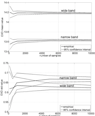
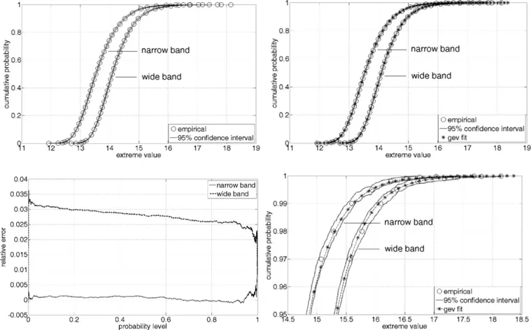
The greatest value of each realization is stored in order to compute the associated distribution. In the sequel, EVD stands for “extreme value distribution”. Different verifications are made to evaluate the quality of the empirical EVDs. First, its mean and standard deviation are computed for an increasing number of samples. The values are provided in Fig. 6 with the related confidence intervals (95%), obtained from the bootstrap method. When generating 104samples of each process, the mean and standard deviation have converged, as well as the related confidence intervals. Secondly, the empirical EVD is plotted together with its 95% confidence interval, computed from the Greenwood formula. It must be underlined that this interval is extremely reduced, due to the large number of realizations. Finally, it is interesting to check (see Fig. 7) if the empirical EVDs actually “look like” usual EVDs. These are then fitted with 3 parameters Generalized Extreme Value (GEV) distributions:

F(x;ξ,µ,β) =exp

"

−

1+ξx−µ β

−1_ξ#

, 1+ξx−µ

β >0,ξ6=0 (8)

Figure 6: Convergence of the EVDs mean (top) and standard deviation (bottom) value.

In probability theory and statistics, the GEV distribution is a family of continuous probability distributions developed under the extreme value theory in order to combine the Gumbel, Fréchet and Weibull families. The parametrization involved in Eq. (8) results from the work of von Mises (1936) and Jenkinson (1955). The GEV distribution arises from the extreme value theorem (Fisher and Tippet, 1928) as the limiting distribution of properly normalized maxima of a sequence of independent and identically distributed random variables. It has been shown that the framework can be extended to Gaussian processes; see for example De Haan and Ferreira (2006). The above-mentioned GEV distribution is computed from the simulation results by means of the maximum likelihood method (gevfit function in Matlab). It should be noted that the resulting curve lies in the confidence interval. A particular attention is paid to the distribution tails since these may be involved in reliability calculations. We end by evaluating the relative errorerr(p)between the empirical CDF and the related GEV distribution for any probability level p, 0≤p≤1.

Letsth(p)be the threshold such that Prob

max

t_∈[0,T](X(t))<sth

=pin

the theoretical model (GEV, here). LetsMC(p)be the threshold such

that Prob

max

t_∈[0,T](X(t))<sMC

=pin the MC simulations. Then the

relative error is computed as follows:

err(p) =sth(p)−sMC(p)

sMC(p)

. (9)

Figure 7: Confidence interval of the EVDs and fit with GEV distributions.

Extension to the Multi-Dimensional Case

Both cases introduced in the previous paragraph are now generalized to several processes. Using the PSDs relative to then

processes to be considered, we have the spectral matrix:

S(f) =



   

S11(f) S12(f) ··· S1n(f) S21(f) S22(f) ··· S2n(f)

..

. ... . .. ... Sn1(f) Sn2(f) ··· Snn(f)



   

=



   

S11(f) S12(f) ··· S1n(f) S∗₁₂(f) S22(f) ··· S2n(f)

..

. ... . .. ... S∗_1n(f) S∗_2n(f) ··· Snn(f)



    .

Spp(f), p=1, . . . ,n being the process p auto-PSD and Spq(f), p,q= 1, . . . ,n being the cross-PSD between processes p and q. Each auto-PSD shows the variance frequential repartition of the related process. Each cross-PSD provides the covariance frequential repartition of the associated processes. In particular, we now consider the two-dimensional correlated case. Unlike the general case, cross-PSDs are real-valued in the following. As in the first section, the

academic case of band-limited white noise is considered:

S11(f) =

(

S01 iff∈(f1,f2] 0 else

S22(f) =

(

S02 iff∈(f1,f2] 0 else

S12(f) =

(

S012 iff∈(f1,f2] 0 else

. (10)

Analogously to the one-dimensional case:

• in the narrow-band case, we take f1 =9.5 Hz, f2 =10.5 Hz,S01=3 MPa2/Hz,S02=5 MPa2/Hz,S012=0.9√S01S02 MPa2/Hz;

• the wide-band case, we takef1=0 Hz,f2=20 Hz,S01=0.15 MPa2/Hz,S02=0.25 MPa2/Hz,S012=0.9

√

S01S02MPa2/Hz.

It should be noted that in either case,S01 is such that V[X1(t)] =3 MPa2, S02 is such that V[X2(t)] =5 MPa2 and S012 is such that

cov[X1(t),X2(t)]

√

V[X1(t)]V[X2(t)]

= 0.9, cov[X1(t),X2(t)] denoting the statistical

Figure 8: Narrow-band (top) and wide-band (bottom) PSDs of the investigated multi-dimensional case.

Analogously to the one-dimensional situation, for either case (wide and narrow) we proceed as follows: at first, 104realizations are generated by assuming that the processes are Gaussian. Afterwards, the bivariate extreme value distribution is estimated from these empirical data as well as the associated margins and empirical cross-correlation coefficient. Like in the previous Results analysis subsection, the marginal EVDs are fitted with GEV distributions. The latter are then used together with the cross-correlation coefficient in order to compute a theoretical bivariate distribution.

Theory of Gaussian processes generation

Here again, each realization of a Gaussian process results from a sum of harmonic functions of time with random amplitudes computed from the PSD. Compared to the one-dimensional case, the difference lies in the fact that random quantities have to be appropriately correlated such that processes are correlated according to their associated target cross-PSD. Then, Eq. (4) is generalized as follows:

Xp(t) = nf

∑

n=2

∑

Aipqcos 2πfit+θipq+Bipqsin 2πfit+θipq

(11) where:



        

        

Aipq=Aiq(fi)σipq Bipq=Biq(fi)σipq Aiq,Biq∼N(0,1)

σipq=

Hpq(fi)

√

∆f

θipq=argHpq(fi)

H(fi) =S(fi)

1 2

.

ibeing the frequency index,pbeing the current process index andq

being the summation index (pbeing fixed) on all the processes (to introduce correlation between Xpand Xq).

Results analysis

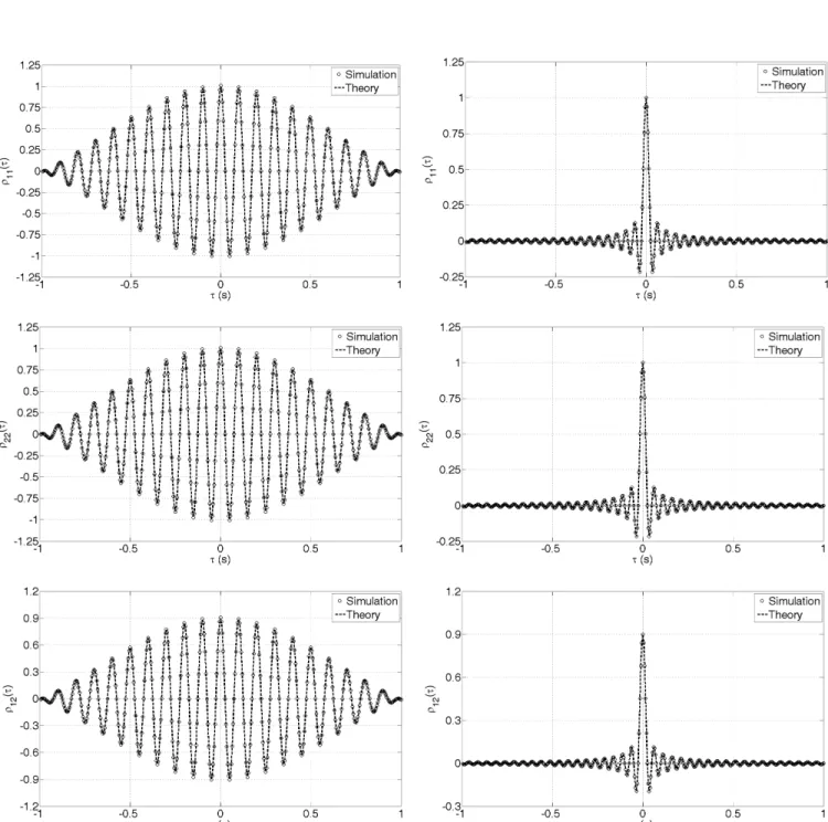
In order to verify the adequateness of the computed samples, the empirical auto and cross-correlation functions are calculated and compared to the analytical ones in Fig. 9. Analogously to Eq. (5), for a stationary process, the (auto and cross) correlation coefficients are defined as:

ρpq(τ) =

Rpq(τ) V

XpVXq

. (12)

Rpq(τ)being the related correlation function defined as:

Rpq(τ) =EXp(t)Xq(t+τ),t∈[0,T] (13)

whereτis the time shift between the two instantstandt+τinvolved in Eq. (13). As mentioned earlier,τ_∈[−T,T]. Using Eq. (11) in (13) yields:

Rpq(τ) = nf

∑

n

∑

Hpz(fi)Hqz(fi)

∆fcos 2πfitτ+θiqz−θipz.

(14) Due to Eq. (10), in both the low-pass and the band-pass cases, the correlation functions are given by:

R11(τ) =

S01 2π

sin(2πf2τ)−sin(2πf1τ) τ

R22(τ) =

S02 2π

sin(2πf2τ)−sin(2πf1τ)

τ (15)

R12(τ) =

Re[S012] 2π

sin(2πf2τ)−sin(2πf1τ) τ

+ Im[S012] 2π

cos(2πf2τ)−cos(2πf1τ)

τ .

Table 2: Comparison between the theoretical and the empirical variances and cross-correlation coefficients, narrow-band (top) and wide-band (bottom) cases.

Empirical (target) value Relative gap

V[X1] 3.0267 (3) 0.89%

V[X2] 5.0462 (5) 0.92%

ρ12 0.9082 (0.9) 0.91 %

Empirical (target) value Relative gap

V[X1] 2.9999 (3) -0.004%

V[X2] 5.0005 (5) 0.011%

ρ12 0.9001 (0.9) 0.008 %

In order to compare the empirical and analytical correlation coefficients in a proper way, both the empirical and analytical correlation functions are normalized using the theoretical values of the variances. To quantify the precision of the simulation, we are interested in comparing in detail the theoretical and empirical values of the variances and cross-correlation coefficients. nf = 102 _{frequencies are used in the narrow-band case and n}

f =2.103 frequencies are used in the wide-band case. We can see from Fig. 9 that the empirical auto and cross-correlation coefficients agree well with the analytical ones. Moreover, Table 2 shows that the empirical variances and cross-correlation coefficients of the computed processes are in total agreement with the theoretical ones. This implies that the simulated processes actually correspond to their respective target PSDs and are accurately correlated.

the one-dimensional case. These can be used to find the bivariate distribution. In the literature, Raynal-Villasenor and Salas (1987) and Elshamy (1992) present two differentiable models that are well suited for our study. From them, we consider the more flexible and widely applicable model:

Fm12(s1,s2) =exp

n

−[_{−ln[Fm1(s1)]}m+{−ln[Fm2(s2)]}m]

1

m

o

(16)

whereFmi(si)is the marginal EVD of the process Xi(t),Fm12(s1,s2) denotes the related bivariate EVD andmis the association parameter. It is such thatm∈[1,+∞[, wherem=1 gives the independence case and m_→+∞corresponds to a complete dependence between the margins. This parameter is a function of the correlation coefficient ρmbetween the marginal EVD:

m= (1−ρm)−

1

2_. (17)

Figure 10: Bivariate extreme value distributions, narrow-band (top) and wide-band (bottom) cases.

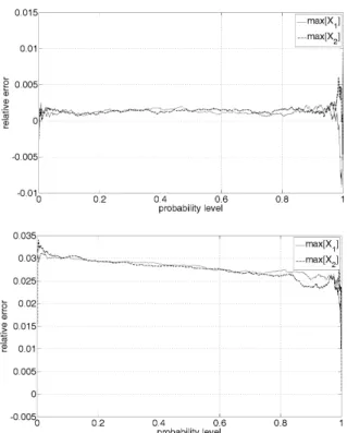
Figure 11: Relative error between the empirical margins and their GEV fits, narrow-band (top) and wide-band (bottom) cases.

In this work,ρm is obtained from empirical data using Matlab (corrcoef function). Then Eq. (16) can be used with the GEV fit of the margins. The resulting distribution fits very well the empirical bivariate EVD, as shown by Fig. 10. This arises since fitting the

extreme value margins with GEV distributions yields little errors (see Fig. 11).

Application Considering an Hydrology Spectrum

Input data

Here we consider mechanical stresses involved in a combination of a traction and a torsion loading, respectivelySxx(t) andSxy(t). Other components of the stress tensor are considered equal to zero. In the following, instead of simulatingSxx(t)andSxy(t), we generate the associated stresses processes needed for a fatigue criterion (Lambert et al., 2010):

(

X1(t) =

√

3 3 Sxx(t) X2(t) =Sxy(t)

.

Statistical moments are supposed to be the following:



   

   

E[Sxx(t)] =0MPa E

Sxy(t)=0MPa V[Sxx(t)] =2700MPa2 V

Sxy(t)

=675MPa2

⇒



   

   

E[X1(t)] =0MPa E[X2(t)] =0MPa V[X1(t)] =900MPa2 V[X2(t)] =675MPa2

.

The previous considerations will now be applied to a realistic example which may be related to a tidal stream turbine. In this case, the mechanical stresses PSDs may be of the following type:







Spq(f) =2π Apq (2πf)5e

− 3.11

(2πf)4_×82

f>0

Spq(f) =0 f=0

. (18)

Equation (18) represents a Bretschneider spectrum and is illustrated in Fig. 12. This kind of PSD is often encountered in the field of hydrology (Dalrymple, 1994). The values of the constantsApq are set as follows: A11 =174.94 S.I. units, A22 =131.21 S.I. units,

A12=136.35 S.I. units. It should be noted that in either case,A11 is such that V[X1(t)] =900 MPa2,A22is such that V[X2(t)] =675 MPa2andA12 is such that √cov[X1(t),X2(t)]

V[X1(t)]V[X2(t)]

=0.9. This situation is

represented in Fig. 12.

Figure 12: PSDs of the interested hydrology case.

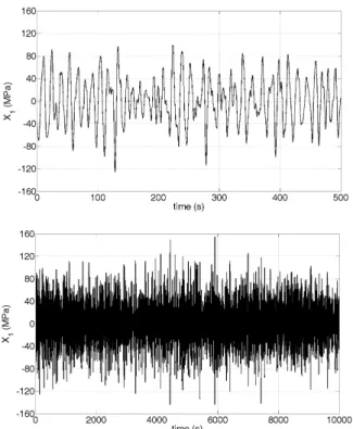
Figure 13: Process (X1) sample during a short (top) and a longer (bottom)

time.

Results analysis

In order to verify the adequateness of the computed samples, the empirical auto and cross-correlation functions are compared to the analytical ones in Fig. 14. nf =104 frequencies are used. Equations (12) to (14) are still valid in this situation. To compare the empirical and analytical correlation coefficients in a proper way, both the empirical and analytical correlation functions are normalized using the theoretical values of the variances. Due to the complexity of the involved PSDs, the analytical correlation functions cannot be evaluated analytically but they are computed by means of the IFFT algorithm. To quantify the precision of the simulation, let us compare in detail the theoretical and empirical values of the variances and cross-correlation coefficients. From Fig. 14, the empirical correlation coefficients agree well with the analytical ones. Moreover, Table 3 shows that the variances and cross-correlation coefficient of the computed processes are in total agreement with the theoretical values. This implies that the simulated processes actually correspond to their respective target PSDs and are correctly correlated.

As we did in the previous subsection Results analysis, marginal EVDs are fitted by GEV distributions. Figure 15 shows that the relative error is low. Then Eq. (16) can be used with the GEV approximations of the margins. The resulting distribution fits very well the empirical bivariate EVD, as shown by Fig. 16.

Table 3: Comparison between the theoretical and the empirical variances and cross-correlation coefficients.

Empirical (target) value Relative gap V[X1] 899.7903 (900) -0.0233 % V[X2] 674.7338 (675) -0.0394 %

ρ12 0.8997 (0.9) -0.0325 %

Figure 14: Comparison between empirical and analytical correlation coefficients.

Figure 16: Bivariate extreme value distributions.

Conclusions and Perspectives

We have presented an appropriate generation method for correlated Gaussian processes, dealing quite fast with a great amount of data thanks to the use of the IFFT algorithm. Moreover, it is able to give the processes extreme value distributions (univariate and multivariate) with a good quality, having a great confidence interval. Fitting the extreme value margins with GEV distributions provides excellent approximations and the model chosen for building the bivariate extreme value distribution is accurate. With this result, the structural reliability can then be evaluated by estimating the equivalent shear stress that is involved in multiaxial fatigue criteria; see Lambert et al. (2010) for an example of such an approach.

However, the bivariate extreme value distribution model involves the associated margins (or here their GEV fits) as well as the extreme value cross-correlation coefficient. Both these quantities are currently known from Monte-Carlo simulations, which are still time-consuming. Further work is then to be carried out to evaluate the cross-correlation coefficient of the extreme value distribution directly from the spectral description of the related processes. The same remark holds for the parameters of the GEV distributions fitting the margins. The influence parameters may be the spectral shapes and moments of the involved PSDs as well as the samples duration. The extension of the presented model for building bivariate EVD to more than two processes is also to be considered in order to deal with up to six-dimensional stress fields.

Appendix

Ergodicity for the mean

For more convenience, we introduceωi=2πfiin the following statements. At any given timet, the mathematical expectation of the process Xp(t)is:

µxp(t) =E

Xp(t)

= nf

∑

n

∑

σipqEAiqcos ωit+θipq

+E

Biqsin ωit+θipq =0.

For any given realization of the process Xp(t), the temporal mean is:

µx(rp)= 1

T nf

∑

n

∑

σipq

A(_iqr)

ZT

0 cos ωit+θipq

dt

+B(_iqr) ZT

0

sin ωit+θipqdt

=0.

Both the mathematical expectation and the temporal mean are equal (to zero), hence the processes are ergodic for the mean value.

Non ergodicity for the correlation function

At any given time t, the correlation function between the processes Xp(t)and Xz(t)is:

Rpz(τ) =EXp(t)Xz(t+τ)

= nf

∑

nf

∑

n

∑

n

∑

σi1pq1σi2zq2

×

E

Ai1q1Ai2q2

cos ωi1t+θi1pq1

cos ωi2(t+τ) +θi2zq2

+E

Ai1q1Bi2q2

cos ωi1t+θi1pq1

sin ωi2(t+τ) +θi2zq2

+E

Bi1q1Ai2q2

sin ωi1t+θi1pq1

cos ωi2(t+τ) +θi2zq2

+E

Bi1q1Bi2q2

sin ωi1t+θi1pq1

sin ωi2(t+τ) +θi2zq2

= nf

∑

n

∑

σipqσizq

×nEhA2_iqicos ωit+θipq

cos ωi(t+τ) +θizq

+EhB2iq

i

sin ωit+θipq

sin ωi(t+τ) +θizq

o .

SinceAiq andBiq are zero-mean random variables, their mean

square values are equal to their (unit) variances EhA2_iq i

=EhB2_iq i

=1. This yields:

Rpz(τ) = nf

∑

n

∑

σipqσizqcos ωit+θipqcos ωi(t+τ) +θizq

+sin ωit+θipq

sin ωi(t+τ) +θizq

= nf

∑

n

∑

σipqσizqcos ωitτ+θizq−θipq

.

For any given realization of the processes Xp(t) and Xz(t), the temporal correlation function is:

R(pzr)(τ) =

D

X(pr)(t)Xz(r)(t+τ)

E

=1

T ZT

0

X(pr)(t)Xz(r)(t+τ)dt

=1

T nf

∑

i1=1

nf

∑

i2=1

n

∑

q1=1

n

∑

q2=1

σi1pq1σi2zq2

×

A(_ir)

1q1A

(r) i2q2

ZT

0 cos ωi1t+θi1pq1

cos ωi2(t+τ) +θi2zq2

dt

+A(i1r)q1B

(r) i2q2

ZT

0 cos

ωi1t+θi1pq1

sin ωi2(t+τ) +θi2zq2

dt

+B(_ir)

1q1A

(r) i2q2

ZT

0

sin ωi1t+θi1pq1

cos ωi2(t+τ) +θi2zq2

dt

+B(_ir)

1q1B

(r) i2q2

ZT

0

sin ωi1t+θi1pq1

sin ωi2(t+τ) +θi2zq2

dt =1 T nf

∑

i1=1

nf

∑

i2=1

n

∑

q1=1

n

∑

q2=1

σi1pq1σi2zq2

×nA(_ir)

1q1A

(r) i2q2I1+A

(r) i1q1B

(r) i2q2I2+B

(r) i1q1A

(r) i2q2I3+B

(r) i1q1B

(r) i2q2I4

o

After some calculations, we find:

I1= 1 2

ZT

0 cos (ωi1−ωi2)t−ωi2τ+θi1pq1−θi2zq2

dt

I2=− 1 2

ZT

0

sin (ωi1−ωi2)t−ωi2τ+θi1pq1−θi2zq2

dt

I3= 1 2

ZT

0

sin (ωi1−ωi2)t−ωi2τ+θi1pq1−θi2zq2

dt

I4= 1 2

ZT

0 cos (ωi1−ωi2)t−ωi2τ+θi1pq1−θi2zq2

dt.

ReplacingI1toI4by their respective expressions gives:

R(pzr)(τ) =1 T

nf

∑

i1=1

nf

∑

i2=1

n

∑

q1=1

n

∑

q2=1

σi1pq1σi2zq2

× 





A(i1r)q1A

(r) i2q2+B

(r) i1q1B

(r) i2q2

2

ZT

0 cos ωi1−ωi2

t−ωi2τ+θi1pq1−θi2zq2

dt

+ B

(r) i1q1A

(r) i2q2−A

(r) i1q1B

(r) i2q2

2

ZT

0 sin ωi1−ωi2

t−ωi2τ+θi1pq1−θi2zq2

dt    = 1 T nf

∑

i=1

n

∑

q=1

σipqσizq

A(_iqr)2+B(_iqr)2 2

ZT

0 cos −

ωiτ+θipq−θizqdt

= nf

∑

i=1

n

∑

q=1

σipqσizq

A(_iqr)2+B(_iqr)2

2 cos ωiτ+θizq−θipq

.

Both the mathematical expectation and the temporal mean are not equal, hence the processes are not ergodic for the correlation function.

References

Dalrymple, R.A., 1994, “The theory of short-period waves,” in M.B. Abbott and W.A. Price, editors, Coastal, estuarial, and harbour engineers’ reference book, pp. 37-44.

De Haan, L. and Ferreira, A., 2006, “Extreme Value Theory: An Introduction,” Springer, Ch. 9.

Elshamy, M., 1992, “Bivariate extreme value distributions,” NASA Contractor Report No. 4444.

Fisher, R.A. and Tippet L.H.C., 1928, “Limiting forms of the frequency distribution of the largest and smallest member of a sample,” Proceedings of the Cambridge Philosophical Society, Vol. 24, pp. 180-190.

Gmür, T., 1997, “Dynamique des structures: analyse modale numérique,” Presses polytechniques et universitaires romandes, Ch. 2-3.

Guéna, F., Daviau, J.F., Majastre, H., Bischoff, V., Ruer, J. and Tartivel, C., 2006, “Design and operational features of a tidal stream turbine,” Proceedings of the European Seminar on Offshore Wind and Other Marine Renewable Energies in Mediterranean and European Seas, OWEMES, Civitavecchia, Italy, 22nd April 2006, 8p.

Jenkinson, A.F., 1955, “The frequency distribution of the annual maximum (or minimum) values of meteorological elements,” Quarterly

Journal of the Royal Meteorological Society, John Wiley & Sons, Ltd, Vol.

81, pp 158-171.

Khalij, L., Pagnacco, E. and Lambert, S., (2010) “A measure of the equivalent shear stress amplitude from a prismatic hull in the principal coordinate system,”International Journal of Fatigue, Vol. 32, No. 12, pp. 1977-1984.

Lambert, S., Pagnacco, E. and Khalij, L., 2010, “A probabilistic model for the fatigue reliability of structures under random loadings with phase shift effects,”International Journal of Fatigue, Vol. 32, No. 2, pp. 463-474.

von Mises, R., 1936. “La distribution de la plus grande de n valeurs,” reprinted in Selected Papers Volumen II, American Mathematical Society, Providence, R.I., 1954, pp. 271-294.

Raynal-Villasenor, J.A. and Salas, J.D., 1987, “Multivariate extreme value distributions in hydrological analyses.” Proceedings of the Rome Symposium on “Water for the future: hydrology in perspective”, IAHS Publ. No. 164, 10p.

Sun, J.Q., 2006, “Stochastic dynamics and control,” in J.-Q. Sun, editor, Stochastic Dynamics and Control, Vol. 4 of Monograph Series on Nonlinear Science and Complexity, pp.229-235.

Theodorsen, T., 1934, “General theory of aerodynamic instability and the mechanism of flutter,” National Advisory Committee for Aeronautics Report No. 496.

Thresher, R.W., Mirandy, L.P., Carne, T.G., Lobitz, D.W. and James, G.H., 2009, “Chapter 11: Structural dynamic behavior of wind turbines,” Spera, D. A., ed. New York: American Society of Mechanical Engineers (ASME) pp. 605-662; NREL Report No. CH-500-45391.