PLASIM-ENTSem: a spatio-temporal emulator of future climate change for impacts assessment

(1)

GMDD

6, 3349–3380, 2013

PLASIM-ENTS climate emulator

P. B. Holden et al.

Title Page

Abstract Introduction

Conclusions References

Tables Figures

◭ ◮

Back Close

Full Screen / Esc

Printer-friendly Version Interactive Discussion

Discussion

P

a

per

|

D

iscussion

P

a

per

|

Discussion

P

a

per

|

Discuss

ion

P

a

per

|

Geosci. Model Dev. Discuss., 6, 3349–3380, 2013 www.geosci-model-dev-discuss.net/6/3349/2013/ doi:10.5194/gmdd-6-3349-2013

Geoscientiic Geoscientiic

Geoscientiic

Open Access

Geoscientiic Model Development

Discussions

This discussion paper is/has been under review for the journal Geoscientific Model Development (GMD). Please refer to the corresponding final paper in GMD if available.

PLASIM-ENTSem: a spatio-temporal

emulator of future climate change for

impacts assessment

P. B. Holden1, N. R. Edwards1, P. H. Garthwaite2, K. Fraedrich3, F. Lunkeit3,

E. Kirk3, M. Labriet4, A. Kanudia4, and F. Babonneau5

1

Earth, Environment and Ecosystems, Open University, UK

2

Mathematics and Statistics, Open University, UK

3

Meteorologisches Institut, Universität Hamburg, Hamburg, Germany

4

Eneris Environment Energy Consultants, Madrid, Spain

5

ORDECSYS, Chêne-Bougeries, Switzerland and REME Laboratory, Swiss Federal Institute of Technology at Lausanne (EPFL), Lausanne, Switzerland

Received: 14 May 2013 – Accepted: 6 June 2013 – Published: 25 June 2013

Correspondence to: P. B. Holden (philip.holden@open.ac.uk)

(2)

GMDD

6, 3349–3380, 2013

P. B. Holden et al.

Title Page

Tables Figures

◭ ◮

Back Close

Full Screen / Esc

Discussion

P

a

per

|

D

iscussion

P

a

per

|

Discussion

P

a

per

|

Discuss

ion

P

a

per

|

Abstract

Many applications in the evaluation of climate impacts and environmental policy re-quire detailed spatio-temporal projections of future climate. To capture feedbacks from impacted natural or socio-economic systems requires interactive two-way coupling but this is generally computationally infeasible with even moderately complex general

cir-5

culation models (GCMs). Dimension reduction using emulation is one solution to this problem, demonstrated here with the GCM PLASIM-ENTS. Our approach generates temporally evolving spatial patterns of climate variables, considering multiple modes of variability in order to capture non-linear feedbacks. The emulator provides a 188-member ensemble of decadally and spatially resolved (_∼5◦ resolution) seasonal

cli-10

mate data in response to an arbitrary future CO2 concentration and radiative forcing

scenario. We present the PLASIM-ENTS coupled model, the construction of its emu-lator from an ensemble of transient future simulations, an application of the emuemu-lator methodology to produce heating and cooling degree-day projections, and the validation of the results against empirical data and higher-complexity models. We also

demon-15

strate the application to estimates of sea-level rise and associated uncertainty.

1 Introduction

Emulators are widely used tools to inexpensively estimate expensive simulator output. They are generally used to calibrate input parameters or to estimate the uncertainty associated with a prediction (O’Hagan, 2006). The standard emulation approach uses

20

a Gaussian process (Santner et al., 2003), conditioned on simulations at different in-puts. This can then be used to predict the model response at a new set of inputs, together with an evaluation of the uncertainty of that prediction. This uncertainty rep-resents an estimate of the error associated with the emulation process and is termed “code uncertainty” (O’Hagan, 2006). A second source of uncertainty in the prediction

25

(3)

GMDD

6, 3349–3380, 2013

P. B. Holden et al.

Title Page

Tables Figures

◭ ◮

Back Close

Full Screen / Esc

Discussion

P

a

per

|

D

iscussion

P

a

per

|

Discussion

P

a

per

|

Discuss

ion

P

a

per

|

from an uncertain knowledge of “best” simulator inputs and, when the simulator is too expensive, can be evaluated from the emulated response over plausible input space. When parametric error dominates over code uncertainty, relatively simple emulation techniques (that do not attempt to evaluate code uncertainty through a Gaussian pro-cess) are appropriate for an evaluation of simulated parametric uncertainty (Holden

5

et al., 2010; Holden and Edwards, 2010; Edwards et al., 2011).

The extension of emulation techniques to consider multivariate outputs using ap-proaches that can capture the correlations between the outputs have been devel-oped (Rougier, 2008; Conti and O’Hagan, 2010). However, these approaches are not well suited to the emulation of very high-dimensional output, although Rougier (2008)

10

made advances in this regard by factorising the covariance matrix, and data reduction methods may be required to reduce the size of a problem (Wilkinson, 2011). Holden and Edwards (2010) applied this data reduction approach, using principal component analysis to project_∼1000-dimensional climate model output onto a lower dimensional space and then emulating the map from the input space to the lower dimensional

out-15

put space. We here extend Holden and Edwards (2010) to develop a spatio-temporal climate model emulator for applications to impact assessment.

One of the principal obstacles to coupling complex climate and impact models is that the inclusion of feedbacks can induce a multiplier on the overall computational cost that renders the problem intractable. The conventional way to address this intractability

20

is to use pattern scaling (Mitchell et al., 1999). However, replacing the climate model with an emulated version of its input-output response function represents a substantial advance on pattern scaling by retaining the possibility of including non-linear spatio-temporal feedbacks and uncertainty (Holden and Edwards, 2010). In addition to speed, this approach yields two further benefits in the field of integrated assessments. First,

25

(4)

GMDD

6, 3349–3380, 2013

P. B. Holden et al.

Title Page

Tables Figures

◭ ◮

Back Close

Full Screen / Esc

Discussion

P

a

per

|

D

iscussion

P

a

per

|

Discussion

P

a

per

|

Discuss

ion

P

a

per

|

The potential benefits of an approach using emulation have been discussed in some detail in Holden and Edwards (2010). However, several limitations of this earlier emula-tor have restricted possible coupling applications. Firstly, the emulation was applied to the intermediate complexity atmosphere-ocean GCM GENIE-2 (Lenton et al., 2007). The precipitation fields in that model are known to contain structural biases (Annan

5

et al., 2005) and numerical artefacts, making it an unsatisfactory tool for impacts cal-culations. In order to address this we have developed a new climate model, the Planet Simulator PLASIM (Fraedrich, 2012; Fraedrich et al., 2005a) with the terrestrial car-bon and land-surface model ENTS (Williamson et al., 2006). Secondly, the Holden and Edwards (2010) emulator was limited to spatial predictions at a single time-slice. Here

10

a single emulator calculation is used to derive an entire, self-consistent, decadally re-solved temporal history of each output field.

After presenting the new PLASIM-ENTS coupled model in Sect. 2, we describe the ensemble design in Sect. 3. In Sect. 4 we describe the emulation of seasonally re-solved temperature and temperature variability fields, from which heating and cooling

15

degree-days are derived for impact calculations in Sect. 5. Model validation is covered in Sect. 6, while conclusions are discussed in Sect. 7.

2 The climate model: PLASIM-ENTS

The climate model used here is the Planet Simulator (PLASIM, Fraedrich, 2012; Fraedrich et al., 2005a), Version 16 Revision 4, with adaptations described below,

20

most notably the incorporation of an alternative representation of terrestrial vegetation. PLASIM is an intermediate complexity General Circulation Model (GCM) built around the 3-D dynamical atmosphere PUMA (Fraedrich et al., 2005b). We run the model at T21 resolution (_∼5.6◦_×5.6◦) with ten vertical levels.

The Planet Simulator (freely available under http://www.mi.uni-hamburg.de/plasim)

25

(5)

GMDD

6, 3349–3380, 2013

P. B. Holden et al.

Title Page

Tables Figures

◭ ◮

Back Close

Full Screen / Esc

Discussion

P

a

per

|

D

iscussion

P

a

per

|

Discussion

P

a

per

|

Discuss

ion

P

a

per

|

a desert world versus green planet (Fraedrich et al., 2005b), the entropy budget and its sensitivity (Fraedrich and Lunkeit, 2008), the global energy and entropy budget in a snowball Earth hysteresis (Lucarini et al., 2010), and the double ITCZ dynamics in an aquaplanet setup (Dahms et al., 2011). This model is being employed to reconstruct historic climates (Grosfeld et al., 2007), to determine the younger history of the Andean

5

uplift (Garreaud et al., 2010), to analyse the effect of mountains on the ocean circula-tion (Schmittner et al., 2011), and to evaluate biogeophysical feedbacks (Dekker et al., 2010; Bathiani et al., 2013). Furthermore, it enables investigations of climates very dif-ferent from recent Earth conditions as shown in applications for Mars with and without ice (Stenzel et al., 2007), the Neoproterozoic snowball earth (Micheels and Montenari,

10

2008), and the Permian climates (Roschner et al., 2011). For recent climate change related analyses see Bordi et al. (2011a,b, 2013).

The atmospheric dynamics (described in detail in above references) is based on primitive equations formulated for vorticity, divergence, temperature and the logarithm of surface pressure, solved via the spectral transform method. The parameterizations

15

for unresolved processes consist of long and short wave radiation. The model takes into account only water vapour, carbon dioxide and ozone as greenhouse gases. The ozone concentration is prescribed according to an analytic ozone vertical distribution. The annual cycle and the latitudinal dependence are introduced. Further parameterizations are included for interactive clouds, moist and dry convection, large-scale precipitation,

20

boundary layer fluxes of latent and sensible heat and vertical and horizontal diffusion. The land surface scheme uses five diffusive layers for the temperature and a bucket model for the soil hydrology. The ocean is represented by a mixed layer (swamp) ocean, which includes a 0-dimensional thermodynamic sea ice model.

We have adapted the PLASIM land surface dynamics by the inclusion of the simple

25

land surface and vegetation model ENTS (Williamson et al., 2006). ENTS represents vegetative and soil carbon through a single plant functional type with photosynthesis a function of temperature, soil moisture availability, atmospheric CO2concentration and

(6)

GMDD

6, 3349–3380, 2013

P. B. Holden et al.

Title Page

Tables Figures

◭ ◮

Back Close

Full Screen / Esc

Discussion

P

a

per

|

D

iscussion

P

a

per

|

Discussion

P

a

per

|

Discuss

ion

P

a

per

|

capture the different responses of tropical and boreal forest. Land surface character-istics (albedo, surface roughness length and moisture bucket capacity) are diagnosed from the simulated state variables of vegetation and soil carbon densities. We note that land-atmosphere flux parameterisations are unchanged from those in PLASIM as these parameterisations in ENTS (Williamson et al., 2006) were developed for the

5

EMBM module of GENIE. Thus, in PLASIM-ENTS, we only incorporate the ENTS pa-rameterisations for vegetation and soil carbon densities and land surface character-istics. The motivation for using ENTS in this study, rather than the SIMBA vegetation model incorporated in PLASIM Version 16.4 (Kleidon, 2006) is that the ENTS model behaviour has been thoroughly investigated through previous ensemble experiments

10

(Holden et al., 2010, 2013a,b). The coupling was straightforward to implement given the structural similarities between ENTS and the default PLASIM vegetation model.

A number of minor modifications were made to the documented models described above. Firstly, we have introduced two new ENTS parameters, the optimum tempera-ture for photosynthesis and the threshold soil moistempera-ture required for photosynthesis.

15

The optimum temperature parameterTadj was introduced to allow for the uncertain

response of photosynthesis to future warming, which is associated with uncertainty in the climate-carbon feedback, especially in the tropics (Matthews et al., 2007). The surface temperatureT_a dependencies of photosynthesis in ENTS (Eqs. 19 and 20 of Williamson et al., 2006) are replaced throughout withTa+TadjwhereTadj(an input

pa-20

rameter that is varied across the ensemble described in Sect. 3) acts to shift the pho-tosynthesis diurnal average temperature optima from defaults of_∼8◦C and_∼31◦C.

The variable soil moisture threshold was introduced primarily to allow the simulation of vegetation in semi-arid regions that were not vegetated in the default PLASIM-ENTS coupling. This arises as the “wetness factor” in PLASIM, which acts to linearly scale

25

surface evaporation in order to inhibit evaporation from dry soils, is given byWs/0.4Ws∗

(whereWs is the soil moisture content andWs∗the bucket capacity), and takes its

max-imum value of unity whenWs/Ws∗≥0.4. This leads to drier soils than in the

GENIE-ENTS coupling, where the wetness factor is given by WS/WS∗

4

(7)

GMDD

6, 3349–3380, 2013

P. B. Holden et al.

Title Page

Tables Figures

◭ ◮

Back Close

Full Screen / Esc

Discussion

P

a

per

|

D

iscussion

P

a

per

|

Discussion

P

a

per

|

Discuss

ion

P

a

per

|

et al., 2006). The drier soils inhibit the growth of vegetation in PLASIM-ENTS using the standard ENTS parameterisations. To address this, the functional dependency of photosynthesis on soil moisture in PLASIM-ENTS has been altered to

f2(Ws)=

1/(0.75−qth)

Ws/Ws∗

−qth (1)

wheref2(Ws) is restricted to values between 0 (Ws/Ws∗≤qth) and 1 (Ws/Ws∗≥0.75).

5

The expression reduces to the standard ENTS parameterisation (Eq. 17 of Williamson et al., 2006) when the threshold fractional moistureqth=0.5. In the ensembles

per-formed here (see Sect. 3),qthis allowed to vary over the range 0.1 to 0.5.

The extent of modern sea ice is significantly overstated in the default PLASIM model. Sea-ice flux corrections are derived from fixed sea-ice spin-up simulations forced with

10

climatological sea-ice coverage. However, during these spin-ups, the default PLASIM configuration assumes 100 % sea-ice coverage in any grid cell with non-zero clima-tological ice cover. This then leads to overstated modern day sea-ice in the dynamic flux-corrected mode, and an unreasonably strong sea-ice feedback. The fixed sea-ice configuration has been changed so that sea ice is assumed to be present only when the

15

climatological grid cell-averaged sea-ice thickness exceeds some threshold, a variable in the ensemble (Sect. 3).

The sea ice was found to be unstable in flux corrected mode. This is likely a conse-quence of the fact that sea-ice coverage within a grid cell only takes values of zero or 100 %. Natural variability can lead to the establishment of instantaneous sea-ice

cover-20

age across an entire grid cell that may be stabilised due to the local albedo feedback. The result is that the sea-ice extent can drift towards greater coverage leading to an overestimate of modern day sea-ice coverage. In an attempt to address this, a simple parameterisation was introduced for the latitudinal dependence of ocean albedo, repre-senting the increased albedo of high latitude ocean and hence the reduced differential

25

between sea ice and ocean albedo. The simple parameterisation applied is

(8)

GMDD

6, 3349–3380, 2013

P. B. Holden et al.

Title Page

Tables Figures

◭ ◮

Back Close

Full Screen / Esc

Discussion

P

a

per

|

D

iscussion

P

a

per

|

Discussion

P

a

per

|

Discuss

ion

P

a

per

|

where the ocean albedoαsis expressed in terms of latitudeφ, the albedo at the

equa-tor αs0 (0.03) and the variable parameter αs1. Although we have not performed the

ensemble of simulations that would allow us to quantify the degree to which this may have improved sea-ice stability, the latitudinally dependent ocean albedo parameter-isation did not eliminate the sea-ice instability. The parameterparameter-isation is nonetheless

5

useful as a more faithful representation of the latitudinal balance of shortwave radia-tion. The sea-ice drift in PLASIM-ENTS is largely limited to the Southern Ocean, likely because climatological Arctic sea ice is thicker and exhibits less seasonal variability than Antarctic sea ice. The compromise ultimately adopted here was to simulate flux-corrected dynamic sea ice in the Arctic, but fixed sea ice in the Antarctic. Thus the

10

simulations capture the feedback associated with Arctic sea ice (important for North-ern Hemisphere impacts) without the bias introduced by the SouthNorth-ern Ocean sea-ice drift.

A number of input/output modifications were also made, being the addition of netcdf output routines, the diagnosis of seasonally averaged land-surface variables and

15

the automated runtime generation of ocean and sea-ice flux-corrections. Finally, the radiative-transfer scheme in PLASIM only allows for CO₂. We adapted the model to take two time-varying inputs: equivalent CO2, the concentration that is equivalent to

a given total radiative forcing (for provision to the radiative balance calculation) and actual CO₂(for input to ENTS for CO₂fertilisation).

20

3 Ensemble design

The philosophy for the design process has been described in detail elsewhere (Holden et al., 2010). In short, the approach attempts to vary key model parameters over the entire range of plausible input values and to accept parameter combinations which lead to climate states that cannot be un-controversially ruled out as implausible

(Ed-25

(9)

GMDD

6, 3349–3380, 2013

P. B. Holden et al.

Title Page

Tables Figures

◭ ◮

Back Close

Full Screen / Esc

Discussion

P

a

per

|

D

iscussion

P

a

per

|

Discussion

P

a

per

|

Discuss

ion

P

a

per

|

of the model from all regions of the high-dimensional input parameter space in order to capture the range of possible feedback strengths.

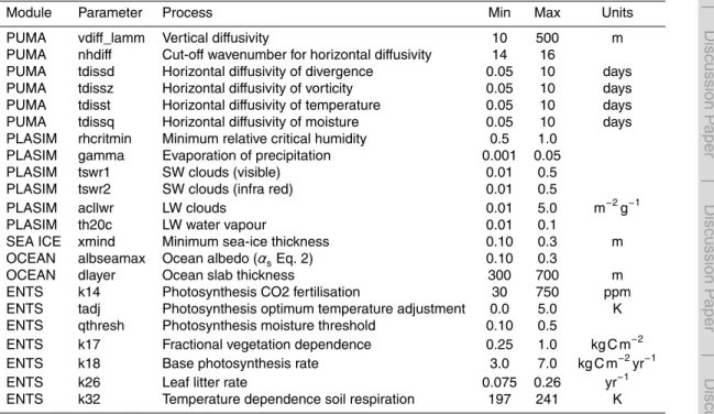
Following a series of exploratory ensembles, twenty-two key model parameters were selected with input ranges that are summarised in Table 1. Twelve of these parameters were chosen to capture uncertainties in atmospheric transport and in the atmospheric

5

radiative balance. The sea-ice parameterxmindwas varied to provide a range of mod-ern sea-ice configurations (global annually-averaged preindustrial coverage varying between∼21 and 27 million km2); this variability across the ensemble is designed as a proxy to generate uncertainty in the strength of the sea-ice feedback. Mixed layer thickness was varied to capture uncertain ocean heat capacity and thermal inertia.

10

The three new parameters introduced in Sect. 2, describing ocean albedo and the un-certain vegetation response to temperature and moisture availability, were varied, in addition to five key ENTS parameters, as previously identified in Holden et al. (2013a). In order to investigate the regions of this 22-dimensional parameter space that pro-duce plausible climate simulations, the parameters were first varied over their maximum

15

plausible ranges (Table 1) to create a 500-member Maximin Latin Hypercube (MLH) design, using the maximinLHS function of the lhs package in R (R development Core Team, 2013). The points of this experimental design (corresponding to sets of input pa-rameter values for PLASIM-ENTS) were used to generate a 500-member ensemble of 200 yr spun-up preindustrial simulations (with climatologically prescribed sea surface

20

temperatures and sea-ice coverage). These simulations were then used to generate scalar emulators for key global model outputs (surface air temperature, precipitation, top-of-atmosphere energy balance, vegetative carbon and soil carbon). The emulators were built performing stepwise regression including linear, quadratic and cross-terms for all 22 parameters using the stepAIC function (Venables and Ripley, 2002), following

25

the procedure described in Holden et al. (2010).

(10)

GMDD

6, 3349–3380, 2013

P. B. Holden et al.

Title Page

Tables Figures

◭ ◮

Back Close

Full Screen / Esc

Discussion

P

a

per

|

D

iscussion

P

a

per

|

Discussion

P

a

per

|

Discuss

ion

P

a

per

|

sets which the emulators predicted would lead to a reasonable model state, defined as global surface air temperature in the range 11 to 13◦C, precipitation (1025 to 1075 mm yr−1), top-of-atmosphere energy balance (₋3 to 3 W m−2), vegetation carbon (450 to 650 GTC)andsoil carbon (1000 to 2000 GTC). We note that an arbitrary choice of parameter values will not, in general, produce a reasonable climate state thus

ne-5

cessitating the use of the emulators in the design process. (Only ten of the five hundred parameter sets in the design MLH ensemble produced a plausible climate state.)

3.1 Historical transients

The MPEF parameter sets were used as inputs for transient simulations with historical radiative forcing from 1765 to 2005 of http://www.pik-potsdam.de/~mmalte/rcps/.

Tem-10

porally varying, globally averaged radiative forcing was provided, converted into equiv-alent CO2, together with actual CO2concentration for vegetation input. Each simulation

was initially run to equilibrium with preindustrial forcing, assuming PMIP II sea surface temperature and sea-ice distributions (monthly averages over the whole time period 1870 to 2006, http://www-pcmdi.llnl.gov/projects/amip). Monthly ocean and sea-ice flux

15

corrections were diagnosed from these equilibrium states. The dynamic flux-corrected mixed layer ocean was applied in these historical transients but sea ice was held fixed globally. The simulations were subjected to four present day (2005 AD) plausibility tests: global average land temperature (required to be in the range 11.5 to 13.5◦C), global average precipitation (1000 to 1100 mm yr−1), total vegetative carbon (400 to

20

700 GTC) and total soil carbon (800 to 2200 GTC). Additionally, the top-of-atmosphere energy balance was required to be in approximate equilibrium (−5 to 5 W m−2) in the initialised preindustrial state. On the basis of these five tests, 188 simulations were accepted for the future forced experiments, forming the “Modern-Plausible-Simulator -Filtered” MPSF parameter set.

(11)

GMDD

6, 3349–3380, 2013

P. B. Holden et al.

Title Page

Tables Figures

◭ ◮

Back Close

Full Screen / Esc

Discussion

P

a

per

|

D

iscussion

P

a

per

|

Discussion

P

a

per

|

Discuss

ion

P

a

per

|

3.2 Future ensemble

For the future transient simulations, the experimental configuration was changed to model dynamic, flux-corrected Arctic sea ice, but retaining fixed sea ice in the Antarctic (see Sect. 2). The motivation for this came from two exploratory ensembles. The first, with globally fixed sea ice, was found to greatly understate polar amplification, with

im-5

plications for the evaluation of high-latitude impacts. The second, with globally dynamic sea ice, produced overstated present-day Antarctic sea ice, a cold-biased global tem-perature and excessive high-latitude southern warming in response to future forcing. The chosen compromise allows us to capture the uncertain response of Arctic sea ice, which is important for the evaluation of high-latitude Northern Hemisphere impacts.

10

Although Antarctic warming is somewhat understated in this experimental set-up, a mi-nor issue for the evaluation of societal impacts, the spatial and seasonal distribution of warming otherwise compares favourably to state-of-the-art GCM predictions (Sect. 6). Future radiative forcing (2005–2105) was expressed in terms of CO2equivalent

con-centration CO2e, with a temporal profile described by a linear decomposition of the 1st

15

three Chebyshev polynomials:

CO2e=C0e+0.5

n

A1e t+1

+A2e 2t2−2

+A3e 4t3−4t

o

(3)

where C0e is CO2e in 2005 (386.5 ppm), t is time (2005 to 2105) normalised onto the

range (₋1,1) and the three coefficients that describe the concentration profile (A_1e,A_2e

andA3e) take values that allow for a wide range of possible future emissions profiles (0

20

to 1000,₋200 to 200 and₋100 to 100 ppm, respectively). These ranges encompass the range of RCP scenarios (Meinshausen et al., 2009; Moss et al., 2010) with a CO2e

concentration in 2105 ranging from 387 to 1387 ppm. The motivation for the use of a Chebyshev polynomial is to facilitate emulation, by reducing (and hence approximat-ing) an arbitrary forcing profile to three orthogonal input coefficients.

(12)

GMDD

6, 3349–3380, 2013

P. B. Holden et al.

Title Page

Tables Figures

◭ ◮

Back Close

Full Screen / Esc

Discussion

P

a

per

|

D

iscussion

P

a

per

|

Discussion

P

a

per

|

Discuss

ion

P

a

per

|

The same approach was taken to describe the temporal profile of actual CO₂ (with C0=380.2 ppm):

CO2=C0+0.5

n

A1 t+1

+A2 2t2−2

+A3 4t3−4t

o

(4)

Each of the 188 MPSF 2005 spun-up states and parameter sets was used three times with different future greenhouse gas concentration profiles. Chebyshev

concen-5

tration coefficients follow a 564_×6 Maximin Latin Hypercube design. The resulting 564-member ensemble of future simulations provided the training data for the dimensionally reduced emulators described in Sect. 4.

4 PLASIM-ENTS emulator

4.1 EOF decomposition

10

At this stage, we have an ensemble of 564 transient simulations of future climate, incor-porating both parametric uncertainty (22 parameters) and forcing uncertainty (6 Cheby-shev coefficients). For coupling applications we require an emulator that will generate spatial patterns of climate through time. To achieve this, output data fields at ten time slices were generated for each ensemble member for each selected output variable.

15

The time slices are decadal averages over the periods (1 January 2005 to 1 January 2015) through to (1 January 2095 to 1 January 2105), expressed as anomalies relative to the baseline period (1 January 1995 to 1 January 2005). We emulate seasonally resolved surface air temperature (SAT) and SAT variability. These are together appro-priate for a range of impacts and can be used, for instance, to derive estimates for

20

maximum/minimum daily temperature in a given season, or seasonal heating/cooling degree-days.

For each ensemble member, and each variable of interest, the ten time slices were combined into a single 20 480-element vector where, for instance, the first 2048 el-ements describe the 64_×32 output field over the first averaging period. This vector

(13)

GMDD

6, 3349–3380, 2013

P. B. Holden et al.

Title Page

Tables Figures

◭ ◮

Back Close

Full Screen / Esc

Discussion

P

a

per

|

D

iscussion

P

a

per

|

Discussion

P

a

per

|

Discuss

ion

P

a

per

|

thus describes the temporal and spatial dependence of a given output (e.g. December-January-February, DJF, SAT) for its respective ensemble member. These vectors were combined into a (20 480_×564) matrixYdescribing the entire ensemble output of that variable. Singular vector decomposition (SVD) was performed on this matrix.

Y=LDRT (5)

5

whereLis the (20 480×564) matrix of left singular vectors (“EOFs”),Dis the 564×564 diagonal matrix of eigenvalues andRis the 564_×564 matrix of right singular vectors (“Principal Components”). This decomposition produces a series of orthogonal vectors (EOFs). The first EOF is the linear combination of component column vectors of Y

that describes the maximum possible proportion of the variance amongst the column

10

vectors of Y. Each subsequent EOF satisfies the same constraint, except it is addi-tionally constrained to be orthogonal to the previous EOFs. The SVD thus produces a set of 564 orthogonal EOFs, ordered so that the proportion of the ensemble variance that each explains decreases sequentially. Any one of the 564 simulated fields can be derived as a linear combination of the 564 EOFs.

15

The physics of the climate system results in spatio-temporal correlations between ensemble members, patterns of change that are a function of the climate model itself rather than of parameter choices. For instance, warming is generally greater over land than it is over ocean, greater over deserts than over forested regions, greater over snow-covered regions than over snow-free regions. As a consequence of these spatial

20

and temporal correlations between ensemble members, it is generally the case that a small subset of the 564 EOFs is sufficient to describe most of the variability across the ensemble. We note that the approach of pattern scaling also utilises these correla-tions by assuming that a single pattern (equivalent to the first EOF) can be applied to approximately describe the pattern from any simulation.

25

(14)

approx-GMDD

6, 3349–3380, 2013

P. B. Holden et al.

Title Page

Tables Figures

◭ ◮

Back Close

Full Screen / Esc

Discussion

P

a

per

|

D

iscussion

P

a

per

|

Discussion

P

a

per

|

Discuss

ion

P

a

per

|

imated by a single EOF, describing 93 % of the DJF variance in the uncentred data (or 75 % of the variance in the centred data). Centering here implies removing the ensemble-averaged spatio-temporal vector_hY_i. We prefer to decompose and emulate uncentred data so that the first component can be physically interpreted as the ensem-ble averaged anomaly with respect to the 1 January 1995 1 January 2005 baseline.

5

The ensemble variance of spatio-temporal SAT variability is less well explained by high order EOFs and only 72 % of the variance in the uncentred data is explained by the first ten EOFs (47 % in the centred data). It is worth noting that although the restriction to ten EOFs limits the percentage of the ensemble variability that can be captured, the approach represents an advance on pattern scaling, as pattern scaling is equivalent

10

to the inclusion of only the first EOF. It is also worth noting that those outputs that are less completely explained by the first ten EOFS are the same outputs that are likely to benefit most from going beyond the first-order pattern scaling approach.

4.2 Principal component emulation

Each individual simulated field can thus be approximated as a linear combination of

15

the first ten EOFs, scaled by their respective Principal Components (PCs). Each PC thus consists of a vector of coefficients, representing the projection of each simulation onto the respective EOF. As each simulated field is a function of the input parameters, so are the coefficients that comprise the PCs. So each PC coefficient can be viewed, and hence emulated, as a scalar function of the input parameters to the simulator.

20

For each output field, PC emulators of the first ten EOFs were derived as functions of the 22 model parameters and the 6 concentration profile coefficients. These emulators were built in R (R development core team 2004), using the stepAIC function (Venables and Ripley, 2002). For each PC emulator, we built a linear model from all 28 parame-ters, and then allowed the stepwise addition of ten quadratic and cross terms. We then

25

(15)

GMDD

6, 3349–3380, 2013

P. B. Holden et al.

Title Page

Tables Figures

◭ ◮

Back Close

Full Screen / Esc

Discussion

P

a

per

|

D

iscussion

P

a

per

|

Discussion

P

a

per

|

Discuss

ion

P

a

per

|

quadratic terms were found sufficient to substantially increase emulator performance while minimising the risk of over-fitting. It is worth noting that in 9 of the 20 emulators (Table 2), between one and four of the quadratic terms were removed during the BIC step.

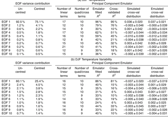
The emulator fittedR2 values are provided in Table 2. The PC1 emulator provides

5

a good fit to the simulator (R2_∼90 %). This has been found to be the case for all model outputs considered to date. The PC1 emulator is equivalent to an emulator of the global average change, scaling the first EOF to generate an emulation of the spa-tial distribution, so that high performance of the PC1 emulators is thus not surprising. Lower-order PC coefficients are generally harder to emulate, presumably because they

10

reflect physical processes that are more di_fficult to represent as simple functions of the input parameters and may contain increasing elements of internal variability. The emu-lator fits generally decrease fromR2_∼90 % (PC1) down to_∼30 % (PC10).

4.3 Cross-validation

A more robust measure of emulator performance is provided by cross-validated

statis-15

tics. Here, the emulator is built from the PC coefficients of the first 376 simulations and applied to estimate the PC coefficients for the remaining 188 simulations. The cross-validatedR2 values between emulated and actual PC coe_fficients are provided in Table 2. The performance of the PC1 emulator are not substantially degraded under cross-validation. However, lower order PC emulators, especially in the SAT variability

20

emulator, can perform quite poorly under cross-validation. In some instances, most extremely the PC4 emulator of DJF SAT variability (cross-validatedR2=6 %), the em-ulators serve little more than to add random noise. This demonstrates that the emu-lators cannot be assumed to provide a good approximation of the contribution of low order variability to an individual simulation. However, as the components are mutually

25

(16)

GMDD

6, 3349–3380, 2013

P. B. Holden et al.

Title Page

Tables Figures

◭ ◮

Back Close

Full Screen / Esc

Discussion

P

a

per

|

D

iscussion

P

a

per

|

Discussion

P

a

per

|

Discuss

ion

P

a

per

|

ensembles of PC coefficients have similar mean and standard deviation to the sim-ulated ensemble distributions. As the emsim-ulated fields are described by linear combi-nations of the EOFs, the necessary condition for the emulated ensemble to provide a good approximation to the simulated ensemble is that the ensemble distributions of the PC coefficients are well reproduced. We take this approach here, cross-validating

5

the statistics of the emulated ensemble. The PC1 emulators for both temperature and temperature variability reproduce the simulated ensemble distributions very well (Ta-ble 2). The emulated ensem(Ta-ble means for lower order EOFs also reproduce simulated ensemble means very well, although they somewhat understate the simulated ensem-ble standard deviation, by_∼19 % (temperature) and_∼27 % (temperature variability).

10

The lower order (2nd to 5th) PC SAT emulators were similarly found to underestimate the ensemble standard deviation by_∼20 % in Holden and Edwards (2010).

In summary, the emulated patterns of change are robust, but are subject to a rela-tively modest underestimate of the simulated ensemble variability. Robustness cannot be assumed for individual emulations although we note, given the high cross-validated

15

R2 of the PC1 emulators, that individual simulations are likely to be at least as well predicted as they would be under pattern scaling.

4.4 Spatio-temporal variability

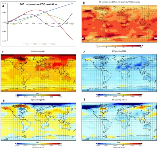
Figure 1a plots the temporal evolution of an illustrative subset of the EOFs of DJF tem-perature. For the purposes of this plot, each EOF is averaged over space at each time

20

slice (e.g. the average of elements 1 to 2048 describe the field at 2010). The first EOF describes an approximately linear temperature ramp. This EOF is the dominant mode of variability across the ensemble and so is expected to display an approximately linear increase over time because the 2nd and 3rd Chebyshev coe_fficients, which describe deviations from a linear ramp in CO2concentration, are both centred on zero in the

en-25

(17)

GMDD

6, 3349–3380, 2013

P. B. Holden et al.

Title Page

Tables Figures

◭ ◮

Back Close

Full Screen / Esc

Discussion

P

a

per

|

D

iscussion

P

a

per

|

Discussion

P

a

per

|

Discuss

ion

P

a

per

|

controlled by all three Chebyshev coefficients, the PC3 emulator is mainly controlled by TC2E and TC3E, and the PC10 emulator mainly by TC3E.

Figure 1b is a plot of the ratio of EOF1 at 2100 and 2010 time slices. This figure demonstrates that even when a single EOF is considered, the spatio-temporal emula-tion approach captures appreciable temporal evoluemula-tion of the spatial pattern. We note

5

that a pattern scaling approach would apply the same pattern at all times (i.e. equiva-lent to a uniform value everywhere in Fig. 1b). Figure 1c–f plot the spatial patterns at 2100 for each of the four EOFs illustrated in Fig. 1a. The second source of non-linear spatio-temporal variability thus arises from to the inclusion of the ten EOFs, which each exhibit distinct warming patterns. We do not attempt to ascribe physical meaning

10

to these patterns. It is well known that caution is required in interpreting EOF modes as physically based, although such an approach can be useful (Holden et al., 2013b). It is however worth noting that, as we apply the analysis to uncentred fields, the first EOF represents the ensemble averaged warming response, a pattern that is well known and robust across CMIP climate models (c.f. Figure 10.9, Meehl et al., 2007).

15

5 Baseline heating and cooling degree days

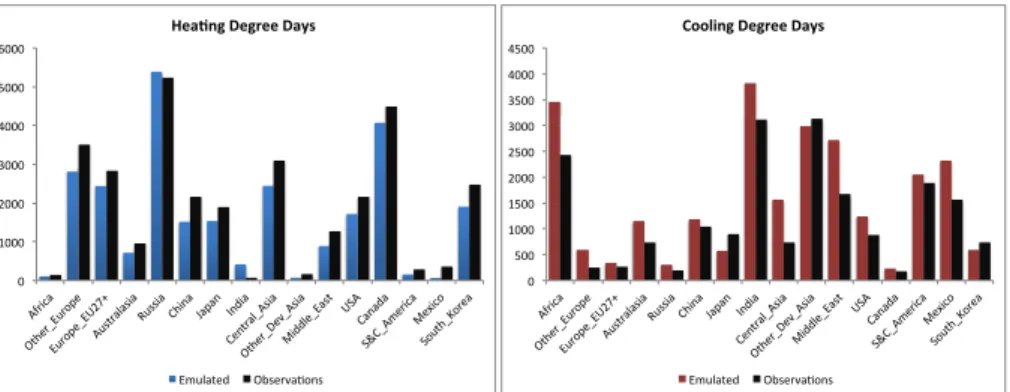
In this section we describe the derivation and validation of baseline (1 January 1995 to 1 January 2005) Heating Degree Days (HDDs) and Cooling Degree Days (CDDs), cal-culated on the PLASIM-ENTS grid and mapped onto the regions of the TIAM-WORLD model (TIMES integrated assessment model, Loulou and Labriet, 2008). HDDs provide

20

a measure that reflects heating energy demands, calculated relative to some baseline temperature. On a given day, the average temperature is calculated and subtracted from the baseline temperature. If the value is less than or equal to zero, then that day has zero HDDs (no heating requirements). If the value is positive, then that number represents the number of HDDs on that day. The sum of HDDs over a month

pro-25

(18)

GMDD

6, 3349–3380, 2013

P. B. Holden et al.

Title Page

Tables Figures

◭ ◮

Back Close

Full Screen / Esc

Discussion

P

a

per

|

D

iscussion

P

a

per

|

Discussion

P

a

per

|

Discuss

ion

P

a

per

|

a measure of the cooling demands for that month. An evaluation of the modern-day distribution of HDDs and CDDs therefore provides a useful validation of the baseline climate simulations, reflecting both spatial and seasonal variability, and furthermore provides a validation of the transformation of the emulated outputs into degree-day data and of the population-weighted mapping of this degree-day data onto the regional

5

level for impacts evaluation. The validation of the emulator itself will be addressed in Sect. 6.

We do not simulate (or emulate) degree-days directly but instead derive them from average seasonal temperature and daily variability, as defined by the standard devia-tion of the daily temperature across the season, following the approach of Schoenau

10

and Kehrig (1990). The critical assumption made is that daily temperatures are scat-tered about the monthly mean with a normal distribution. Direct calculation of degree-day data from daily variability would be more accurate, but was judged to be overly restrictive as it would prevent recalibration with an altered baseline temperature. Di_ff er-ent impact measures may apply different baselines, and baselines may be required to

15

change over time, or be defined differently from region to region. We calculate HDDs and CDDs at each PLASIM-ENTS grid cell from

HDD= N

σ√2π

B_H

Z

−∞

(BH−T)e

−(T₋µ)2/2σ2

dT (6)

CDD= N

σ√2π

∞

Z

B_C

(T₋BC)e

−(T−µ)2/2σ2

dT (7)

20

expressed in terms of the number of days in the seasonN, daily temperatureT, HDD baseline temperature BH, CDD baseline temperature BC, average daily temperature

(19)

GMDD

6, 3349–3380, 2013

P. B. Holden et al.

Title Page

Tables Figures

◭ ◮

Back Close

Full Screen / Esc

Discussion

P

a

per

|

D

iscussion

P

a

per

|

Discussion

P

a

per

|

Discuss

ion

P

a

per

|

BH=BC=18◦C is applied globally, although it is a straightforward modification to allow

the baselines to vary in space or over time.

For input to regionally integrated energy usage calculations in TIAM-WORLD, we derive a population-weighted average over the grid cells that comprise a given region. We apply 2005 population data (CIESIN and CIAT, 2005) at a 0.25◦resolution which we

5

integrate up onto the PLASIM-ENTS grid. We note that the low resolution of the climate model inevitably leads to approximations, most notably when highly populated regions near ocean are located in grid cells that are assigned to be ocean in PLASIM-ENTS. We address this here by assigning all grid cells that have a population greater than 500 000 to a TIAM-WORLD region, irrespective of whether or not that cell is assigned

10

to be land or ocean in PLASIM-ENTS. This avoids the potential neglect of densely populated coastal regions, but comes at the expense of ascribing an oceanic climate to some populated regions, likely understating seasonal variability and future warming. The seasonally resolved HDDs and CDDs are summed to generate annual data and are compared to observations (Baumert and Selman, 2003) in Fig. 2. PLASIM-ENTS

15

reproduces observational data remarkably well, capturing regional differences and with magnitudes that are generally quite reasonable. The emulator exhibits a warm bias, generally under-estimating HDDs and over-estimating CDDs. An element of this bias is likely due to recent warming as data sources for the observations are based on long-term averages that in the case of the United States for instance, includes data that

20

extends back to 1920.

6 Emulation of the Representative Concentration Pathways

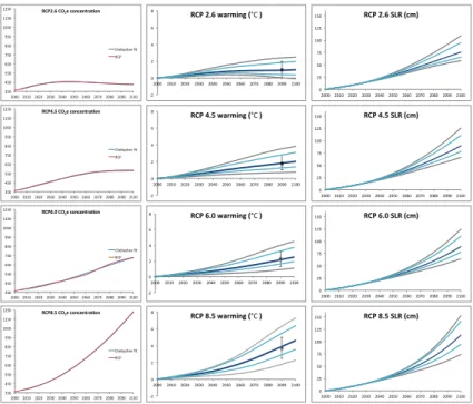
In order to evaluate the emulator, we consider the warming response to the forcing of the Representative Concentration Pathways RCPs (Moss et al., 2010). The four RCPs are consistent sets of projections of the components of future radiative forcing,

25

(20)

GMDD

6, 3349–3380, 2013

P. B. Holden et al.

Title Page

Tables Figures

◭ ◮

Back Close

Full Screen / Esc

Discussion

P

a

per

|

D

iscussion

P

a

per

|

Discussion

P

a

per

|

Discuss

ion

P

a

per

|

the precise RCP temporal profiles, but instead derive Chebyshev fitted pathways to each. These are illustrated in the first column of Fig. 3. In this validation we ascribe the same coefficients to both CO2e and CO2; CO2, is only an input to the vegetation in

PLASIM-ENTS and hence is of limited importance for temperature. These coefficients are then applied to the emulators of seasonal temperature to generate an ensemble of

5

188 warming fields, differing through their PLASIM-ENTS parameterisations.

The spatial patterns of emulated ensemble averaged DJF and June-July-August (JJA) warming over the future transient period (2100 to 2100 AD) are plotted in Fig. 4. These compare favourably to the patterns exhibited by CMIP3 AOGCMs (c.f. Fig. 10.9, Meehl et al., 2007). The largest differences are apparent in JJA warming. The

South-10

ern Ocean JJA warming is weaker than in the CMIP3 ensemble, likely a consequence of the fixed Antarctic sea ice in the training ensembles. South-east Asian JJA warming is also weaker in the emulator than in CMIP3 simulations, in fact displaying a cooling of up to_∼1.4 K under RCP4.5. This arises due to a strengthening of the South-east Asian monsoon in PLASIM-ENTS that is associated with decreased incoming

short-15

wave radiation (increased cloud cover) and increased evaporative cooling. Given the neglect of aerosol forcing in PLASIM-ENTS, this JJA cooling in south-east Asia should not be regarded as robust; aerosols are an important forcing of the south-east Asian monsoon through a range of likely competing effects (see e.g. Ganguly et al., 2012).

The temporal development of warming for each RCP is plotted in the second column

20

of Fig. 3. In all scenarios, the median ensemble warming compares favourably with the CMIP5 ensemble (Table 12.2, Collins et al., 2013). The emulated uncertainty is rep-resented by the 5th and 95th confidence intervals of the emulated ensemble, and is compared against the multi-model ranges of Collins et al. (2013). The emulator cap-tures the CMIP5 ranges well. The full range of the emulated ensemble is also plotted

25

to illustrate the emulated extremes.

(21)

GMDD

6, 3349–3380, 2013

P. B. Holden et al.

Title Page

Tables Figures

◭ ◮

Back Close

Full Screen / Esc

Discussion

P

a

per

|

D

iscussion

P

a

per

|

Discussion

P

a

per

|

Discuss

ion

P

a

per

|

assessment model (Bernard and Vielle, 2008). The sea level estimate is derived from the empirical form of Rahmstorf et al. (2012), which assumes that the rate of sea-level rise depends linearly on both warming and the rate of warming (Vermeer and Rahmstorf, 2009). We do not consider uncertainty in the empirical fit (estimated to be_∼ 10 % for RCP4.5) but instead apply the “CW05” fit throughout. We note that the median

5

emulated sea level prediction for RCP4.5 (89 cm) is slightly lower than the Rahmstorf et al. (2012) estimate (_∼1 m), despite a slightly greater 2100–2000 AD warming (2.0 K compared to 1.8 K). This may reflect a somewhat greater thermal inertia in the PLASIM-ENTS ensemble, as also evidenced by the emulated warming under RCP 2.6, which continues to warm through the 21st Century in the emulated ensemble median despite

10

the decreasing radiative forcing after 2040 AD.

7 Conclusions

Building on Holden and Edwards (2010), we have developed an emulator of the spatio-temporal climate response to an arbitrary 21st Century forcing scenario. We apply sin-gular vector decomposition to decompose the modes of variability across a large

en-15

semble of simulations of the intermediate complexity GCM PLASIM-ENTS. We emulate the high-order principal components as simple polynomial functions of future forcing and model parameters that we apply to emulate fields of climate change in response to an arbitrary forcing profile. The approach represents an advance on pattern scaling as it allows us to address non-linear spatio-temporal feedbacks and uncertainty.

20

The motivation for this approach is computational speed. A 188-member ensemble of 100 yr PLASIM-ENTS simulations requires_∼1 CPU year. A 188-member emulated ensemble requires_∼1 CPU second per output variable.

The approach does not quantify emulator error (or “code uncertainty”). However, we do evaluate the error that arises from parametric uncertainty. We demonstrate under

25

(22)

GMDD

6, 3349–3380, 2013

P. B. Holden et al.

Title Page

Tables Figures

◭ ◮

Back Close

Full Screen / Esc

Discussion

P

a

per

|

D

iscussion

P

a

per

|

Discussion

P

a

per

|

Discuss

ion

P

a

per

|

simulated ensemble by_∼20 %. In essence, the approach provides a robust emulation (the emulated mean) of the simulator response to the control variables (describing the future forcing), together with an evaluation of the cloud of uncertainty that is derived from the emulated parametric uncertainty.

The emulator reproduces present-day regionally resolved heating and cooling days

5

that are in good agreement with observations. It generates spatial patterns and tempo-ral profiles of seasonally resolved warming and associated uncertainty that are in gen-erally good agreement with the CMIP ensemble of atmosphere–ocean GCMs, making it an appropriate tool for impact assessment. Although not described here, we note that we have also applied the approach to emulate precipitation, evaporation and

frac-10

tional cloud cover for application to energy demands (hydroelectric potential) and crop impacts. These will be discussed in future work.

Acknowledgements. This work was funded under EU FP7 ERMITAGE grant no. 265170.

References

Annan, J. D., Lunt, D. J., Hargreaves, J. C., and Valdes, P. J.: Parameter estimation in an

15

atmospheric GCM using the Ensemble Kalman Filter, Nonlin. Processes Geophys., 12, 363– 371, doi:10.5194/npg-12-363-2005, 2005.

Bordi, I., Fraedrich, K., Sutera, A., and Zhu, X.: Transient response to well-mixed green-house gas changes, Theor. Appl. Climatol., 109, 245–252, doi:10.1007/s00704-011-0580-z, 2011a.

20

Bordi, I., Fraedrich, K., Sutera, A., and Zhu, X.: On the climate response to zero ozone, Theor. Appl. Climatol., 109, 253–259, doi:10.1007/s00704-011-0579-5, 2011b.

Bordi, I., Fraedrich, K., Sutera, A., and X. Zhu, X.: On the effect of decreasing CO₂ concen-trations in the atmosphere, Clim. Dynam., 40, 651–662, doi:10.1007/s00382-012-1581-z, 2013.

25

(23)

GMDD

6, 3349–3380, 2013

P. B. Holden et al.

Title Page

Tables Figures

◭ ◮

Back Close

Full Screen / Esc

Discussion

P

a

per

|

D

iscussion

P

a

per

|

Discussion

P

a

per

|

Discuss

ion

P

a

per

|

CIESIN and CIAT (Center for International Earth Science Information Network and Columbia University; and Centro Internacional de Agricultura Tropical): Gridded Population of the World, Version 3 (GPWv3), Socioeconomic Data and Applications Center (SEDAC), Columbia University, Palisades, NY, available at: http://sedac.ciesin.columbia.edu/gpw, downloaded 20 March 12, 19 June 2013, 2005.

5

Collins, M., Knutti, R., Arblaster, J., Dufresne, J.-L., Fichefet, T., Friedlingstein, P., Gao, X., Gutowski, W., Johns, T., Krinner, G., Shongwe, M., Tebaldi, C., Weaver, A., and Wehner, M.: Long-term climate change: projections, commitments and irreversibility, in: Climate Change 2013: The Physical Science Basis, Contribution of WG I to the Fifth Assessment Report of the IPCC, edited by: Stocker, T. and Qin, D., Cambridge University Press, Cambridge, UK

10

and New York, USA, in preparation, 2013.

Conti, S. and O’Hagan, A.: Bayesian emulation of complex multi-output and dynamic computer models, J. Stat. Plan. Infer., 140, 640–651, doi:10.1016/j.jspi.2009.08.006, 2010.

Dekker, S. C., de Boer, H. J., Brovkin, V., Fraedrich, K., Wassen, M. J., and Rietkerk, M.: Biogeo-physical f eedbacks trigger shifts in the modelled vegetation-atmosphere system at multiple

15

scales, Biogeosciences, 7, 1237–1245, doi:10.5194/bg-7-1237-2010, 2010.

Edwards, N. R., Cameron, D., and Rougier, J.: Precalibrating an intermediate complexity cli-mate model, Clim. Dynam., 37, 1469–1482, doi:10.1007/s00382-010-0921-0, 2011.

Fraedrich, K.: A suite of user-friendly global climate models: hysteresis experiments, Eur. Phys. J. Plus, 127, 53, doi:10.1140/epjp/i2012-12053-7, 2012.

20

Fraedrich, K. and Lunkeit, F.: Diagnosing the entropy budget of a climate model, Tellus A, 60, 921–931, doi:10.1111/j.1600-0870.2008.00338.x, 2008.

Fraedrich, K., Jansen, H., Kirk, E., Luksch, U., and Lunkeit, F.: The Planet Simulator: towards a user friendly model, Meteorol. Z., 14, 299–304, doi:10.1127/0941-2948/2005/0043, 2005a. Fraedrich, K., Kirk, E., Luksch, U., and Lunkeit, F.: The portable university model of the

atmo-25

sphere (PUMA): storm track dynamics and low-frequency variability, Meteorol. Z., 14, 735– 745, doi:10.1127/0941-2948/2005/0074, 2005b.

Ganguly, D., Rasch, P. J., Wang, H., and Yoon, J.-H.: Climate response of the South Asian monsoon system to anthropogenic aerosols, J. Geophys. Res., 117, D13209, doi:10.1029/2012JD017508, 2012.

30

(24)

GMDD

6, 3349–3380, 2013

P. B. Holden et al.

Title Page

Tables Figures

◭ ◮

Back Close

Full Screen / Esc

Discussion

P

a

per

|

D

iscussion

P

a

per

|

Discussion

P

a

per

|

Discuss

ion

P

a

per

|

Holden, P. B. and Edwards, N. R.: Dimensionally reduced emulation of an AOGCM for application to integrated assessment modelling, Geophys. Res. Lett., 37, L21707, doi:10.1029/2010GL045137, 2010.

Holden, P. B., Edwards, N. R., Oliver, K. I. C., Lenton, T. M., and Wilkinson, R. D.: A probabilistic calibration of climate sensitivity and terrestrial carbon change in GENIE-1, Clim. Dynam., 35,

5

785–806, doi:10.1007/s00382-009-0630-8, 2010.

Holden, P. B., Edwards, N. R., Gerten, D., and Schaphoff, S.: A model-based constraint on CO₂ fertilisation, Biogeosciences, 10, 339–355, doi:10.5194/bg-10-339-2013, 2013a.

Holden, P. B., Edwards, N. R., Müller, S. A., Oliver, K. I. C., Death, R. M., and Ridgwell, A.: Controls on the spatial distribution of oceanic δ13CDIC, Biogeosciences, 10, 1815–1833,

10

doi:10.5194/bg-10-1815-2013, 2013b.

Lenton, T. M., Aksenov, Y., Cox, S. J., Hargreaves, J. C., Marsh, R., Price, A. R., Lunt, D. J., An-nan, J. D., Cooper-Chadwick, T., Edwards, N. R., S. Goswami, S., Livina, V. N., Valdes, P. J., Yool, A., Harris, P. P., Jiao, Z., Payne, A. J., Rutt, I. C., Shepherd, J. G., Williams, G., and Williamson, M. S.: Effects of atmospheric dynamics and ocean resolution on bistability of the

15

thermohaline circulation examined using the Grid Enabled Integrated Earth system modelling (GENIE) framework, Clim. Dynam., 29, 591–613, doi:10.1007/s00382-007-0254-9, 2007. Lucarini, V., Fraedrich, K., and Lunkeit, F.: Thermodynamic analysis of snowball earth

hystere-sis experiment: efficiency, entropy production, and irreversibility, Q. J. Roy. Meteor. Soc., 136, 2–11, doi:10.1002/qj.543, 2010.

20

Matthews, H. D., Eby, M., Ewen, T., Friedlingstein, P., and Hawkins, B. J.: What determines the magnitude of carbon cycle-climate feedbacks?, Global Biogeochem. Cy., 21, GB2012, doi:10.1029/2006GB002733, 2007.

Meehl, G. A., Stocker, T. F., Collins, W. D., Friedlingstein, P., Gaye, A. T., Gregory, J. M., Ki-toh, A., Knutti, R., Murphy, J. M., Noda, A., Raper, S. C. B., Watterson, I. G., Weaver, A. J.,

25

and Zhao, Z.-C.: Global climate projections, in: Climate Change 2007: The Physical Science Basis, Contribution of Working Group I to the Fourth Assessment Report of the Intergovern-mental Panel on Climate Change, edited by: Solomon, S., Qin, D., Manning, M., Chen, Z., Marquis, M., Averyt, K. B., Tignor, M., and Miller, H. L., Cambridge University Press, Cam-bridge, UK and New York, NY, USA, 2007.

30

(25)

GMDD

6, 3349–3380, 2013

P. B. Holden et al.

Title Page

Tables Figures

◭ ◮

Back Close

Full Screen / Esc

Discussion

P

a

per

|

D

iscussion

P

a

per

|

Discussion

P

a

per

|

Discuss

ion

P

a

per

|

Micheels, A. and Montenari, M.: A snowball Earth versus a slushball Earth: results from Neo-proterozoic climate modeling sensitivity experiments, Geosphere, 4, 401–410, 2008. Mitchell, J. F. B., Johns, T. C., Eagles, M., Ingram, W. J., and Davis, R. A.:

To-wards the construction of climate change scenarios, Climatic Change, 41, 547–581, doi:10.1023/A:1005466909820, 1999.

5

Moss, R. H., Edmonds, J. A., Hibbard, K. A., Manning, M. R., Rose, S. K., van Vuuren, D. P., Carter, T. R., Emore, S., Kainuma, M., Kram, T., Meehl, G. A., Mitchell, J. F. B., Naki-cenovic, N., Riahi, K., Smith, S. J., Stouffer, R. J., Thompson, A. M., Weyant, J. P., and Wilbanks, T. J.: The next generation of scenarios for climate change research and assess-ment, Nature, 463, 747–756, doi:10.1038/nature08823, 2010.

10

O’Hagan, A.: Bayesian analysis of computer code outputs: a tutorial, Reliab. Eng. Syst. Safe., 91, 1290–1300, doi:10.1016/j.ress.2005.11.025, 2006.

R Development Core Team: R: a Language and Environment for Statistical Computing, R Foun-dation for Statistical Computing, Vienna, Austria, available at: http://www.R-project.org, (19 June 2013), 2013.

15

Ramhstorf, S., Perrette, M., and Vermeer, M.: Testing the robustness of semi-empirical sea level projections, Clim. Dynam., 39, 861–875, doi:10.1007/s00382-011-1226-7, 2012.

Roscher, M., Stordal, F., and Svensen, H.: The effect of global warming and global cooling on the distribution of the latest Permian climate zones, Palaeogeogr. Palaeocl., 309, 186–200, doi:10.1016/j.palaeo.2011.05.042, 2011.

20

Schmittner, A., Silva, T. A. M., Fraedrich, K., Kirk, E., and Lunkeit, F.: Effects of mountains and ice sheets on global ocean circulation, J. Climate, 24, 2814–2829, doi:10.1175/2010JCLI3982.1, 2011.

Santner, T. J., Williams, B. J., and Notz, W. I.: The Design and Analysis of Computer Experi-ments, Springer, New York, 2003.

25

Schoenau, G. J. and Kehrig, R. A.: A method for calculating degree-days to any base temper-ature, Energ. Buildings, 14, 299–302, doi:10.1016/0378-7788(90)90092-W, 1990.

Stenzel, O., Grieger, B., Keller, H. U., Greve, R., Fraedrich, K., and Lunkeit, F.: Coupling Planet Simulator Mars, a general circulation model of the Martian atmosphere, to the ice sheet model SICOPOLIS, Planet. Space Sci., 55, 2087–2096, doi:10.1016/j.pss.2007.09.001,

30

2007.

(26)

GMDD

6, 3349–3380, 2013

P. B. Holden et al.

Title Page

Tables Figures

◭ ◮

Back Close

Full Screen / Esc

Discussion

P

a

per

|

D

iscussion

P

a

per

|

Discussion

P

a

per

|

Discuss

ion

P

a

per

|

Vermeer, M. and Rahmstorf, S.: Global sea level linked to global temperature, P. Natl. Acad. Sci. USA, 106, 21527–21532, doi:10.1073/pnas.0907765106, 2009.

Wilkinson, R. D.: Bayesian calibration of expensive multivariate computer experiments, in: Large Scale Inverse Problems and the Quantification of Uncertainty, Wiley Series in Com-putational Statistics, edited by: Biegler, L. T., Biros, G., Ghattas, O., Heinkenschloss, M.,

5

Keyes, D., Mallick, B. K., Tenorio, L., Van Bloemen Waanders, B., and Wilcox, K., John Wiley and Sons Ltd, Chichester, UK, 2011.

Williamson, M. S., Lenton, T. M., Shepherd, J. G., and Edwards, N. R.: An efficient numer-ical terrestrial scheme (ENTS) for Earth system modelling, Ecol. Model., 198, 362–374, doi:10.1016/j.ecolmodel.2006.05.027, 2006.

(27)

GMDD

6, 3349–3380, 2013

P. B. Holden et al.

Title Page

Tables Figures

◭ ◮

Back Close

Full Screen / Esc

Discussion

P

a

per

|

D

iscussion

P

a

per

|

Discussion

P

a

per

|

Discuss

ion

P

a

per

|

Table 1.The twenty-two parameters and their prior ranges.

Module Parameter Process Min Max Units

PUMA vdiff_lamm Vertical diffusivity 10 500 m

PUMA nhdiff Cut-offwavenumber for horizontal diffusivity 14 16

PUMA tdissd Horizontal di_ffusivity of divergence 0.05 10 days

PUMA tdissz Horizontal diffusivity of vorticity 0.05 10 days

PUMA tdisst Horizontal diffusivity of temperature 0.05 10 days

PUMA tdissq Horizontal diffusivity of moisture 0.05 10 days

PLASIM rhcritmin Minimum relative critical humidity 0.5 1.0

PLASIM gamma Evaporation of precipitation 0.001 0.05

PLASIM tswr1 SW clouds (visible) 0.01 0.5

PLASIM tswr2 SW clouds (infra red) 0.01 0.5

PLASIM acllwr LW clouds 0.01 5.0 m−2g−1

PLASIM th20c LW water vapour 0.01 0.1

SEA ICE xmind Minimum sea-ice thickness 0.10 0.3 m

OCEAN albseamax Ocean albedo (αsEq. 2) 0.10 0.3

OCEAN dlayer Ocean slab thickness 300 700 m

ENTS k14 Photosynthesis CO2 fertilisation 30 750 ppm

ENTS tadj Photosynthesis optimum temperature adjustment 0.0 5.0 K

ENTS qthresh Photosynthesis moisture threshold 0.10 0.5

ENTS k17 Fractional vegetation dependence 0.25 1.0 kg C m−2

ENTS k18 Base photosynthesis rate 3.0 7.0 kg C m−2yr−1

ENTS k26 Leaf litter rate 0.075 0.26 yr−1

(28)

GMDD

6, 3349–3380, 2013

P. B. Holden et al.

Title Page

Tables Figures

◭ ◮

Back Close

Full Screen / Esc

Discussion

P

a

per

|

D

iscussion

P

a

per

|

Discussion

P

a

per

|

Discuss

ion

P

a

per

|

Table 2.Summary description and validation of the (a) DJF temperature and (b) DJF

tempera-ture variability emulators.

(a) DJF Temperature

EOF variance contribution Principal Component Emulator

Un- Centred Number of Number of Emulator Cross- Simulated Emulated centred linear quad/cross fitted validated cross-val cross-val terms terms R2 R2 distribution distribution EOF 1 92.5 % 75.1 % 17 10 96 % 95 % 0.036±0.020 0.037±0.021 EOF 2 1.2 % 4.1 % 12 10 79 % 76 % −0.003±0.046 −0.000±0.039 EOF 3 0.6 % 2.2 % 14 9 30 % 10 % 0.001±0.042 −0.003±0.024 EOF 4 0.5 % 1.8 % 17 10 62 % 51 % −0.007±0.044 −0.005±0.034 EOF 5 0.4 % 1.1 % 16 10 59 % 45 % −0.010±0.039 −0.012±0.032 EOF 6 0.2 % 0.8 % 12 8 42 % 21 % −0.004±0.038 −0.003±0.031 EOF 7 0.2 % 0.7 % 15 10 45 % 32 % 0.003±0.042 0.005±0.028 EOF 8 0.2 % 0.6 % 21 10 41 % 19 % −0.004±0.041 −0.002±0.030 EOF 9 0.2 % 0.6 % 12 9 30 % 18 % 0.001±0.042 −0.001±0.026 EOF 10 0.1 % 0.5 % 15 9 36 % 9 % −0.002±0.039 −0.002±0.031

(b) DJF Temperature Variability

EOF variance contribution Principal Component Emulator

Un- Centred Number of Number of Emulator Cross- Simulated Emulated centred linear quad/cross fitted validated cross-val cross-val

terms terms R2 _R2