Abstract
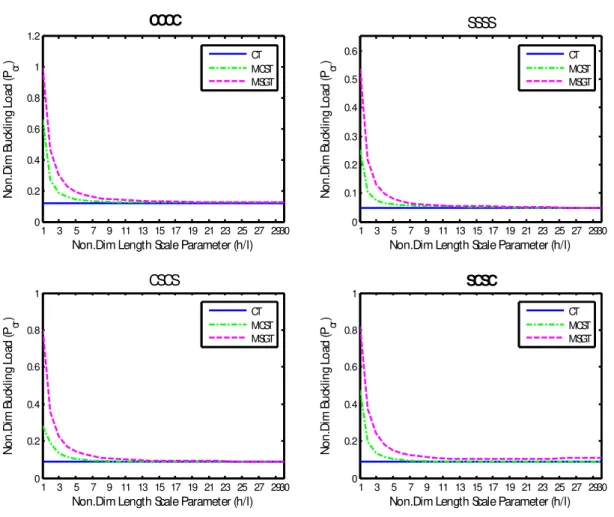
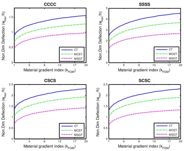
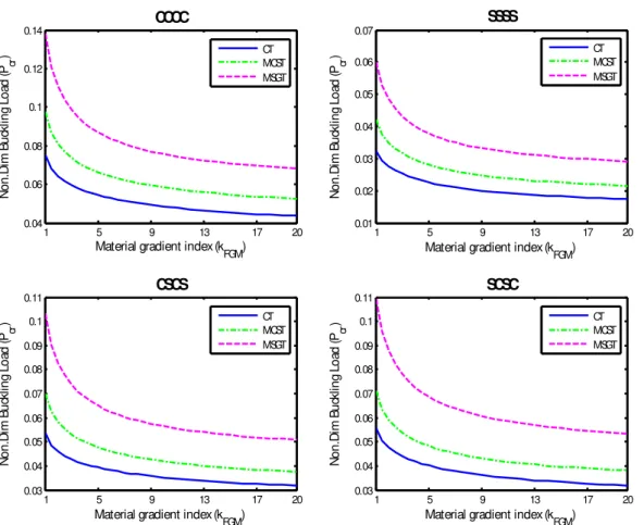
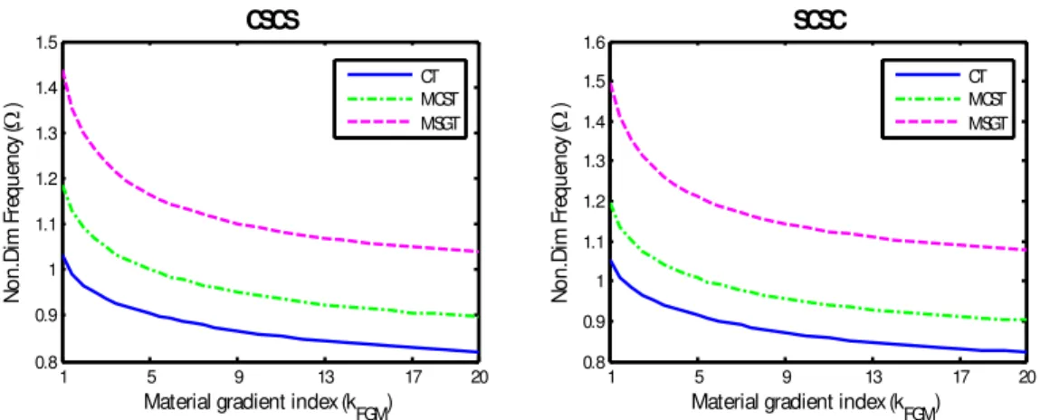
In this paper, a size-dependent microscale plate model is developed to describe the bending, buckling and free vibration behaviors of microplates made of functionally graded materials (FGMs). The size effects are captured based on the modified strain gradient theory (MSGT), and the formulation of the paper is on the basis of Mindlin plate theory. The presented model accommodates the models based upon the classical theory (CT) and the modified couple stress theory (MCST) if all or two scale parameters are set to zero, respectively. By using Hamilton’s principle, the governing equations and related boundary conditions are derived. The bending, buckling and free vibration problems are considered and are solved through the generalized differential quadrature (GDQ) method. A detailed parametric and comparative study is conducted to evaluate the effects of length scale parameter, material gradient index and aspect ratio predicted by the CT, MCST and MSGT on the deflection, critical buckling load and first natural frequency of the microplate. The numerical results indicate that the model developed herein is significantly size-dependent when the thickness of the microplate is on the order of the material scale parameters.
Keywords
Bending; Buckling; Free vibration; FGM microplate; Strain gradient theory; GDQ.
Size-Dependent Bending, Buckling and Free Vibration Analyses of
Microscale Functionally Graded Mindlin Plates Based on the Strain
Gradient Elasticity Theory
1 INTRODUCTION
The experiments conducted on the microstructures subjected to different loading conditions have revealed their size–dependent behavior (Nix 1989; Fleck et al. 1994; Ma and Clarke 1995; Vardoulakis et al. 1998; Stolken and Evans 1998; Chong and Lam 1999; Lam et al. 2003; and Colton 2005). When the dimensions of a structure are on the order of microns or submicrons, it
R. Ansari a E. Hasrati a M. Faghih Shojaei a R. Gholami b V. Mohammadi a A. Shahabodini a
a Department of Mechanical Engineering
University of Guilan, Rasht, Iran, P.O. Box 41635-3756
b Department of Mechanical Engineering
Lahijan Branch, Islamic Azad
University, Lahijan, Iran, P.O. Box 1616
* Corresponding author; Tel. /fax: +98 131 6690276. E-mail address:
http://dx.doi.org/10.1590/1679-78252322
is necessary to consider internal material length scale parameters in order to predict its mechanical behavior. Conducting experiments on the microstructures is difficult and with high expenses. Hence, the continuum mechanics has attracted the attention of researchers for the modeling of microstructures. The classical continuum theories are not proper for identifying the behavior of small scale structures, because in such theories the character of stress is local with no material length scale. This shortcoming in the conventional continuum mechanics motivated some researchers to develop the non-classical theories taking the size effects into account.
One of the most significant higher-order continuum theories presented by Mindlin (1965) is gradient theory in which the first and second derivatives of the strain tensor effective on the strain energy density are included. Further, Fleck and Hutchinson (1993) extended Mindlin’s theory and proposed the strain gradient theory which involves five material constants in the constitutive equations. In this theory, higher order stress components are appeared due to the stretch and rotation gradient tensors. Also, Toupin (1964), Mindlin and Tiersten (1962) used a higher order theory and developed the classical couple stress theory which included two material parameters. Determination of the material constants is one of the challenges these theories face. That’s why; the works were done toward the modification of the mentioned theories and consequently, the reduction of the number of the length scale parameters involved. In this direction, the modified couple stress theory (MCST) was initiated by Yang et al (2002) in which only one length scale parameter is used in the constitutive equations leading to the symmetric couple stress tensor. Relevant works concerning the applicability of MCST in the analysis of microstructures can be found in (Ma et al. (2008); Tsiatas (2009); Kahrobaiyan et al. (2010); Ke et al. (2011); Jomehzadeh et al. (2011); Asghari (2012); Thai and Choi (2013)). In addition to these works, based on the modified couple stress and Kirchhoff plate theories, a size-dependent plate model was developed by Yin et al. (2010) for the dynamic analysis of microplate. Nateghi et al. (2012) employed the MCST and three different beam theories, i.e. classical, first and third order shear deformation beam theories to study the size effects on buckling load of functionally graded microbeams. Ke et al. (2012) studied the free vibrations of microplates on the basis of the modified couple stress and Mindlin plate theories.
Altan and Aifantis (1992) suggested a simplified strain gradient model including a single strain gradient coefficient of length squared dimension. Based on this model, Lazopoulos (2004) investigated the buckling behavior of a long rectangular plate subjected to uniaxial compression and small lateral load.
Lam et al. (2003) reduced five scale constants in strain gradient theory to three ones and presented the modified strain gradient theory. The constant are associated with dilatation gradient, deviatoric gradient and symmetric rotation gradient tensors so, this theory contains several higher-order stress components compared to the MCST.
al. (2011) did the static bending, instability and free vibration problems of an all edges simply supported rectangular micro-plate based on a size-dependent Kirchhoff micro-plate model. A comprehensive geometrically nonlinear size-dependent Timoshenko beam model was developed by Ansari et al. (2012) based on strain gradient and von Kármán theories. They applied the model and described the nonlinear free vibration of simply supported microbeam. Kahrobian et al. (2012) proposed a non-classical beam model accounting for the size influences in the framework of Euler– Bernoulli beam and strain gradient theories for static and free vibrations analyzes. They derived five equivalent length scale parameters in terms of the length scales of material constituents for functionally graded microbeams. Ansari et al. (2013) analyzed the pull-in instability of circular microplates based on the Kirchhoff plate theory and MSGT.
The novel thermo-mechanical properties of FGM make them as a prime candidate to be used in a wide range of engineering applications. These materials are also employed in the micro and nano-sized structures such as micro and nano–electromechanical systems and atomic force microscopes. Thus, to have a proper design of these systems, the knowledge of the mechanical behavior of FG microstructures is necessary. Recently, some research works have been conducted on the microscale structure made of functionally grade materials (Sahmani and Ansari (2013); Asghari et al. (2011); Ansari et al. (2011)).
In this paper, a non-classical size-dependent plate model is developed for the bending, buckling and free vibration analyses of microscale FG plates. The model takes the important size influences and the effect of transverse shear deformation into account through incorporating the strain gradient elasticity theory into the Mindlin plate theory. The constitutive relations of the present model have three length scale parameters, and for some specific values of the length scale material parameters, this model can be reduced to that based on the modified couple stress theory. Furthermore, the proposed model considers the influences of thermal environments on the static and dynamic responses of the FG microplates. Hamilton’s principle is utilized to derive the governing equations and corresponding boundary conditions. Also the current solution algorithm is based on the generalized differential quadrature (GDQ) method which enables one to impose any arbitrary boundary condition. So, in this work, the behavior of FG microscale plates with various edge conditions is studied. In the numerical results, the effects of different model parameters on the response of the microplate are investigated.
2 SIZE-DEPENDENT GOVERNING EQUATIONS AND BOUNDARY CONDITIONS
2.1 Modeling the Material Properties of FG Microplate
Figure 1: Schematic of an FG microplate under bi-axial loading and uniformly distributed transverse load: coordinate system and geometric parameters.
In the present work, the material properties of FGM, Young’s modulus
E
, Poisson’s ratio
, mass density
, thermal conductivityK
and thermal expansion coefficient
are taken to be of the following form
,
,
,
c c m m c c m m c c m m
c c m m c c m m
E z
E V
E V
z
V
V
z
V
V
z
V
V
K z
K V
K V
(1)The volume fractions of ceramic and of metal,
V
c andV
m respectively, are assumed to follow apower function of a spatial variable as
1
z
,
1
2
h
FGM k
c m c
V
z
V
V
(2)where
k
FGM is the volume fraction or material gradient exponent. It is obvious that as the value ofFGM
k
approaches infinity the plate becomes fully metal and as it tends to zero the plate reduces to a fully ceramic one.2.2 Kinematics of Microplate
in-plane displacements are stated as linear functions of the plate thickness and the transverse deflection is considered to be constant along the plate thickness causing the displacement field to be expressed as
1
, ,
x, ,
,
2, ,
y, ,
,
3, ,
.
u
u t x y
z
t x y
u
v t x y
z
t x y
u
w t x y
(3)2.3 Constitutive Equations Based on the Modified Strain Gradient Theory
In comparison with the modified couple stress theory, the strain gradient theory proposed by Lam et al. (2003) includes two additional gradient tensors namely the dilatation gradient tensor and the deviatoric stretch gradient tensor. Assuming infinitesimal deformations, the strain energy
Π
s stored in a continuum elastic medium occupying regionΩ
is expressed as
(1) (1)
s
Ω
1
Π
Ω
2
s s
ij ij
p
i i ijk ijkm
ij ijd
(4)where
ij, ,
i ijk(1),
ijs ( , ,i j k x, y, z) denote the components of the strain tensor, the dilatation gradient tensor, the deviatoric stretch gradient tensor and the symmetric rotation gradient tensor, respectively given by
, ,
1
2
ij
u
i ju
j i
(5-1),
i mm i
(5-2)
(1)
, , ,
1
1
;
,
3
3
s s s s s
ijk ijk ij mmk jk mmi ki mmj ijk jk i ki j ij k
(5-3)
, ,
1
;
2
s
ij i j j i
(5-4)
1
2
i
curl u
i
(5-5)in which
u
i,
i represent the components of the displacement vectoru
and the infinitesimal rotation vector
, respectively and the symbol
denotes the Kronecker delta. The classical stress tensor
ij and the higher–order stresses(1)
,
,
si ijk ij
p
m
corresponding to a linear isotropic elastic material are stated as
2 (1) 2 (1) 20 1 2
2
,
2
,
2
,
s2
sij
tr
ij ijp
il
i ijkl
ijkm
ijl
ij
(6)0
Furthermore, the parameters 2
1
E
and 2(1 )
E
stand for the bulk and shear modules,
respectively.
By substitution of Eqs. (3) into Eq. (5-5), one can get the components of infinitesimal rotation vector as
1
1
1
,
,
.
2
2
2
2
y x
x y y x z
w
w
v
u
z
y
x
x
y
y
x
(7)The nonzero components of the strain–displacement relations can be obtained by introducing Eq. (3) into Eq. (5-1), as
1
,
,
,
2
2
1
1
,
.
2
2
y y
x x
xx yy xy
xz x yz y
u
v
u
v
z
z
z
x
x
y
y
y
x
y
x
w
w
x
y
(8)
The components of other three gradient tensors i.e.,
γ χ
, ,
are derived by introducing Eqs. (7) and (8) into Eqs. (5-2)-(5-4) as:The dilatation gradient tensor:
2 2
2 2
2 2 2 2
2 2
,
2 2,
.
y y y
x x x
x y z
u
v
v
u
z
z
x
x y
x
x y
y
x y
y
x y
x
y
(9)The deviatoric stretch gradient tensor:
1 2 2 2 2 2 2
2 2 2 2
1
2
2
2
2
,
5
5
y
x x
xxx
u
u
v
z
x
y
x y
x
y
x y
1 2 2 2 2 2 2
2 2 2 2
1
2
2
2
2
,
5
5
y y x
yyy
v
v
u
z
y
x
x y
y
x
x y
2 2
(1)
2 2
2
1
,
5
5
y x
zzz
w
w
x
y
x
y
2 2
2
2 2 2
(1) (1) (1)
2 2 2 2
1
4
8
3
8
4
3
,
15
15
y y
x
xxy xyx yxx
v
u
v
z
x
x y
y
x y
x
y
2 2
(1) (1) (1)
2 2
1
4
8
2
,
15
y x
xxz xzx zxx
w
w
x
y
x
y
2 2 2
2 2 2
(1) (1) (1)
2 2 2 2
1
4
3
8
8
4
3
,
15
15
y y x
yyx yxy xyy
u
u
v
z
y
x
x y
x y
y
x
2 2 (1) (1) (1)
2 2
1
4
2
8
,
15
y x
yyz yzy zyy
w
w
y
x
x
y
2
2 2
2 2 2
(1) (1) (1)
2 2 2 2
1
3
2
3
2
,
15
15
y
x x
zzx zxz xzz
u
v
u
z
x
x y
y
x
x y
y
2 2 2
2 2 2
(1) (1) (1)
2 2 2 2
1
3
2
3
2
,
15
15
y y x
zzy zyz yzz
v
v
u
z
x
y
x y
x
y
x y
2 (1) (1) (1) (1) (1) (1)
1
3
y x
xyz yzx zxy xzy yxz zyx
w
x y
y
x
The symmetric rotation gradient tensor:
2 2
1
1
1
,
,
,
2
2
2
y y
s s x s x
xx yy zz
w
w
x y
x
x y
y
y
x
2 2
2 2 2 2
2 2 2 2
1
1
,
,
4
4
4
y y
s x s x
xy xz
w
w
v
u
z
y
x
y
x
x
x y
x y
x
2 2
2 2
2 2
1
.
4
4
y
s x
yz
v
u
z
x y
y
y
x y
(11)
On substitution of Eqs. (8)-(11) into (6), the constitutive equations corresponding to the classical and strain gradient theories are obtained.
2.4 Derivation of General Form of Governing Equations and Boundary Conditions
The microplate is first considered to be subjected to the in-plane prebuckling forces
N
xx0 ,0
yy
N
and0
xy
N
and the transverse load q t x y( , , ) as shown in Fig. 1. Herein, to derive the equations ofmotion, Hamilton’s principle is employed which is expressed as follows
2
1
0,
t
T s w
t
dt
(12)where
T and
w are the kinetic energy of FG microplate and the work done by the externalloads, respectively. From Eq. (4), the total strain energy can be written as the addition of strain energies corresponding to the classical stresses
C, the dilatation stresses
NC1, the deviatoric stretch stresses
NC2 and the couple stresses
NC3 as1 2 3
S C NC NC NC
The normal resultant forces, shear forces, bending moments and couple moments are related to the components of classical and the couple stress tensors as follows
/ 2/ 2
,
,
,
,
(
,
,
,
,
)
,
h
xx yy xy x y xx yy xy s xz s yz
h
N
N
N
Q Q
k
k
dz
(14-1)
/ 2
/ 2
,
,
,
,
,
h
xx yy xy xx yy xy
h
M
M
M
zdz
(14-2)
/ 2
/ 2
,
,
,
,
,
,
,
,
,
,
,
h
s s s s s s
xx yy zz xy xz yz xx yy zz xy xz yz
h
Y
Y
Y Y
Y Y
m
m
m
m
m
m
dz
(14-3)
/ 2
/ 2
,
,
,
h
s s
xz yz xz yz
h
H
H
m
m
zdz
(14-4)where
k
s denotes the shear correction factor.The effective higher order stresses on a section defined above lead to the higher-order resultants force and moments in the section which are stated as
/ 2
x
/ 2
,
,
,
,
h
y z x y z
h
P P P
p p
p
dz
(15-1)
/ 2
1 1 1 1 1 1 1 1
/ 2,
,
,
,
,
,
,
,
,
,
,
,
,
,
h
xxx yyy zzz xxy xxz yyx yyz xyz xxx yyy zzz xxy xxz yyx yyz xyz
h
T
T
T
T
T
T
T
T
dz
(15-2)
/ 2
/ 2
1 1 1 1
/ 2 / 2
,
,
,
,
,
,
,
,
,
h h
p p
x y x y xxx yyy xxy yyx xxx yyy xxy yyx
h h
M
M
p p
zdz M
M
M
M
zdz
(15-3)The strain energies associated with the classical elastic theory and strain gradient theory appeared in Eq. (13) can be obtained by using Eqs. (14) and (15) as
Ω
1
1
Ω
2
2
,
y x
C ij ij xx xx yy yy xy
A
y x
xy x x y y
u
v
u
v
d
N
M
N
M
N
x
x
y
y
y
x
w
w
M
Q
Q
dA
y
x
x
y
2 2
2 2 2 2
1 x 2 2 y 2
Ω 2 2 z 2
1
1
Ω
2
2
,
y p xNC i i x
A
y y
p x x
y
u
v
v
u
p
d
P
M
P
x
x y
x
x y
y
x y
M
P
dA
y
x y
x
y
(16-2) 1 1 2 2 2 2 2
2 2 2 2 2
Ω
2 2 2 2
2 2
2
2
1 1
Ω 2 2
2 2
2 2 2 2 2
x
NC ijk ijk xxx yyy zzz xxy
A
y y
x
xyz yyx yyz
x xxx
u v w u v
d T T T T
x y x x x y x
w u v w
T T T
x y y x y x y y y
M x
2 2 2 2 2
2 2 2 2 2 ,
y x y x y
yyy xxy yyx
M M M dA
y x y x y x y
(16-3) 2 2 3 Ω2 2 2 2 2 2
2 2 2 2
2
1
1
Ω
2
2
2
2
2
2
2
2
2
y yy y
s s xx x zz x
NC ij ij
A
xy y x xz yz
xz x
Y
Y
w
w
Y
m
d
x y
x
x y
y
y
x
Y
w
w
Y
v
u
Y
v
u
y
y
x
x
x
x y
x y
y
H
x y
2 2 2
2 2
2
y
H
yz x ydA
x
y
x y
(16-4)in which
A
is the surface of midplane of the microplate. The kinetic energy of FG microplate
T is given by2 2 2 2 3 1 2 2
1
2
h T h Au
u
u
dzdA
t
t
t
(17)By introducing the inertia terms as
/2
2 0 1 2
/ 2
, ,
1, ,
h
h
I I I
z
z z
dz
and substituting thecomponents of displacement from Eq. (3) into the preceding equation we get
2 2
2 2 2
0 1 2 0 1 2 0
1
2
2
2
y y x x T Au
u
v
v
w
I
I
I
I
I
I
I
dA
t
t
t
t
t
t
t
t
t
(18)The work done by the in-plane prebuckling forces and the transverse load is given by
2 2
0 0 0
1
2
( , , )
,
2
w xx xy yy
A A
w
w
w
w
N
N
N
dA
q t x y wdA
x
x
y
y
Now, Hamilton’s principle is applied. To this end, the expressions related to the total strain energy, kinetic energy and the work done by the external loads obtained above are first inserted into Eq. (12). Afterward, the variation of u, v,
w
,
x and
y and integration by parts is taken. Setting the resulting coefficients of
u,
v ,
w ,
x and
y to zero yields the following governing equations2 2
2 2 2 2
1 0 1
2 2 2 2
1
1
2
2
xy yz y
xx
N
xzY
xP
xN
Y
P
u
I
I
x
y
x y
y
x
x y
t
t
(20-1)2 2 2 2 2 2
2 0 1
2 2 2 2
1
1
2
2
xy yy yz xz x y y
N
N
Y
Y
P
P
v
I
I
x
y
x y
x
x y
y
t
t
(20-2)2 2 2 2
2 2
2 2 2 2
0 0 0
3 0
2 2 2
1
2
2
y xy yy xy
x xx
xx xy yy
Q
Y
Y
Y
Q
Y
x
y
x
x y
x y
y
w
w
w
w
N
N
N
q
I
x
x y
x
t
(20-3)
2
2 2 2
4 0 1
2 2 2
1
2
xy xy yy yz
xx zz xz x
x
M
Y
Y
H
M
Y
H
u
Q
I
I
x
y
y
x
y
x y
y
t
t
(20-4)2 2
2 2
5 0 1
2 2 2
1
2
xy yy xx zz xy xz yz y
y
M
M
Y
Y
Y
H
H
v
Q
I
I
x
y
x
x
y
x
x y
t
t
(20-5)in which
2 2 2 2 2
2
1 2
2
2,
2 22
2,
xxy yyx xxy yyx yyy
xxx
T
T
T
T
T
T
x
x y
y
x
x y
y
2 2
2
3 2
2
2,
xyz yyz
zzz
T
T
T
x
x y
y
2 2 2
2 2
4 2
2
22
2
2,
p p
xxy yyx xyz y
xxx
M
M
T
xxx z xM
M
T
P
M
x
x y
y
y
x
x
x
x y
2 2 2 2 2
5 2
2
22
2
2.
p p
xxy yyx yyy xyz yyz z x y
M
M
M
T
T
P
M
M
x
x y
y
x
y
y
x y
y
(21)
Also, from the variational approach, the corresponding boundary conditions are obtained as
0
xx x xy y0,
u
or N n
N n
1
1
0
0,
2
4
x xxx x y xxy xz y
u
or P
T
n
P
T
Y
n
x
1
1
1
0
0,
2
y xxy4
xz x yyx2
yz yu
or
P
T
Y
n
T
Y
n
y
0
yx x yy y0
v
or N n
N n
1
1
1
0
0
2
xz xxy x4
yz2
x yyx yv
or
Y
T
n
Y
P
T
n
x
1
1
0
0
4
yz2
x yyx x y yyy yv
or
Y
P
T
n
P
T
n
y
(22-2)
0
x x y y0
w
or Q n
Q n
1
0
0
2
4
xx yy
xy zzz x xyz y
Y
Y
w
or
Y
T
n
T
n
x
1
0
0
4
2
xx yy
xyz x xy yyz y
Y
Y
w
or
T
n
Y
T
n
y
(22-3)
0
0
x
or M n
xx xM n
xy y
1
1
0
0
4
2
p p
x
x xxx x xz y xxy y
or M
M
n
H
M
M
n
x
1
1
1
0
0
4
2
2
p x
xz y xxy x yz yyx y
or
H
M
M
n
H
M
n
y
(22-4)
0
0
y
or M n
yx xM n
yy y
1
1
1
0
0
2
4
2
y p
xz xxy x yz x yyx y
or
H
M
n
H
M
M
n
x
1
1
0
0
4
2
y p p
yz x yyx x y yyy y
or
H
M
M
n
M
M
n
y
(22-5)
where
n
x andn
y are the unit base vectors along the x- and y-axes, respectively. The elements,
ij ij
N M
andQ
j; ,
i j
x y
,
are given in Appendix.By means of Eqs. (22), the boundary conditions related to simply supported (S) and clamped (C) edges are obtained as follows
A. Clamped boundary condition At x0, :a
,x ,x ,x x x x, y y x,