Abstract
The unified solution is studied for a beam of rectangular cross section. With the rotation defined in the average sense over the cross section, the kinematics with higher-order shear deformation models in axial displacement is first expressed in a unified form by using the fundamental higher-order term with some properties. The shear correction factor is then derived and discussed for the four commonly used higher-order shear deformation models includ-ing the third-order model, the sine model, the hyperbolic sine model and the exponential model. The unified solution is finally obtained for a beam subjected to an arbitrarily distributed load. The relation with that from the conventional beam theory is es-tablished, and therefore the difference is reasonably explained. A very good agreement with the elasticity theory validates the pre-sent solution.
Keywords
Fundamental higher-order term, Unified higher-order shear defor-mation model, Shear correction factor, Unified solution, Conven-tional beam theory.
The Unified Solution for a Beam of Rectangular Cross-Section
with Different Higher-Order Shear Deformation Models
1 INTRODUCTION
As the basic structure, beams have been extensively used in fields such as architecture, mechanics, chemistry, aerospace and ocean engineering. Two approaches are often adopted in studying beams. One is to use the elasticity theory, two dimensional or three dimensional, while the other is to use a beam theory as a one-dimensional problem. In the first approach, the solution to a problem is de-rived strictly according to the elasticity theory. However, as we know, this approach can only offer analytic solutions to problems with simple geometries or loadings.
For the second approach, the situation is somewhat confused. To date, there have developed quite a number of beam theories. The Euler-Bernoulli theory (EBT) (Dym and Shames, 1973) is the first and classic beam theory in which the cross section is assumed normal to the neutral axis before
T. C. Duan a L. X. Li b
State Key Laboratory for Strength and Vibration of Mechanical Structures, School of Aerospace, Xi’an Jiaotong University, Xi’an, Shaanxi, 710049, PR China.
a First author. Email: [email protected]
b Corresponding author. Email: [email protected]
http://dx.doi.org/10.1590/1679-78252732
and after deformation and hence the shear deformation of cross section is not taken into account. In contrast, the Timoshenko beam theory (TBT) (Timoshenko, 1922, 1921) permits a uniform shear deformation of cross section with a shear correction factor.
To improve the accuracy, higher-order shear deformation (HSD) models were proposed. For ex-ample, Levinson (1981) suggested a third-order rectangular beam model by taking the in-plane warping of cross section into account. Based on the same idea, Murthy (1981) used another defini-tion of rotadefini-tion, leading to the shear correcdefini-tion factor 5/6 rather than 2/3 by Levinson (1981). Fol-lowing the kinematics of Levinson (1981), Bickford (1982) proposed a variationally consistent beam theory and Reddy (1984a, 1984b) further developed a higher-order differential governing equation for plates. The comprehensive numerical investigations on the accuracy of various HSD models were conducted by Rohwer (1992) which showed that the Murthy’s (1981) and Reddy’s (1984a, 1984b) theories are the best choices. Inspired by Murthy (1981) and Bickford (1982), Shi (2011, 2007) pro-posed an improved third-order shear deformation theory with a variationally consistent sixth-order governing equation and respective boundary conditions.
Rohwer (1992) indicated that the kinematics and the rotation play important roles in the HSD model. For the kinematics, besides the third-order shear deformation model (Levinson, 1981; Murthy, 1981), the trigonometric model (Akgöz and Civalek, 2014a, 2014b; Karama et al., 1998; Mantari et al., 2012; Touratier, 1991), the hyperbolic sine model (Akgöz and Civalek, 2015; Akavci and Tanrikulu, 2008; El Meiche et al., 2011; Soldatos, 1992) and the exponential model (Aydogdu, 2009; Karama et al., 2003) have been developed. For the rotation, two definitions are usually adopted in the existing work. As the first one, the rotation variable ψ is defined as the rotation at the neutral surface (e.g. Akgöz and Civalek, 2015; Akgöz and Civalek, 2014a, 2014b; Aydogdu, 2009; Bickford, 1982; El Meiche et al., 2011; Groh, 2015; Karama et al., 2003; Karama et al., 1998; Levi-son, 1981; Mantari et al., 2012; Qu, et al., 2013; Reddy, 1984a, 1984b; Simsek, 2010; Soldatos, 1992; Touratier, 1991; Viola, et al., 2013) while, as the second one, the rotation variable ϕ is defined as the average rotation over the cross section in some sense (e.g. Cowper, 1966; Murthy, 1981; Reissner, 1975; Shi, 2011, 2007). In this context, the beam theory in terms of ψ is called the conventional one.
Compared with the TBT, HSD models can not only reflect the warping of cross section, but give the shear correction factor in a straightforward manner. However, the TBT is amazing in eval-uating deflection due to its sophisticated physics in the shear correction factor. In virtue of this, much attention was paid to evaluating the shear correction factor (e.g. Cowper, 1966; Dong et al., 2013, 2010; Gruttmann and Wagner, 2001; Gruttmann et al., 1999; Hutchinson, 2001; Jensen, 1983; Kaneko, 1975; Pai and Schulz, 1999).
Though there have been massive researches on beam problems, some confusions are still pend-ing. For example, what are the proper quantities in characterizing governing equations and bounda-ry conditions of a beam problem? Are there any connections among the existing beam theories, HSD models, or shear correction factors? These are just the issues to touch on in the present work. To this end, the paper is outlined as follows. In Section 2, with the rotation defined in the average sense over the cross section, the beam theory is summarized, including derivation of the governing equations and the boundary conditions. In Section 3, the HSD model is expressed in a unified form for the kinematics in axial displacement by introducing the fundamental higher-order term with some properties. Four commonly used HSD models, viz. the third-order model, the sine model, the hyperbolic sine model and the exponential model, are then studied in detail, and the shear correc-tion factors are finally calculated. In Seccorrec-tion 4, the unified solucorrec-tion is derived and discussed. The concluding remarks are made in Section 5.
2 FUNDAMENTALS OF THE BEAM THEORY
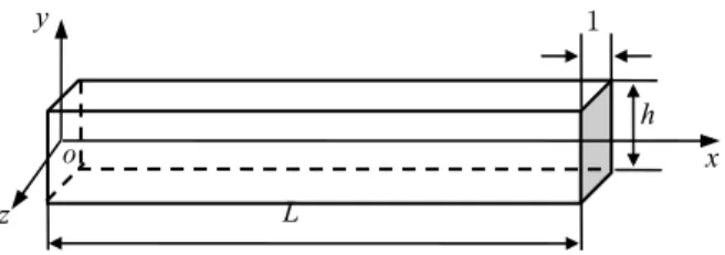
Figure 1: A straight beam of rectangular cross-section.
For a straight beam of rectangular cross-section, the coordinate system is shown in Figure 1. In the present work, according to the quantities in the plane elasticity theory, moment M, shear force Q, deflection w and rotation ϕ for a beam are respectively defined as
( )
( )
1
( )
1
( )=
x A
xy A
A
A
M x
y
dA
Q x
dA
w x
vdA
A
x
yudA
I
(1)
where x , y and xy are the stress components in the x-y plane. u(x, y) and v(x, y) are respectively
the axial and transverse displacements in this plane. A and I are respectively the area and the mo-ment of inertia of cross section. It is easily seen that definitions for M, Q and w are the same as often while the definition for rotation is somewhat different.
In this context, in parallel to Eqs. (1), the beam theory will be also established from the plane elasticity theory. Ignoring body forces, the governing equations in the plane elasticity theory are
x y
z
o
L
1
in the direction
in the direction
0
0
xy x
y yx
x
y
x
y
y
x
(2)
Taking the end of x=0 as an example, the corresponding boundary conditions are
in the direction in the direction
(0, ) given or
(0, ) given
(0, ) given or
(0, ) given
x
xy
x y
u
y
y
v
y
y
(3)In the x-direction, integration of the first of Eqs. (2) and (3) weighted by yover the cross sec-tion yields
0
xy x
A A
d
y
dA
y
dA
dx
y
(4)and
0
or
x 0A
yudA
Ayu dA
Ay
dA
Ay
dA
(5)In a similar manner, in the y-direction, integratingthe second of Eqs. (2) and (3) over the cross section, we have
+
y=0
yx
A A
d
dA
dA
dx
y
(6)and
0
or
xy 0A
vdA
Av dA
A
dA
A
dA
(7)Considering the first two of Eqs. (1), Eqs. (4) and (6) yield
0
+ ( )=0
M
Q
Q q x
(8)with
( )
yA
q x
dA
y
(9)
in the direction in the direction
0 given or
0 given
0 given or
0 given
x y
M
w
Q
(10)With Eqs. (10), all the practical boundary conditions in the x-direction and/or in the y-direction can be prescribed. For instance, we have
Free condition : and
Simply supported condition : and Fixed condition : and
0 given
0 given
0 given
0
0
0
0
0
0
M
Q
M
w
w
(11)
It should be noted that, due to the definitions in Eqs. (1), Eqs. (11) can also serve as the boundary conditions in the plane elasticity theory.
For a beam structure, the fundamental assumption is that y<< xy << x (e.g. see Ghugal and
Sharma, 2011), so, from the first of Eqs. (1), in terms of ϕ, the moment can be further expressed as
M
EI
(12)Together with Eqs. (8), the governing equations read
0
EI
q x
EI
Q
(13)3 THE KINEMATICS
3.1 The Unified Higher-Order Shear Deformation Model
In the second of Eqs. (13), Q must be expressed in terms of w(x) and/or ϕ(x). To this end, first, as often, the transverse displacement is assumed to be independent of the thickness coordinate y, and hence we have
,
( )
v x y
w x
(14)Next, the axial displacement is assumed to be expressed by
,
1( )
( )
R( )
u x y
y f x
g y
f
x
(15)where y and g(y) are respectively called the first-order term and the fundamental higher-order term with respect to y while f1(x) and fR(x) are the corresponding coefficient functions with respect to x.
It is worth noticing that g(y) is a pure higher-order term in this context. Substituting Eq. (15) into the fourth of Eqs. (1) yields
1 R
( )
x
f x
( )
f
( )
x
(16)
1
( )
A
I
yg y dA
(17)If we take fR(x)≡0, together with Eq. (16), Eq. (15) reduces to the first-order shear deformation
model as
,
( )
u x y
y
x
(18)For a higher-order model, upon eliminating fR(x) via Eq. (16), Eq. (15) becomes
1
( )
( )
1u
y f x
g y
x
f x
(19)Thus, considering Eq. (14), the shear strain over the cross section is
, , 1
( )
1xy
u
yv
xf
w
dg y dy
f
(20)For a beam of rectangular cross section, the shear stress free condition is often adopted on the top and bottom surfaces, which requires
,
2 0
xy
x
h
(21)So, from Eq. (20), we have
1
c
w
f
c
(22)where
y h2
y h2c
dg dy
dg dy
(23)Eventually, the axial displacement in Eq. (15) becomes
( )
c
w
g y
u
y
w
c
c
(24)Eq. (24) is termed as the unified HSD model for a beam corresponding to the fundamental higher-order term g(y).
Thus far, from Eqs. (23) and considering the higher-order property, g(y) has the following prop-erties
0 0
2 2
0
0
y
y
y h y h
g y
dg dy
dg dy
dg dy
(25)
( )
A xy PQ x
G
dA
K GA
w
(26)where KP, the shear correction factor originally defined by Timoshenko (1922,1921), takes the form
of
P
1
AK
c
dg dy dA
A c
(27)It can be seen from Eq. (27) that the shear correction factor will be certainly determined as long as g(y) is known, rather than other procedures (e.g. Cowper, 1966; Hutchinson, 2001).
If we assume
0
w
(28)Eq. (26) yields
( ) 0
Q x
(29)which implies that the shear effect cannot be not taken into account. Accordingly, Eq. (24) reduces to
,
( )
u x y
y w x
(30)which is the axial displacement assumption in the EBT (Dym and Shames,1973). Compared with the first-order shear deformation model in Eq. (18), the EBT in Eq. (30) is obtained under the ad-ditional assumption of Eq. (28), which is a more reasonable explanation than that of an infinite shear rigidity (e.g. Challamel, 2013).
3.2 Four Commonly Used HSD Models
One direct choice of the fundamental higher-order term is to take gA(y)=y 3. This model is just the commonly used third-order model and denoted as Model-A in this context. Eq. (27) yields
5 6
A P
K
(31)In this paper, other three commonly used HSD models are studied as well.
3.2.1 The Sine Model – Model-B
Inspired by Touratier (1991) and considering Eqs. (25), as the sine model, the fundamental higher-order term is taken to be
( )
sin
B
h
y
g
y
y
h
(32)3
24
1
1
c
(33)
So, the axial displacement in Eq. (24) yields
2
sin
24
B
h
y
u
yw
w
h
(34)Further, Eq. (27) yields
2
12
BP
K
(35)3.2.2 The Hyperbolic Sine Model – Model-C
Inspired by El Meiche et al. (2011) and Soldatos (1992) and considering Eq. (25), as the hyperbolic sine model, the fundamental higher-order term is taken to be
( )
sinh
C
y
g
y
y
h
h
(36)Accordingly, from Eqs. (17) and (23), we have
1 12 cosh(1 2) 2 sinh(1 2)
1 cosh(1 2)
c
(37)So, the axial displacement in Eq. (24) yields
cosh(1 2)
sinh(
)
24 sinh(1 2) 11 cosh(1 2)
C
y
h
y h
u
yw
w
(38)Further, Eq. (27) yields
cosh(1 2) 2sinh(1 2)
24sinh(1 2) 11cosh(1 2)
C P
K
(39)3.2.3 The Exponential Model– Model-D
Inspired by Karama et al. (2003) and considering Eq. (25), as the exponential model, the fundamen-tal higher-order term is taken to be
2( )
exp 2
D
g
y
y
y
y h
(40)1 3 exp( 1 2) (3 2 2)
( 2 2)
1
erf
c
(41)where the Gauss error function is defined as
2 0
2
( )
xexp(
)
erf x
s ds
(42)So, the axial displacement in Eq. (24) yields
2
exp 2 (
)
3exp( 1 2) (3 2 2)
( 2 2)
D
y
y h
w
u
yw
erf
(43)Further, Eq. (27) yields
exp( 1 2)
3exp( 1 2) (3 2 2)
( 2 2)
D P
K
erf
(44)3.3 Comparison of the Four HSD Models
3.3.1 The First-Order Term and the Third-Order Term Through Taylor’s Expansion
It is interesting to study the difference of the four HSD models by comparing the first two leading terms through Taylor’s expansion.
For the third-order model, the axial displacement is
,
1
235
4
3
A
y
u
x y
y
y
w
w
h
(45)Thus, if the axial displacement is expanded in form of power series
3
5 5
1 2 3
,
y
u x y
y
yc w
c w
O y
h
w
h
(46)from Taylor’s expansion, we have
1 3 3 5 1 3 1 3 1 3For Model - A For Model - B
For Model - C
Fo
1 4; 5 3
24 1; 144
cosh 1 2 1 24sinh 1 2 11cosh 1 2 1 1 6 24sinh 1 2 11cosh 1 2
1 3exp 1 2 3 2 2 2 2 1
2 3exp 1 2 3 2 2 2 2
A A B B C C D D c c c c c c c erf c erf
r Model - D
The coefficients are summarized in Table 1. It is seen that c3 increases with c1.
Model type c1 c3
Model-A 0.250 1.667
Model-B 0.292 2.125
Model-C 0.246 1.628
Model-D 0.338 2.676
Table 1: Comparison of the four HSD models in c1 and c3 3.3.2 Shear Correction Factors
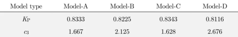
As already indicated in Section 3.1, given g(y), the shear correction factor can be evaluated for the beam of rectangular cross section. Values of the shear correction factor for the four HSD models in Section 3.2 are summarized in Table 2. It is seen that they vary a bit with different HSD models. In addition, KP becomes smaller if the HSD model (i.e. Model-D with the biggest c3) is farther
deviat-ed from the first-order shear deformation model.
Model type Model-A Model-B Model-C Model-D
KP 0.8333 0.8225 0.8343 0.8116
c3 1.667 2.125 1.628 2.676
Table 2: Comparison of the four HSD models in KP
From Eqs. (31) and (35), we can see that the commonly used shear correction factors can be reasonably explained by Eq. (27) in the manner of HSD models. For example, the TBT with KP
=5/6 (e.g. Kaneko, 1975; Timoshenko, 1922, 1921; Murthy, 1981; Reissner, 1975; Shi, 2007, 2011) is in essential equivalent to the third-order model (i.e. Model-A) because of Eq. (31) while the Mindlin plate theory (Mindlin, 1951) with KP =π2/12 is in essential equivalent to the sine model (i.e.
Model-B) because of Eq. (35).
4 THE UNIFIED SOLUTION
4.1 Derivation of the Unified Solution
In this section, the unified solution will be derived for the unified HSD model in Section 3. To this end, the governing equations are re-arranged as follows
0
P
EI
q x
EI
K GA
w
(48)
P
q x
EI
EI
w
K GA
(49)
From the first of Eqs. (49) - a third-order differential equation, the rotation ϕ can be first ob-tained, and then, from the second of Eqs. (49) – a first-order differential equation, the deflection w
can be further obtained.
In this context, a more general approach is used instead. To this end, Eqs. (48) are re-expressed as
(4)
( )
P
P P
q x
q x
w
EI
K GA
q x
EI
w
w
K GA
K GA
(50)
From the first of Eqs. (50), w is firstly obtained by solving a fourth-order differential equation, and ϕ is then directly obtained from the second of Eqs. (50). Eventually, we have
3 2
1 2 3 4
0 0 0 0 0 0
2 1
1 2 3
0 0 0
1
( )
1
( )
6
1
( )
3
2
x x x x x x
P
x x x
P
w
dx dx dx q x dx
dx q x dx a x
a x
a x a
EI
K GA
EIa
dx dx q x dx
a x
a x
a
EI
K GA
(51)
Figure 2: A cantilever beam under an arbitrarily distributed load
For the problem shown in Figure 2, the boundary conditions are
free condition at
0 :
(0) 0 ,
(0)
(0)
0
fixed condition at
:
( ) 0 , ( ) 0
P
x
EI
K GA
w
x
L
L
w L
(52)y
1
q(x)
x
So, the integration constants in Eqs. (51) are finally determined as
1
0 0
2
0 0 0
3
0 0 0 0 0 0
2
0 0 0 0
4
0 0 0 0
1 ( )
6
1 ( )
2
1 ( ) ( )
1
( ) ( )
2
1 ( )
x
x x x
x
x x x x x
x L x
x x
x x
x x x x
a q x dx
EI
a dx q x dx
EI
L
a dx dx q x dx dx q x dx
EI EI
L
q x dx q x dx
EI KGA
a dx dx dx q x dx EI
0 0 0
2 3
0 0 0 0 0
0 0 0 0
( )
( ) ( )
2 3
1 ( ) ( )
x x x
x L x L
x x x
x x
x x x
P x L P x
L
dx dx q x dx EI
L L
dx q x dx q x dx
EI EI
L
dx q x dx q x dx
K GA K GA
(53)Eqs. (51) and (53) are the unified solution for the beam problem shown in Figure 2.
The unified solution is also derived in Appendix A (see Eqs. (A.24) and (A.26)) by using the conventional beam theory. It is seen that Eqs. (A.24) will turn into Eqs. (51) if αT=1 (and hence
KT=KP from Eq. (A.13)). However, the fact is that αT is actually much less than unity for all the
HSD models (see Table A.1), leading to major difference between KT and KP. This may be the
reason why KT was not recognized as the shear correction factor in the previous HSD models (e.g.
Akgöz and Civalek, 2014a, 2014b; El Meiche et al., 2011; Huang et al., 2013; Levinson, 1987, 1981; Simsek, 2010; Touratier, 1991) despite of the definition already made as early as in 1920s (Timo-shenko, 1922,1921).
4.2 Comparison of the Results
With the unified solution, the results can be comparatively studied in detail. For this purpose, the special case of q=const is considered. From Eqs. (51) and (53), it is not difficult to obtain the uni-fied solution to this case as
4 3 4 2 2
3 3
4
3
24
2
6
Pq
q
w
x
L x
L
x
L
EI
K GA
q
x
L
EI
(54)
4 2
4 2 2
2 2
3
3 2
3 3 3 2
1 4 3 24 7 12 5 120
5 12 17 20
1 6 3 4 40 3 4 5 20
1 24 1 4 + 6
q Ref
q Ref
w vda qL x L x L EI qL h x L x L EI
A
qL x L x L GA
u y qL x L EI qLh x L EI qL x L GA
qLh x L EI qLh x L GA qxy EI qxy GAh
(55)
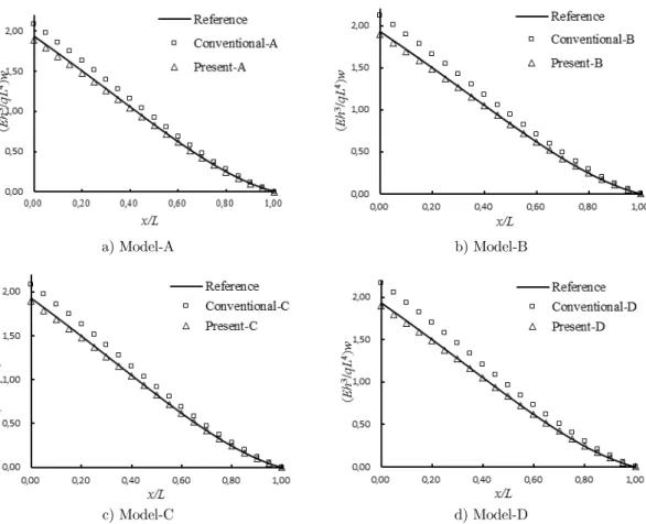
The deflections from different solutions are plotted in Figure 3 for the four HSD models in which “Reference”, “Conventional” and “Present” denote the solution from Eqs. (55), (A.27) and (54), respectively. It is seen that the current solution can always agree better with the reference for all the four HSD models than the conventional solution.
With Eqs. (51), the axial displacement (i.e. the warping of the cross section) can also be ob-tained through Eq. (24). The variation with y at x=L is plotted in Figure 4. It is seen that the warping from all the four HSD models are in considerably good agreement with the reference for the present solution. However, due to the apparent difference between KP and KT (see Table 2 and
Table A.1), the conventional solution greatly deviates.
a) Model-A b) Model-B
c) Model-C d) Model-D
a) Model-A b) Model-B
c) Model-C d) Model-D
Figure 4: Comparison of the warping of cross section from the four HSD models.
5 CONCLUSIONS AND FUTURE WORK
In this paper, with the definitions of average deflection and average rotation, the governing equa-tions and the boundary condiequa-tions were derived from the plane elasticity theory. Based on the kin-ematics in axial displacement, the unified HSD model was proposed by using the fundamental high-er-order term with some properties. The shear correction factor was then derived. The unified solu-tion was finally obtained for the unified HSD model subjected to an arbitrarily distributed load, and compared with the conventional one. From the current work, following conclusions can be made.
1)The definition of rotation plays an important role for the HSD models.
2)The kinematics of HSD models in axial displacement can be expressed by using the funda-mental higher-order term with some properties.
3)Given a loading, the unified solution can be derived for a beam with different fundamental higher-order terms in axial displacement.
The beam theory used in the current work is a lower-order (fourth-order) one in terms of deflec-tion w. Future work will focus on a variationally consistent higher-order (sixth-order) beam theory and the shear correction factor of arbitrary cross section. Application to small scale problems and extension to a plate problem are also prospective.
Acknowledgements
This work was supported by the National Natural Science Foundations of China (Grant Nos. 11272245, 11321062)
References
Akavci, S.S., Tanrikulu, A.H., (2008). Buckling and free vibration analyses of laminated composite plates by using two new hyperbolic shear-deformation theories. Mechanics of Composite Materials 44: 145-54.
Akgöz, B., Civalek, O., (2014a). Shear deformation beam models for functionally graded microbeams with new shear correction factors. Composite Structures 112: 214-25.
Akgöz, B., Civalek, O., (2014b). A new trigonometric beam model for buckling of strain gradient micro beams. In-ternational Journal of Mechanical and Sciences 81: 88-94.
Akgöz, B., Civalek, O., (2015). A novel microstructure-dependent shear deformable beam models. International Journal of Mechanical and Sciences 99: 10-20.
Aydogdu, M., (2009). A new shear deformation theory for laminated composite plates. Composite Structures 89: 94– 101.
Bickford, W.B., (1982). A consistent higher order beam theory. In: Developments in Theoretical and Applied Me-chanics. vol. XI. University of Alabama, Alabama.
Challamel N., (2011). Higher-order shear beam theories and enriched continuum. Mechanics Research Communica-tions 38(5): 388-92.
Challamel N., (2013). Variational formulation of gradient or/and nonlocal higher-order shear elasticity beams. Com-posite Structures 105: 351–68.
Cowper, G.R., (1966). The shear coefficient in Timoshenko’s beam theory. Journal of Applied Mechanics-Transactions of the ASME 33: 335-40.
Dong, S.B., Alpdogan, C., Taciroglu, E., (2010). Much ado about shear correction factors in Timoshenko beam theo-ry. International Journal of Solids and Structures 47: 1651-65.
Dong, S.B., Çarbaş, S., Taciroglu, E., (2013). On principal shear axes for correction factors in Timoshenko beam theory. International Journal of Solids and Structures 50: 1681-8.
Dym, C.L., Shames, I.H., (1973). Solid Mechanics: A Variational Approach. McGraw-Hill (New York).
El Meiche, N., Tounsi, A., Ziane, N., Mechab, I., Bedia, EA., (2011). A new hyperbolic shear deformation theory for buckling and vibration of functionally graded sandwich plate. International Journal of Mechanical and Sciences 53: 237-47.
Ghugal, Y.M., Sharma, R., (2011). A refined shear deformation theory for flexure of thick beams. Latin American Journal of Solids and Structures 8: 183-95.
Guttmann, F., Sauer, R., Wagner, W., (1999). Shear stresses in prismatic beams with arbitrary cross section. Inter-national Journal for Numerical Methods in Engineering 45: 865-89.
Guttmann, F., Wagner, W., (2001). Shear correction factors in Timoshenko's beam theory for arbitrary shaped cross-section. Computational Mechanics 27: 199-207.
Hutchinson, J.R., (2001). Shear Coefficients for Timoshenko Beam Theory. Journal of Applied Mechanics-Transactions of the ASME 68: 87-92.
Jensen, J.J., (1983). On shear coefficient in Timoshenko's beam theory. Journal of Sound and Vibration 87: 621-35. Kaneko, T., (1975). Timoshenko’s correction for shear in vibrating beams. Journal of Physics D-Applied Physics 8, 1927-36.
Karama, M., Abou Harb, B., Mistou, S., Caperaa, S., (1998). Bending, buckling and free vibration of laminated composite with a transverse shear stress continuity model. Composites Part B: Engineering 29B, 223-34.
Karama, M., Afaq, K.S., Mistou, S., (2003). Mechanical behavior of laminated composite beam by the new multi-layered laminated composite structures model with transverse shear stress continuity. International Journal of Solids and Structures 40: 1525-46.
Levinson, M., (1981). A new rectangular beam theory. Journal of Sound and Vibration 74: 81-7.
Levinson, M., (1987). On higher order beam and plate theories. Mechanics Research Communications 14, 421-24. Mantari, J.L., Oktem, A.S., Guedes Soares, C., (2012). A new trigonometric shear deformation theory for isotropic, laminated composite and sandwich plates. International Journal of Solids and Structures 49: 43-53.
Mindlin, R.D., (1951). Thickness-shear and flexural vibrations of crystal plates. Journal of Applied Physics 22: 316-23.
Murthy, M.V.V., (1981). An Improved Transverse Shear Deformation Theory for Laminate Anisotropic Plates. NA-SA Technical Paper No. 1903.
Pai, P.F., Schulz, M.J., (1999). Shear correction factors and an energy-consistent beam theory. International Journal of Solids and Structures 36: 1523-40.
Reddy, J.N., (1984a). A refined nonlinear theory of plates with transverse shear deformation. International Journal of Solids and Structures 20: 881-96.
Reddy, J.N., (1984b). A simple higher-order theory for laminated composite plates. Journal of Applied Mechanics-Transactions of the ASME 51: 745-52.
Reissner, E., (1975). On transverse bending of plates, including the effect of transverse shear deformation. Interna-tional Journal of Solids and Structures 11: 569-73.
Rohwer, K., (1992). Application of higher order theories to the bending analysis of layered composite plates. Interna-tional Journal of Solids and Structures 29: 105–19.
Shi, G.Y., (2007). A new simple third-order shear deformation theory of plates. International Journal of Solids and Structures 44: 4399-417.
Shi, G.Y., (2011). A Sixth-Order Theory of Shear Deformable Beams With Variational Consistent Boundary Condi-tions. Journal of Applied Mechanics-Transactions of the ASME 78(021019): 1-11.
Simsek, M., (2010). Fundamental frequency analysis of functionally graded beams by using different higher-order beam theories. Nuclear Engineering and Design 240: 697-05.
Soldatos, K.P., (1992). A transverse shear deformation theory for homogeneous monoclinic plates. Acta Mechanica 94: 195-220.
Timoshenko, S.P., (1921). On the correction for shear of the differential equation for transverse vibration of pris-matic bars. Philosophical Magazine 41, 744-46.
Timoshenko, S.P., (1922). On the transverse vibrations of bars of uniform cross-section. Philosophical Magazine 43: 125-31.
Timoshenko, S.P., Goodier J.N., (2004). Theory of Elasticity, Tsinghua University Press. Beijing, China.
Wang B.L., Liu M.C., Zhao J.F., Zhou S.J., (2014). A size-dependent Reddy-Levinson beam model based on a strain gradient elasticity theory. Meccanica 49(6): 1427-41.
Wang C.M., Kitipornchai S., Lim C.W., Eisenberger M., (2008). Beam bending solutions based on nonlocal Timo-shenko beam theory. Journal of Engineering Mechanics-Transactions of the ASCE 134(6): 475-81.
APPENDIX A: THE CONVENTIONAL BEAM THEORY WITH THE UNIFIED HSD MODEL AND THE UNIFIED SOLUTION
A.1 Governing Equations and Boundary Conditions
In the conventional beam theory, deflection
w x
( )
and rotation ψ(x) are defined as (e.g. Timoshen-ko and Goodier, 2004)
0( )
,0
( )=
y
w x
v x
x
u y
(A.1)
With the assumption of Eq. (15),
w x
( )
is identical to w(x).Together with the properties in the first two of Eqs. (25) for g(y), Eq. (15) is still mathematical-ly valid. Thus, the shear strain is
1( )
( )
R( )
xy
u
v
f x
w x
dg dy
f
x
y
x
(A.2)Considering the shear stress free condition on the top and bottom surfaces
1
R( ,
2)
( )
( )
( ) 0
xy
x
h
f x
w x
c f
x
(A.3)we have
R
( )
1
1( )
( )
f
x
f x
w x
c
(A.4)where c is as defined in Eq. (23) and hence the property in the third of Eqs. (25) stand also for g(y). From the definition in the second of Eqs. (A.1) and considering the third of Eqs. (25), we have
1
( )
x
f x
( )
(A.5)
( , )
u x y
y
g y
c
w
y w
y
g y
c
w
(A.6)As often, Eq. (A.6) can also be re-expressed as
( , )
u x y
y w
S y
w
(A.7)with
S y
y
g y
c
(A.8)Based on Eqs. (25), S(y) has following properties
0 0
2
0
1
0
y
y
h y
S y
dS dy
dS dy
(A.9)
From Eq. (A.7), we further obtain
(
)
T
Q
K GA
w
(A.10)with
1
( )
T
K
dS y dy dA
A
(A.11)In addition, in terms of
w x
( )
and ψ(x) (Aydogdu , 2009; Akavci and Tanrikulu, 2008; El Meiche et al., 2011; Karama et al., 1998, 2003; Levinson, 1981; Mantari et al., 2012; Soldatos, 1992; Touratier, 1991), moment M can be expressed in a unified form as
T
M
EIw
EI
w
(A.12)with
1
( )
T
I
y S y dA
Interestingly, we can obtain the following relationship
T T P
K
K
(A.14)From Eqs. (A.10) and (A.12), in terms of
w x
( )
and ψ(x), the governing equations are
0
T
T T
K AG
w
q x
EIw
EI
w
K AG
w
(A.15)with the boundary conditions as [e.g. Levinson, 1981]
0 0
0 0
0 0
Free condition :
and
Simply supported condition :
and
0
Fixed condition :
0 and
0
M
M
Q
Q
M
M
w
w
w
w
(A.16)
A.2 The Four Commonly Used HSD Models
(1) The third-order model – Model-A (Levinson, 1981)
In the third order shear deformation model, we take gA(y)=y3, and hence c=3h2/4 from Eq. (23). Then, Eq. (A.8) yields
2 2
4
( )
1
3
A
y
S
y
y
h
(A.17)(2) The sine model – Model-B (Touratier, 1991)
In this HSD model, gB(y) takes the form of Eq. (32), and hence c=1 from Eq. (23). Then, Eq. (A.8) yields
( )
sin
B
h
y
S
y
h
(A.18)(3) The hyperbolic sine model – Model-C (Soldatos, 1992)
In this HSD model, gC(y) takes the form of Eq. (36), and hence c=1-cosh(1/2) from Eq. (23). Then, Eq. (A.8) yields
cosh 1 2
sinh
( )
cosh 1 2 1
C
y
h
y h
S
y
(A.19)It should be noted that Eq. (A.19) firstly derived according to Eqs. (A.8) corrects the original form in Soldatos (1992).
(4) The exponential model – Model-D (Karama et al., 2003)
2 2
( )
exp 2 /
D
S
y
y
y
h
(A.20)A.3 Shear Correction Factors
From Eq. (A.11), for the four HSD models, it is immediate to obtain
2 3
2
cosh(1 2) 2sinh(1 2)
cosh 1 2 1
exp 1 2
T
T
T
T A
B
C
D
K
K
K
K
(A.21)
In addition, from Eq. (A.13), we have
3
4 5
24
24sinh(1 2) 11cosh(1 2)
cosh 1 2 1
3exp( 1 2) 3 2 2
2 2
A T
B T
C T
D
T
erf
(A.22)
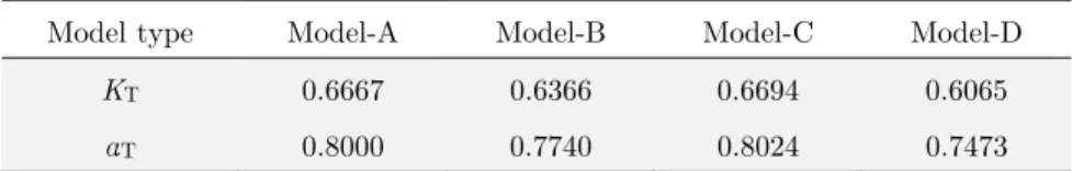
The values for KT and αT are summarized in Table A.1. Compared with KP in Table 2, Eq.
(A.14) can also be validated by the four HSD models.
Model type Model-A Model-B Model-C Model-D
KT 0.6667 0.6366 0.6694 0.6065
αT 0.8000 0.7740 0.8024 0.7473
Table A.1: Comparison of the four HSD models in KT and αT. A.4 The Unified Solution
For sake of the unified solution, Eqs. (A. 15) are further re-expressed as
(4) T
T
T
T T
q
x
q x
w
K AG
EI
q x
EI
w
w
K AG
K AG
(A.23)
3 2
1 2 3 4
0 0 0 0 0 0
2
1 2 1 3
0 0 0 0
1
( )
( )
1
1
( )
( )
3
2
6
x x x x x x
T
T
x x x x
T
T T
w
dx dx dx q x dx
dx q x dx b x
b x
b x b
EI
K AG
EI
dx dx q x dx
q x dx
b x
b x
b
b
EI
K AG
K AG
(A.24)For the problem shown in Figure 2, from Eqs. (A.16), the corresponding boundary conditions for the conventional beam theory are
Free condition at
0 :
(0)
(0)
(0)
0
(0)
(0)
0
Fixed condition at
:
( ) 0 , ( ) 0
T
T
x
EIw
EI
w
K GA
w
x
L
L
w L
(A.25)Thus, the integration constants in Eqs. (A.24) are determined as
1
0 0
2
0 0 0
2 3
0 0 0 0 0 0 0 0
0 0 0
4
1
( )
6
1
( )
2
1
( )
( )
( )
2
1
( )
1
( )
1
x
x
x x
x
x x x x x x
x L x x
x x
T
T x L T x
b
q x dx
EI
b
dx q x dx
EI
L
L
b
dx dx q x dx
dx q x dx
q x dx
EI
EI
EI
q x dx
q x dx
K AG
K AG
b
E
0 0 0 0 0 0 0
2 3
0 0 0 0 0
0 0 0 0
( )
( )
( )
( )
2
3
1
( )
( )
( )
x x x x x x x
x L x L
x x x
x x
x x x x
T T
T x L T T x
x L
L
dx dx dx q x dx
dx dx q x dx
I
EI
L
L
dx q x dx
q x dx
EI
EI
L
dx q x dx
L
q x dx
q x dx
K AG
K AG
K AG
0
(A.26)
4 3 4 2 2
3 3
1
4
3
24
2
1
6
T T
T
T T
T
T
qL
q
q
w
x
L x
L
x
L
x
L
EI
K AG
K AG
q
q
x
L
x
L
EI
K AG
(A.27)