Lat. Am. j. solids struct. vol.14 número11

Abstract

It is necessary to detect danger as soon as possible to avoid rollover of a vehicle in sudden events. Using rollover index in real time can be used for this purpose. The traditional rollover indices currently applying in the vehicles can only detect the untripped rollover due to severe lateral acceleration in vehicles. These indices cannot de-tect the tripped rollover resulted from vertical external forces in a long direction. There are recently many quantitative studies about the tripped rollover and an index was also introduced to this kind of rollover. In this research, we examined the dynamics of a SUV to improve this index and also presented a new index to detect the both types of rollovers. The precision and accuracy of the new index was evaluated by simulation in industrial software of Carsim. The numerical results of the new developed model were compared with the test results of an automobile at one-eighth scale in equal conditions and inputs. The results are indicative of the better per-formance of the new model presented in this research.

Keywords

Vehicle dynamics, Tripped rollover, Untripped rollover, Rollover index, Suspension system

Rollover Index for the Diagnosis of Tripped and Untripped Rollovers

1 INTRODUCTION

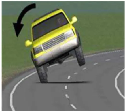
As the dimensions of vehicles increase, they are more possible to have rollover in different road con-ditions. The rollover may occur in one of two ways: tripped or untripped. Untripped rollover results from the high lateral acceleration in sharp turnings of road. On the other hand, tripped rollover may occur as a result of external vertical forces applied to the automobile

Amir Hossein Kazemian a,*

Majid Fooladi b

Hossein Darijani c

a _{Mechanical Engineering Department,}

University of Sistan and Baluchestan, Zahedan, Iran. kazemian@eng.usb.ac.ir

b _{Mechanical Engineering Department,}

Shahid Bahonar University of Kerman, Kerman, Iran. fooladi@uk.ac.ir

c _{Mechanical Engineering Department,}

Shahid Bahonar University of Kerman, Kerman, Iran. darijani@uk.ac.ir

* Corresponding Author

http://dx.doi.org/10.1590/1679-78253576

a) Tripped Rollover b) Untripped Rollover

Figure 1: Types of rollover.

Automobile rollovers considerably contribute to deathful driving accidents. In about 11 million accidents in passenger car, SUV, pickup and vans in 2010, only 3 percent of the accidents were re-lated to the rollover. However, close to 33 percent of all the mortality caused by accidents is result-ed from rollover(National Highway Traffic and Safety Board, 2011). Basresult-ed on information pub-lished by NHTSA in 2006, the accidents caused by rolling were observed in 70% of light vehicle accidents. Thus, in recent years, rollover is considered as an important safety issue for vehicles.

Figure 2: Statistical results of NHTSA (Phanomchoeng & Rajamani, 2012).

(SSF)(Dilich & John, 1997). It can also be used in roll angle as an index to detect the rollover, but it is not used as an independent index and usually applied as a supplementary factor (Hsu & Chen, 2012). Another important and useful criterion is automobile energy index. In this index, the kinetic energy of the vehicle is compared with the maximum amount of potential energy and its dynamics is controlled before it reaches this threshold (Johansson & Gafvert, 2004). Another index that is defined on the basis of forces between the tire and road is the index lateral load transfer. To deter-mine the index, the vertical force of left and right tires is calculated and if their difference passes the threshold, the controller is activated(R Rajamani, Piyabongkarn, Tsourapas, & Lew, 2009). Based on the angle between the tire contact force and road surface, rollover index is defined as a measure force-angle. Based on the mentioned criteria, various new indices can be created. For ex-ample, the criterion Time to Rollover (TTR) is defined based on roll angle and lateral pressure(Chen & Peng, 1999; Yoon, Kim, & Yi, 2007).

Selecting one of the rollover indices, vehicle dynamic stability can be obtained through the use of different control methods. Many researches presented a variety of mechanisms including different suspension systems (Cech, 2000), differential braking system, and steering control mechanism acti-vated by using different control methods in order to control vehicle rollover. Solmaz et al.(Solmaz, Corless, & Shorten, 2007) presented a method based on discrete-time systems in active steering control to analyze rolling dynamics of vehicles. Tavan et al. (2015) proposed an optimal controller for integrated longitudinal and lateral closed loop vehicle dynamics to follow desired path in various

driving maneuvers(Tavan, Tavan, & Hosseini, 2015). The design of a suspension system

emphasiz-es weight reduction (Kong, Abdullah, Omar, & Haris, 2016) Active and semi-active suspension sys-tems are kinds of automotive suspension mechanisms that control cyclic vertical movement of the car in a broad frequency range and energy waste through real-time feedback. Every moment the tires go up and down separately depending on the conditions of the road until the car's occupants will have the maximum comfort(Solmaz, Shorten, Wulff, & Cairbre, 2008).Pagnacco et al. designed an active suspension device to satisfy certain limitations in a given frequency(Pagnacco, Zidani, Sampaio, de Cursi, & Ellaia, 2016; Pan, He, Xiao, & Liu, 2016).

2 VEHICLE ROLLOVER INDEX

Vehicle rollover index is a real-time variable that can be used for wheel lift-off conditions. The basic definition of rollover R is described as:

zr zl zr zl F - F

R = -1 1

F + F R  (1)

Where Fzrand Fzlare the vertical force of right and left tires. When the vehicle is in a rollover

threshold, the index value is greater than 1 or less than 1. It is noteworthy that when the

automo-bile is moving in a straight road, both the Fzrand Fzlare equal and the rollover value is zero. As

zl

F 0, then R=1, and the vehicle just will be on the right tire on the surface. The relation 1 cannot

be implemented because the forces are not measureable. Many attempts have been conducted by researchers to obtain the indices. Many of the attempts resulted in the index based on lateral

accel-eration and untripped rollover. An applied formula of R rollover index can be based on anda_y .

1

2 s y R 2 s R tan( )

w w

m a h m h

R

m gL m L



  ₍₂₎

Wherem ms mu, hR is the height of center gravitymu is the unsprung mass, msis the sprung

mass, a_y is the lateral acceleration, and  is the rotation angle.This rollover index can just be

ap-plied to detect untripped rollover. Some studies defined the rollover index just based on lateral ac-celeration because it is difficult to find roll angle (Odenthal, Bunte, & Ackermann, 1999; Solmaz, Corless, & Shorten, 2006). The stability control with this index may reduce the ability of lateral movement of the vehicle and is not also able to detect the rollover resulted by vertical forces and road inputs.

2

2 s y R w

m a h R

m gL

 ₍₃₎

In commercial form of index, the acceleration of sprung mass is also considered separately (Rajesh Rajamani & Phanomchoeng, 2013).





3

2 s y R 2 s R tan( ) u ur ul

w w

m a h m h m z z

R

m gL m L m g

 

     ₍₄₎

Where



z

 

ur



z

ul



is the difference between the acceleration of unsprung masses.

Figure 3: tripped and untripped rollover model in 4 degrees of freedom suspension systems (Phanomchoeng & Rajamani, 2013).

























2 2

4

2 2 _{cos( ) sin( )}

2 u ur ul x x s R zl zr s R y

s s

u ur ul s s s u

m z z I m h a a m h a g

l l

R

m z z m z m m g

 

     



   

 

   (5)

Where



a

zl



a

zr



is the difference between acceleration of sprung mass and Ixxis the roll moment of

inertia around longitudinal axes.

According to the national highway safety administration (NHTSA), 95% of rollovers in single-seat vehicles are related to tripped rollover. Thus, development and improvement of these indicators have significant potential impact on technology.

Where



a

zl



a

zr



is the difference between acceleration of sprung mass and

I

xx is the roll

mo-ment of inertia around longitudinal axes.

According to the national highway safety administration (NHTSA), 95% of rollovers in single-seat vehicles are related to tripped rollover. Thus, development and improvement of these indicators have significant potential impact on technology.

3 IMPROVED ROLLOVER INDEX FOR TRIPPED AND UNTRIPPED ROLLOVERS

3.1 Rollover Index for 6 Degrees of Freedom Suspension Systems

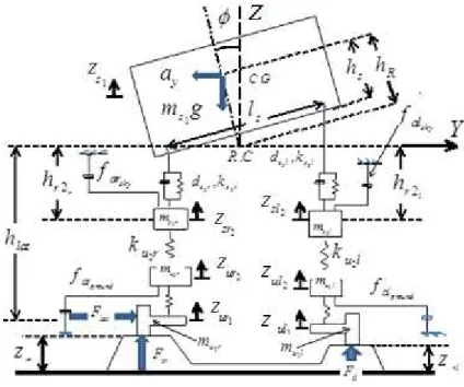
hybrid semi-active suspension system of 6 degrees of freedom using a magneto-rheological damper (Ahmadian, 2014) (Figure 4).

It should be noted that adding degrees of freedom is a way to assess its impacts on stability and

well controllability of the system. As represented in Figure 4, the

m

_u2represents the masses added

to the unsprung part of the automobile.

The 6 degrees of freedom suspension system in a vehicle is vertical movement of the sprung

mass in

z

s, rotation angle and vertical movements of right and left unsprung masses,



zu r1 ,zu l1 ,zu r2 ,zu l2



. Variables of zrrand zrl are road profiles that motivate the system and enter a

lateral force input Flat in a certain height hlatfrom the center of rotation. The external outputs of

rr

z , z_rl and F_latcannot be measured and thus, are unknown. However, these outputs depending on

these inputs can be measured. For example, lateral and vertical accelerations can be measured by different accelerometers. These lateral and vertical accelerations can be related to unknown inputs

or algebraic equations. Figure 4 represents these forces (



F F

zr

,

zl



).

Figure 4: A semi-active hybrid 6 degrees of freedom suspension system.

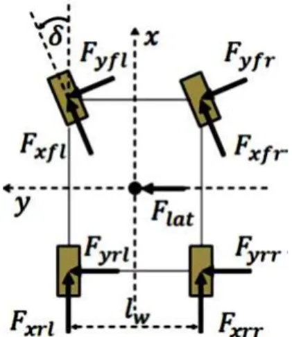
Figure 5: Lateral forces in schematic view.

 

 



yf cos x f sin yr lat



y

F F F F

a

m

    

 (6)

In this figure, the value

a

y is including of lateral tire forces and the unknown force of Flat

where, 2 2

1 i 1 j s u r u l

i j

m m m m

 

 







and F_xf is the longitudinal force in right and left fore-wheels,

F

yr

and

F

yf are the lateral forces of back and fore tires s in right and left, and



is the steering angle.

As the effects of road inputs are considered, the suspension forces on chassis are as follow:

1 total sky

sr sr ar

F



F



F

₍₇₎

1 total sky

sl sl al

F



F



F

₍₈₎

Where

F

sr₁and

F

sl1are passive suspension system forces and

F

arsky and

F

alsky are semi active damper

forces of a vehicle.

 

1 2 sin 2

s

sr sr s u r

l

F  k _z   z _

  (9)

 

1 2 sin 2

s

sl sl s u l

l

F  k _z   z _

  (10)

This is noteworthy that magneto-rheological (MR) has been used and the direct impacts of this

damper have been considered in a new index. Thus, the impacts of

F

ar_sky and

F

al_skyfrom the forces of

sr

F and F_slare also considered separately.

Applying the second principle of Newton law for the sprung mass leads to:

1 1 s k y s k y

s s s r s l a r a l s

Dynamic modeling of moving unsprung mass is carried out in two steps. First, the basic

dynam-ic equations are added to the two objects of

m

u r₂

,

m

u l₂ , and then, it is added to unsprung mass of

tires that are in direct contact with the ground.

Applying Newton's second law for the unsprung masses leads to:

2 2 1 1 2 arg r o u n d

u r ur s r ur u r

m z  F  F  m g  F ₍₁₂₎

As a result,

1 2 2 1 2 a rg r o u n d

u r u r ur s r u r

F  m z  F  m g  F ₍₁₃₎

Likewise, for the unsprung mass in left tire we have:

2 2 1 1 2 g r o u n d

ul u l s l ul u l a l

m z  F  F  m g  F ₍₁₄₎

Where,

1 2 2 1 2 g r o u n d

u l ul ul s l u l a l

F  m z  F  m g  F ₍₁₅₎

Thus, the dynamic equations of movement for the unsprung masses of tires are: In the right tire:

1 1 1 1

u r u r u r tr u r

m z





F

 

F

m g

₍₁₆₎

In the left tire:

1 1 1 1

u l u l u l tl u l

m z



 

F

 

F

m g

₍₁₇₎

By replacing the equations 13 and 14 in the equations 16 and 17, the result is:

1

1 2 2 1 2 1

`

ground

u r

u r ur ur sr u r tr u r ar

m z





m z





F



m g F

 

m g F



(18)

1

1 2 2 1 2 1

`

ul _ground

u l ul ul sl ul tl ul al

m z





m z





F



m g

 

F

m g



F

(19)

Therefore, for the new model in this study, the vertical forces can be calculated as:

1

1 2 2 1 2 1

`

ground

r r

u r

tr u r u u sr u r u r ar

F



m z





m z





F



m g



m g F



(20)

1

1 2 2 1 2 1

`

ground

l l

u l

tl u l u u sl u l u l al

F



m z





m z





F



m g



m g



F

(21)

























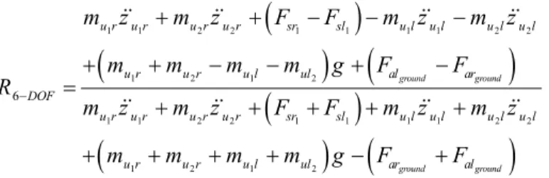
1 1 2 2 1 1 1 1 2 2

1 2 1 2

1 1 2 2 1 1 1 1 2 2

1 2 1 2

6

ground ground

ground ground

u r u r u r u r sr sl u l u l u l u l

u r u r u l ul

DOF

u r u r u r u r sr sl u l u l u l u l

u r u r u l ul

al ar

ar al

m z m z F F m z m z

m m m m g

R

m z m z F F m z

F F

F

m z

m m m m g F



    

    



    

   



 

   

    (22)

Where

F F

sr₁

,

sl₁ are replaced with Equations (9) and (10). Given that the parameters of the

forc-es are unknown and not easily measurable; this needs to remove the unknown parameters.

Calculat-ing the suspension system

F F

sr₁

,

sl₁by Equation (11) resulted in:



Fsr1 Fsl1



m zss m gs 



Farsk y Falsk y



(23)

The equation of rotation movement around the roll center (RC) leads to:







1 1







2 _{cos sin}

2 2 sky sky

s s

xx s R sl sr al ar s y R s R

l l

I m h  F F  F F m a h m gh  ₍₂₄₎

As a result,



1 1







 

 





2

2 _{sin cos}

2 sky sky s

sl sr xx s R s R s y R al ar

s

l

F F I m h m gh m a h F F

l   

 

  _      _

   (25)

The Zs parameter can be measured by an accelerometer. Theangle can be calculated by a tilt

angle sensor. One example of a tilt meter is the Crossbow CXTD02. This is consisted of two axis in-built accelerometers and a signal processing algorithm to calculate the angles of tilting. For exam-ple, one of the algorithms for this purpose is mentioned in (Rajesh Rajamani, 2011) . To calculate

the, two extra accelerometers are required to be placed at the right and left ends on an

automo-bile sprung mass.

The value of the right accelerometeraz ris obtained as:

 



  

 

cos sin cos

2

zr s x

ls

a z    yv   g  ₍₂₆₎

The left accelerometer is also obtained as:

 



  

 

cos sin cos

2

zl s x

ls

a z    yv   g  ₍₂₇₎

Where the component



y v





x







is the effect of the unknown forceFlat .

Figure 7: Schematic of lateral dynamics of a vehicle (Rajesh Rajamani, 2011).

By subtracting the equation 26 from the equation 27, we would reach:







z l z r



z l z r s

s

a a

a a l

l

  

    ₍₂₈₎

By replacing Equations 23, 25, and 28 with Equation 22, the left and right masses are assumed to be equal, and the rollover index of the vehicle with 6 degree of freedom suspension system leads to:





_

_









 

 









1 1 1 2 2 2

1 1 1 2 2 2

2 1 2 2 6 2 ( ) ( ) ( ) ( ) 2( ) 2

2 _{cos sin}

sky sky

ground ground

sky sky gro

xx s R

u u r u l u u r u l zl zr

s DOF

u u r u l u u r u l s s ar al

s

u u al ar

s R y ar al al

s

I m h

m z z m z z a a

l R

m z z m z z m z F F

m

m m g F F

m h a g F F F

l  

                                













1 1 1 2 2 2

2 1 ( ) ( ) 2( ) 2 und ground sky sky ground ground ar

u u r u l u u r u l s s ar al

s

u u al ar

F

m z z m z z m z F F

m

m m g F F



     

    

    

3.2 Rollover Index for Automobile Suspension System with 8 Degrees of Freedom

To improve the stability and controllability of a suspension system with increasing degree of free-dom, a new hybrid semi active suspension system with 8 degrees of freedom has been designed in combination with a semi-active hybrid suspension system with 6 degrees of freedom and a passive suspension system with 4 degrees of freedom. To do so, we added two symmetrical equal masses to the sprung part and also used MR damper of the hybrid suspension system with 8 degrees of

free-dom. As can be observed in Figure 8,

m

s₂ represents the added masses to the sprung part.

Figure 8: A hybrid semi-active 8 degrees of freedom suspension system.

According to the previous arguments and based on Equation 6, the value of lateral acceleration

including the effects of lateral forces and the force of Flat can be seen as:

 

 



yf cos x f sin yr lat



y

F F F F

a

m

    

 (30)

Where

m





m

_s





m

_u

The suspension forces exerted on the chassis include

total sky

sr sr ar

F



F



F

₍₃₁₎

total sky

sl sl al

F



F



F

₍₃₂₎

 

 

1 2 sin 2 1 2 cos 2

s s

sr sr s s r sr s s r

l l

F  k _z   z _d _z    z _

      (33)

 

 

1 2sin 2 1 2 cos 2

s s

sl sl s s l sl s s l

l l

F  k _z   z _d _z    z _

       (34)

By assuming that the suspension forces always act vertically, the sprung mass 1 roll motion is given by:



1 1











1

 

1

 

2

1 1

g sin cos

2 2 sky sky

s s

xx s R sl sr al ar s R s y R

l l

I m h  F F  F F m h  m a h  ₍₃₅₎

By applying Newton's second law to the chassis:

1 1 1

s s sr s l arsky alsky s

m z





F



F



F



F



m g

₍₃₆₎

Similarly, for the added sprung masses:

2 2 sky 2 2

(

2 2

)

s r s r sr ar s r u r s r u r

m z



  

F

F



m g



k

z



z

₍₃₇₎

2 2 sky 2 2

(

2 2

)

s l s l sl al s l u l s l u l

m z



 

F



F



m g



k

z



z

₍₃₈₎

Dynamic modeling of the unsprung mass movement is conducted in two stages. In the first

stage; basic dynamic equations for the added unsprung masses

m

u r₂

,

m

u l₂ , and in the second stage,

the dynamic equations are considered for the unsprung masses of tires

m

u r₁

,

m

u l₁ in contact with the

ground surface.

It must be kept in mind that the terms of

k

u r₂

(

z

s r₂



z

u r₂

)

and

k

u l2

(

z

s l2



z

u l2

)

are appropriate

to exchanged forces to the sprung part and those added to the unsprung part. The two terms are called

F

(r s)rand

F

(r s)l, respectively.

With the second law of Newton for the added unsprung masses, we have:

2r 2r (r ) 1 2 arground

u u sr u r ur

m z



 

F

_



F



m g



F

₍₃₉₎

2l 2l (r )l 1 2 ground

u u s u l ul al

m z



 

F





F



m g



F

(40)

As a result:

1 2r 2r (r s) 2 arground

u r u u r ur

F



m z





F

_



m g



F

₍₄₁₎

1 2l 2l (r s)l 2 ground

u l u u u l al

F



m z





F





m g



F

(42)

1 1 1 1

u r u r u r tr u r

m z  F  F m g ₍₄₃₎

Left tire:

1 1 1 1

u l u l u l tl u l

m z  F F m g ₍₄₄₎

By replacing the equations 41 and 42 in the equations 43 and 44, the result is:

1

1 2 2 2 1

`

( )

u r _ground

u r ur u r r s r u r ar tr u r

m z  m z  F _ m g F  F m g (45)

1 1 2 2 2 1

`

( ) l

ul grou dn

u l u l ul r s ul al tl ul

m z  m z  F  m g F F m g (46)

Now, for the new model presented in this research, the vertical forces of the tires can be calcu-lated as:

1

1 2 2 2 1

`

( )

u r _ground

tr u r u r ur r s r u r u r ar

F  m z m z F _ m gm gF (47)

1

1 2 2 2 1

`

( ) l

u l _ground

tl u l ul ul r s u l u l al

F m z m z  F _ m gm gF (48)

It is noteworthy that in this stage, a relationship in the forcesF(rs r) _, F(rs) l_, Fsr1, Fsl1 should be

chosen to be exerted in the rollover index with the 8 degrees of freedom suspension system. So from the equations 37 and 38, we have:

2 2 2

(r s r) sr arsky s r s r s r

F





F



F



m g



m z



(49)

2 2 2

(r s)l sl alsky s l s l s l

F

_



F



F



m g



m z



₍₅₀₎

By substituting the equations 49 and 50 in the equations 47 and 48, the result is:

1

1 2 2 2 2 2 2 1

`

u r

grou

ky d

s n

tr u r u r u r Fsr Far msrg msrzs r u r u r ar

F  m z  m z       m g m g F (51)

1

1 2 2 2 2 2 2 1

`

s

u l _{ky ground}

tl u l ul u l Fsl Fal ms lg s l s l u l u l al

F m z m z    m z m gm g F (52)

Since the vertical forces of Ftr,Ftlare equal to those ofFz r,Fz l, the rollover index, by assuming

equality in the mass of the left and right suspension system is:















 



















1

1 1 2 2 2

1 1

2 2 2

2 2 2

2 2 2

1 ` ` ` ` u l u r ground ground u l u r gr sky sk ou y

sky sky nd

r l s s r s l

sr sl ar al

r l s s r s l sr sl

ar al

u u u u

al ar

u u u u

ar al

m z z m z z

F F

m z z

F F F F

R

m

m z z m z z

F

z z F

F F F

F    _{ }                     _{  }                     



ground



2



ms2 mu2 mu1



g

The unknown forces of Fsr,Fslcannot readily be measured. This makes it necessary to eliminate

the unknown parameters.

To calculate suspension forces



FsrFsl



, according to Equation 36:



Fsr Fsl



m zs1s1 m gs1 



Farsky Falsky



(54)

With the rotation equation around the roll center (Equation 35), we have:







1 1



1

 

1

 





2

1 1

2 _{g sin cos}

sk y sky

sr sl x x s R s R s y R ar al

s

F F I m h m h m a h F F

l     

  _    _  ₍₅₅₎

Changing the rotational acceleration based on the equation 28 leads to:







₁ 2₁









₁

 

₁

 







1 1

2

2 2 _{g sin cos}

sky sky

sr sl xx s R zr zl s R s y R ar al

s s

F F I m h a a m h m a h F F

l

l  

        ₍₅₆₎

By combination of the equations 54 and 56 with the rollover index equation, this index can be applied for the 8 degree of freedom model as:











 

 















1

1 1 2 2 2

1 1 1 1

2 2 2

2 1 1 8 ` 2 `

2 2 _{g sin co}

ˆ

ˆ

s

u l

u r ground ground

u

xx s R zr zl s R s y R

s s

DOF

r l s s r sl a

u u u al r

A

m z z m z z

I m h a a m h m a h

l l

R

F F

m z z

A           _{   }  _          (57) Where













1 2 2 2 1 1

1 2

1 1 2 2 2

2 1 ` ` 2 ˆ 2 u l

u r ground ground

u u ur ul s s r s l s s ar al

s

s u u

m z z

A m z z m z z F F

m m m z m m g    _            _    _             (58)

4 SIMULATION AND RESULTS OF STABILITY INDEX IN THE CARSIM SOFTWARE

In this section, the results of a simulation of the 4 degrees of freedom suspension system and new models of 6 and 8 degrees of freedom are evaluated in the Carsim software. The selected vehicle in the Carsim software is an SUV for tripped conditions of the rollover. In this model of the car, the mass added to the new system is considered in the Carsim software.

For the implemented model, two kinds of tests are considered. In the first test taken with the Carsim software, the car speed was constant and equal to 80 km/h. Further, the road entrance on the left wheel was equal to 0.15 m. For the second test, the speed was 100 km/h. Also, steering angle input was equal to 1.2 degree and applied since the 1st second. The road input was also equal to 0.15 m/s as a barrier and applied since the 1st second. After setting the parameters for the 6 and 8 degrees models according to what was explained, two modes were examined for each of the tests. In the first case, the parameters of the 6 and 8 degrees models were investigated in accordance with the model drawn in Figures 4 and 8. In the second case, in order to verify the new index investment provided in this article, the added mass quantities were considered as zero-grade. It is expected to practice with the degrees 6 and 8 of the models to make modeling based on a study sample (Phanomchoeng & Rajamani, 2013) and laboratory tests.

4 degrees of freedom 6 degrees of freedom 8 degrees of freedom

s ur ul sr sl tr tl 2 zz R s m =1600kg m =135kg m =135kg k =90 kN m k =90 kN m k =400 kN m k =400 kN m I =614kg.m h =1.1m l =1m 1 1 2 2 s u r u l u r u l sr sl ur ul tr tl 2 zz R s m =1600kg m =135kg m =135kg m =45kg m =45kg k =90kN m k =90kN m k =20kN m k =20kN m k =400kN m k =400kN m I =614kg.m h =1.1m l =1m 1 2 2 1 1 2 2 2 2 2 2 2 2 s s r s l u r u l u r u l s r s l u r u l ur ul tr tl s r s l 2 zz R s m =1600kg m =70kg m =70kg m =135kg m =135kg m =45kg m =45kg k =70 kN m k =70 kN m k =20 kN m k =20 kN m k =20 kN m k =20 kN m k =400 kN m k =400 kN m d =2.5kN.s m d =2.5kN.s m I =614kg.m h =1.1m l =1m

Table 1: The numerical values used for 4, 6 and 8 degrees of freedom models (Phanomchoeng & Rajamani, 2013).

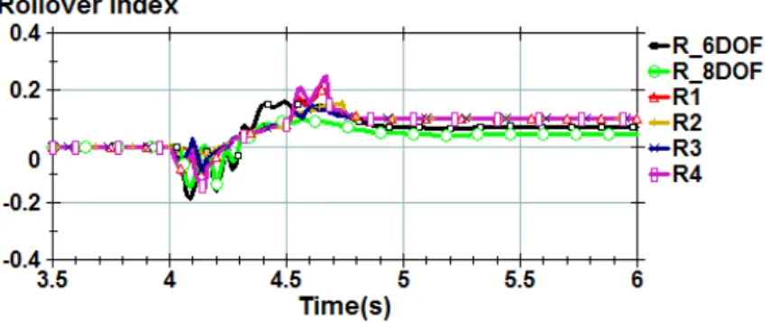
Figure 9: Comparison of the rollover indices: step road input zrl0.15 ,m v 80K m h, 0.

The result of the comparison of the 6 and 8 degrees of freedom indices with all other indices is represented in Figures 10 and 11, respectively.

As can be seen in Figure 11, the indices of the models with 6 and 8 degrees of freedom have better results compared with those in the study (Phanomchoeng & Rajamani, 2013). It can also be said that the model with 8 degrees of freedom has better performance than that with 6 degrees of freedom.

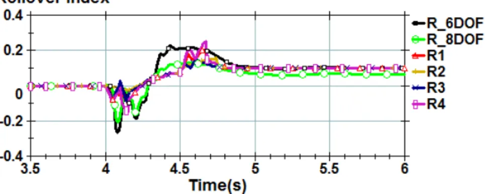
Figure 10: The results of the first test zrl 0.15 ,m  0 for 6 degrees of

freedom model with and comparison with the charts in other studies.

Figure 11: The results of the first test zrl 0.15 ,m  0 for model with

In follownig, two systems with 6 and 8 degrees of freedom are compared with each other and the results obtained in Rajamani studies.

Figure 12: The rollover índices for 6 and 8 degrees of freedom in comparasion with Rajamani index zrl0.15 ,m v 80K m h, 0.

The results of the first test for the state with the added mass equal to zero for 6 and 8 degrees of freedom are displayed in Figure 13.

According to Figure 13, it can be observed that in state without the added mass, diagram of six degrees of freedom quite matches the diagram in the rollover index in the 4 degrees of freedom study and the reference laboratory testing (Phanomchoeng & Rajamani, 2013). The index of 8 de-grees in addition to full compliance, ranging from 4.3 to 4.7 seconds, has better performance com-pared with the final performance of the reference index ((Phanomchoeng & Rajamani, 2013)) and its maximum point is lower. This is extremely helpful to vehicle stability.

Figure 13: Comparison of rollover indices in state without added mass.

Figure 14: The results of the first test for the state without added mass in models with 6 degrees of freedom and comparison with the charts in other studies.

Figure 15: The results of the first test for the state without added mass in models with 8 degree of freedom and comparison with the charts in other studies.

The Fig. 16 indicates the comparision of results of current study with Rajamini previous stud-ies. It is shown that the obtained results are similar with those appeared in Rajamini studstud-ies. The errors that can be seen in Fig. 16 are as the results of ignoring the steering angle in the present study.

In this section, results obtained by applying the second test



zrl 0.15 ,m v 100Km h,



1.2



 _{are presented. All the arguments in the test 1 can be applied}

in the test 2. The results and tables indicated that the stability index is improved in the models with 6 and 8 degrees of freedom presented in this study. According to Figure 17, it can be observed that the model of six degrees of freedom in its rate of maximum reaches the value of 0.3. This is while the final value by Rajamani et al. (Phanomchoeng & Rajamani, 2013) was obtained to be 1. Moreover, in their study, other indicators were observed to have more fluctuations relative to the index with 6 degrees of freedom or greater values compared with the index of 8 degrees of freedom. They had also better performance relative to other indices. Thus, the maximum range of the fluctu-ations of the index is nearly 0.2.

Figure 17: Comparison of rollover indices in second test



zrl 0.15 ,m1.2





.

The results of the second test for the state with the added mass in the models with 6 and 8 de-grees of freedom and in comparison of the charts R4 ((Phanomchoeng & Rajamani, 2013)) can be observed in Figure 18.

According to Figure 18, it can be observed that the indices of the models with 6 and 8 degrees of freedom have better performance compared with indices in other studies. It also can be observed that the model with 8 degrees of freedom has better performance compared with the model with 6 degrees of freedom.

Figure 18: The rollover index in second test



zrl0.15 ,m1.2





for the model with 6 and 8

The results of the second test



zrl 0.15 ,m



1.2



 _{for the state with the added mass equal to}

zero for 6 and 8 degrees of freedom are displayed in Figure 17.

According to Figure 19, results in the state with the added mass equal to zero in the charts with 6 and 8 degrees of freedom confirm the accuracy of the indices and in addition, approve that the charts have better performance relative to the R4 in the study (Phanomchoeng & Rajamani, 2013). Considering the steering angle results in the appropriate compatibility between the Rajamani calculated rollover index with those achieved in the present study.

Figure 19: the results of second test for the state without added mass in the models with 6 and 8 degrees of freedom and in comparison with the R4 (Phanomchoeng & Rajamani, 2013).

5 CONCLUSIONS

In this paper, new rollover indices for the models with 6 and 8 degrees of freedom were respectively presented as improved versions of the models with 4 degrees of freedom. The new presented indices were compared with the existing models with 4 degrees of freedom in other studies. This compari-son was conducted in the Carsim software as a powerful application for simulation of vehicle sys-tems. After simulation of the three systems of 4, 6, and 8 degrees of freedom in this software and through specific tests according to the scientific findings ((Phanomchoeng & Rajamani, 2013)), im-provement in the new stability indices was observed. The good performance of the new system can be easily seen in the first and second tests. The performance improvement in the new systems is high in the moment the tire is detached from the ground surface. This was low in the old system so that the automobile was in the threshold to rollover. In the new model, the stability is in the state when tires are slightly detached from the ground surface. In the first test, the index was obtained about 20% less than other indices. In the second test, the value increased to 60% for the model with 6 degrees of freedom and to 80% for the model with 8 degrees of freedom. It was also specified that the automobile had better stability performance in the 8 degrees of freedom model compared with the 6 and 4 degrees of freedom models.

References

Ahmadian, Mehdi. (2014). Integrating Electromechanical Systems in Commercial Vehicles for Improved Handling, Stability, and Comfort. SAE International Journal of Commercial Vehicles, 7(2014-01-2408), 535-587.

Chen, Bo-Chiuan, & Peng, Huei. (1999). A real-time rollover threat index for sports utility vehicles. Paper presented at the American Control Conference, 1999. Proceedings of the 1999.

Dilich, MA, & John, M Goebelbecker. (1997). Truck rollover. Safety Bulletin, Triodyne Inc, 6(1).

Hsu, Ling-Yuan, & Chen, Tsung-Lin. (2012). Vehicle dynamic prediction systems with on-line identification of vehi-cle parameters and road conditions. Sensors, 12(11), 15778-15800.

Johansson, Björn, & Gafvert, Magnus. (2004). Untripped SUV rollover detection and prevention. Paper presented at the Decision and Control, 2004. CDC. 43rd IEEE Conference on.

Kong, YS, Abdullah, SHAHRUM, Omar, MOHD ZAIDI, & Haris, SALLEHUDDIN MOHAMED. (2016). Topologi-cal and topographiTopologi-cal optimization of automotive spring lower seat. Latin American Journal of Solids and Structures, 13(7), 1388-1405.

National Highway Traffic and Safety Board, Traffic safety facts. (2011). http://www.safercar.gov/Vehicle+Shoppers/Rollover/Fatalities.

Odenthal, Dirk, Bunte, Tilman, & Ackermann, Jurgen. (1999). Nonlinear steering and braking control for vehicle rollover avoidance. Paper presented at the Control Conference (ECC), 1999 European.

Pagnacco, Emmanuel, Zidani, Hafid, Sampaio, Rubens, de Cursi, Eduardo Souza, & Ellaia, Rachid. (2016). Design Optimization of a Random Suspension Device Considering a Reliability Constraint on the Frequency Response Func-tion. Latin American Journal of Solids & Structures, 13(6).

Pan, Qiang, He, Tian, Xiao, Denghong, & Liu, Xiandong. (2016). Design and Damping Analysis of a New Eddy Current Damper for Aerospace Applications. Latin American Journal of Solids and Structures, 13(11), 1997-2011. Peters, Steven Conrad. (2006). Modeling, analysis, and measurement of passenger vehicle stability. Massachusetts Institute of Technology.

Phanomchoeng, Gridsada, & Rajamani, Rajesh. (2012). Prediction and Prevention of Tripped Rollovers. Intelligent Transportation Systems Institute Center for Transportation Studies University of Minnesota.

Phanomchoeng, Gridsada, & Rajamani, Rajesh. (2013). New rollover index for the detection of tripped and un-tripped rollovers. IEEE Transactions on Industrial Electronics, 60(10), 4726-4736.

Rajamani, R, Piyabongkarn, D, Tsourapas, V, & Lew, JY. (2009). Real-time estimation of roll angle and CG height for active rollover prevention applications. Paper presented at the 2009 American control conference.

Rajamani, Rajesh. (2011). Vehicle dynamics and control: Springer Science & Business Media.

Rajamani, Rajesh, & Phanomchoeng, Gridsada. (2013). New rollover index for the detection of tripped and un-tripped rollovers. IEEE Transactions on Industrial Electronics, 60(10), 4726-4736.

Solmaz, Selim, Corless, Martin, & Shorten, Robert. (2006). A methodology for the design of robust rollover preven-tion controllers for automotive vehicles: Part 1-Differential Braking. Paper presented at the Proceedings of the 45th IEEE Conference on Decision and Control.

Solmaz, Selim, Corless, Martin, & Shorten, Robert. (2007). A methodology for the design of robust rollover preven-tion controllers for automotive vehicles with active steering. Internapreven-tional Journal of Control, 80(11), 1763-1779. Solmaz, Selim, Shorten, Robert, Wulff, Kai, & Cairbre, Fiacre O. (2008). A design methodology for switched discrete time linear systems with applications to automotive roll dynamics control. Automatica, 44(9), 2358-2363.

Tavan, Nematollah, Tavan, Mehdi, & Hosseini, Rana. (2015). An optimal integrated longitudinal and lateral dynam-ic controller development for vehdynam-icle path tracking. Latin Amerdynam-ican Journal of Solids and Structures, 12(6), 1006-1023.