Abstract
In this paper, dynamic material constants of 2-parameter Mooney-Rivlin model for elastomeric components are identified in broad frequency range. To consider more practical case, an elastomeric engine mount is used as the case study. Finite ele-ment model updating technique using Radial Basis Function neural networks is implemented to predict the dynamic material constants. Material constants of 2-parameter Mooney-Rivlin model are obtained by curve fitting on uni-axial stress-strain curve. The initial estimations of the material constants are achieved by using uni-axial tension test data. To ensure of the consistency of dynamic response of a real component, frequency response function of three similar engine mounts are extracted from experimental modal data and average of them used in the procedure. The results showed that this technique can success-fully predict dynamic material constants of Mooney-Rivlin mod-el for mod-elastomeric components.
Keywords
Mooney-Rivlin model, Dynamic Material Constants, Frequency response function, Radial Basis Function Neural Networks, Elas-tomeric components
Predicting the dynamic material constants
of Mooney-Rivlin model in broad frequency
range for elastomeric components
1 INTRODUCTION
Elastomeric materials are widely used in noise and vibration isolation mechanisms at different in-dustries such as automotive, aerospace, building and so on. Substantial improvement in isolator performance requires the construction of large quantity of samples and experimental tests that is very time consuming process. Proper use of finite element models can reduce the number of samples and experimental tests. Comparing metallic components, the mechanical properties of elastomers
Kam al Jahani a
H ossein M ahm oodzade b
a Mechanical Engineering Department,
University of Tabriz , 29th Bahman Blvd., 51666-16471, Tabriz, Iran (phone: +98 411 3393044; fax: +98 411 3354153;
b Mechanical Engineering Department,
Latin American Journal of Solids and Structures 11 (2014) 1983-1998
are not well known and depend on many ambient and working conditions such as temperature, frequency and dynamic amplitude, etc (Rendek and Lion, 2010, Hofer and Lion, 2009). Therefore, using appropriate models for elastomers with proper material constants to achieve more realistic and accurate results is crucial in any finite element code. There exist some constitutive models (such as Mooney-Rivlin, Ogden, Neo-Hookean, Polynomial Form, Arruda-Boyce, Yeoh,…) that can simulate hyperelastic behavior of the elastomers. The Mooney-Rivlin constitutive model will be discussed in more details in this paper.
Usually elastomeric components experience both shock loads (that exert large deformations on the elastomer in low frequency) and vibration loads (that excite the component in low amplitude deformation and high frequency). In most of the published works, the static (or low frequency) ten-sion /or compresten-sion tests have been conducted on the samples and using curve-fitting techniques, the material constants of Mooney-Rivlin model have been extracted. Guo and Sluys (2006) dis-cussed different static tension test methods to extract the material constants and used these results to verify their proposed constitutive model. Cristopherson and Jazar (2006) used Mooney-Rivlin model in FE modeling of a passive hydraulic engine mount and determined the Mooney-Rivlin con-stants by curve fitting on uniaxial experimental stress-strain data. Khalilollahi et al. (2002) investi-gated the static behavior of elastic materials using Mooney-Rivlin model. The material coefficients of the model were achieved using experimental tests. Silva and Bittencourt (2008) used Mooney-Rivlin hyperelastic model in shape optimization of elastomeric media of an engine mount. Pereira and Bittencourt (2010) used the 2 parameter Mooney-Rivlin constitutive model in topological sen-sitivity analysis. Pearson and Pickering (2001) obtained the constants of Mooney-Rivlin model us-ing axial tensile test and showed that usus-ing these constants, the static behavior of the elastomeric material is predicted well. Korochkina et al. (2008) investigated the applicability of various consti-tutive models to predict the nonlinear stress–strain behavior of silicone rubber pads. To determine the material parameters, they used uni-axial tension and pure shear test data. The material param-eters were determined through a least-squares-fit procedure, which minimizes the relative error in stress.
To determine the dynamic mechanical characteristics of elastomers, in most of the documented methods the elastic and storage moduli (or elastic modulus and loss factor) have been used as mate-rial properties where, these properties extracted from resonant tests (Gupta et al., 1999, Jahani and Nobari, 2010, Wismer and Gade, 1997). However, there are a few publications about dynamic mate-rial constants of the hyperelastic models for elastomers at broad frequency range. For instance, Kim et al. (2004) formulated a new constitutive model by using Mooney-Rivlin constants to predict the dynamic characteristic of rubbers superimposed to large static deformation but, they only presented results for frequencies below 30 Hz.
Latin American Journal of Solids and Structures 11 (2014) 1983-1998
2 EXPERIMENTS AND TEST SAMPLES
2.1 Samples
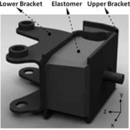
To consider a more practical case in the present work, an elastomeric engine mount is investigated that is illustrated in Figure 1. The component includes upper and lower steel brackets and elasto-meric media in the middle. The engine mount is a flat type and elastoelasto-meric media approximately has cubic shape.
Figure 1:Investigated elastomeric engine mount.
2.2 Tests
2.2.1 Tension Test
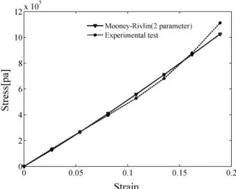
To obtain Mooney-Rivlin constants, present method rely only on the 3-D FE model of the elasto-meric sample and experimental FRF(Frequency response function) data and is independent of ex-perimental stress-strain curves , however to have initial estimation of Mooney-Rivlin constants, the sample was stretched in the vertical direction(z-direction). Using the graph of stress-strain obtained from tension test and implementing curve fitting, the initial static coefficients of the material model were obtained. A schematic of tensile test rig is presented in Figure 2. The stress-strain graph of the investigated sample and curve fitted graph have been shown in Figure 3. Mooney-Rivlin material constants for the investigated engine mount that extracted from curve fitting procedure are: c!"! =2621676 and c!"! =−1851093 (brief explanations of these material constants are presented
Latin American Journal of Solids and Structures 11 (2014) 1983-1998 Figure 2: Schematic of tensile test rig.
Figure 3:The stress-strain graph of the sample and fitted graph.
2.2.2 Modal tests of the samples
Experimental FRF data of the engine mount is obtained by impact hammer test and modal analy-sis. A schematic of the modal test train is presented in Figure 4. Specifications of Test tools and instruments used in this study are presented in Table 1. Tests are done in vertical or z- direction in free-free condition. Atmospheric conditions of the lab during the tests were as following: Relative humidity=50%; Temperature=26°C. In order to ensure of the reliability and repeatability of the test results, 3 similar samples are tested. For instance, FRFs of the samples in z-direction are plot-ted with together in Figure 5. The natural frequencies of three samples are presenplot-ted In Table 2.
Item Mark and Type Data logger and signal analyzer unit B&K 2035
Impact hammer B&K 8202 Accelerometer B&K 4395 Tension test machine MTS
Latin American Journal of Solids and Structures 11 (2014) 1983-1998 Natural Frequency (Hz)
Sample1 Sample2 Sample3 212 193 192 394 381 379 576 576 570 762 702 691
Table 2: Natural frequencies of the engine mounts in vertical (z) direction in free-free condition.
Figure 4:Schematic of Modal test train.
Latin American Journal of Solids and Structures 11 (2014) 1983-1998
2.2.3 Modal test of metallic parts of the sample.
Each of the samples has two metallic parts namely lower bracket assembly and upper bracket as-sembly. For the purpose of model updating task (see section 3.1.), the brackets of one of the inves-tigated engine mounts separated from elastomeric part and cleaned then FRFs of these metallic parts are obtained using impact hammer test in free-free condition. In Table 3, the natural fre-quencies of the brackets are presented.
Natural frequencies [Hz]
z- direction y-direction Upper bracket 540 -
Lower bracket 636 293 504
Table 3: Natural frequencies of the investigated engine mount's brackets in z-direction. .
3 FE MODEL
The brackets are modeled using shell elements (shell 281) and elastomeric media is modeled using 3-D solid elements (8 nodes brick elements namely solid185) and 2- parameter Mooney-Rivlin model is selected as the material model in Ansys software. FE model of the sample is illustrated in Figure 6.
Figure 6:FE model of the sample.
3.1 Model updating of metal parts of the engine mounting
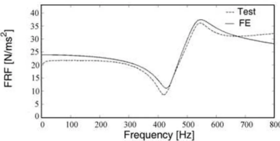
ob-Latin American Journal of Solids and Structures 11 (2014) 1983-1998 tained through model updating processes. At first, the experimental FRFs of the metal parts are obtained by implementing impact hammer test. Then it is tried to identify the material properties of the components to give the best correlation between the FRFs obtained from the test and FE models. For example, the experimental and updated FE FRFs of upper bracket in z-direction are illustrated in Figure 7. The updated material properties for the brackets are presented in Table 4.
Young' modulus
[GPa] Poisson's ratio
Mass density [kg/mm!]
Upper bracket 208 0.29 7800 Lower bracket 220 0.29 7800
Table 4: Updated material properties of the brackets.
Figure 7:FRFs of updated FE model and test for upper bracket.
3.2.Mooney-Rivlin material model
Mooney–Rivlin material model that describe the rubber like materials behavior, has the variants of 2, 3, 5, and 9 terms material constants (Mooney, 1940, Rivlin, 1948). The strain energy potential function, E, of an isotropic material is customarily formulated in terms of three invariants of the stretch ratios. These are generally taken to be the principle invariants, I1, I2 and I3 of the right Cauchy-Green deformation tensor (Blatz et.al, 1973). The strain energy potential functions are usu-ally assumed to have polynomial or reduced polynomial forms. Considering Mooney-Rivlin material models, the polynomial form for an incompressible elastomeric material can be expressed as follow-ing:
E
=
Cij
(
I
1!3)
i(
I
2!
3)
ji+j=1 N
"
(1)Where
I
1=
!
1 2+
!
22
+
!
32
I
2=
!
1 2!
2 2+
!
22
!
32
+
!
12
!
32
λ1 and λ2are the principal stretches.
Latin American Journal of Solids and Structures 11 (2014) 1983-1998
I
3=
!
1 2!
2 2!
3 2=
1
Depending on the value of N, different variants of Mooney-Rivlin model will be formed. For exam-ple, N=3 constructs 9-parameter Mooney-Rivlin model (the material parameters are c01, c10, c11, c02, c20, c21, c12, c30, c03) and N=1 stands for 2-parameter Mooney-Rivlin model. In later case, considering Eqn.1, the strain energy potential function is expressed as following
E
=
C
10
(
I
1!
3)
+
C
01(
I
2!
3)
(2) Where, c10, c01 are the material constants.3.3 Studying the static performance of the sample
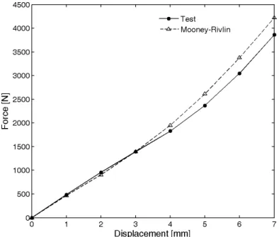
To ensure that the elastomeric engine mount is modeled correctly and the static coefficient of Mooney-Rivlin material model is estimated properly, first the static performance of the sample is investigated. The results of static analysis with together the experimental results that was achieved in section 2.2.1, are presented in Figure 8. This figure shows that the prediction of the static be-havior of the component is acceptable.
Figure 8:Comparing force-displacement curves of the static test and FE analysis for the investigated component.
4 RADIAL BASES FUNCTION NEURAL NETWORKS
Latin American Journal of Solids and Structures 11 (2014) 1983-1998 Figure 9:Architecture of a radial basis function neural network.
The overall response characteristic of an RBFN is presented in Eqn. (3) (More details can be found in (Atalla and Inman, 1998).
f
i=
b
j+
W
i j!
(
{ }
x
!
c
i
{ }
,
sc
)
i=1
n
"
(3)Where,
{ }
x
is the value of input vector,c
i{ }
is the center of the ith RBF neuron, sc is the spreadconstant of the network (the same for every neuron), represents the Euclidean norm
(2-norm).φ
!
is the radial basis function of the network (the same for every neuron) ,f
i f! is the output of the jth linear neuron andw
ij is the weight between the ith RBF neuron and jth linearneuron and n is the number of RBF neurons.
There are two types of data that can be used for identification of dynamic characteristics of an elastomeric component, namely FRF data and Modal data. In the present work, the FRF data will be implemented.
The RBFN is trained with data obtained from solving the direct problem N times where, N is the number of training sets. To train an RBFNN, it is necessary to set every network parameter, i.e., every RBF center, all the weights and biases of the linear neuron and the spread constant. The centers of an RBFNN should be spread out over the range of the input space occupied by the input vectors. In the present work all of the input vectors are chosen as centers.
Training a RBFNN comprises the following steps:
1- The distance between each column of the input matrix X and each neuron in the hidden layer
(represented by its centre c) is measured, resulting in the matrix D of distances. The element d !" of
Latin American Journal of Solids and Structures 11 (2014) 1983-1998
2- The output of the hidden layer is calculated by.
h
j,i=
e
!dj,i/scThe elements of H, which
measure how much the ith input vector resembles the centre of the jth neuron, range between zero and one.
3- The network output Y is calculated by a linear combination of the elements of H,
Y
=
W
*
H
(4)Training a RBFNN, means finding the weight matrix W the only unknown of the problem. Solv-ing the equation above for W yields
*
W
=
Y
H
+ (5)Where
H
+is the pseudo-inverse of H. Once it has been trained, the network can be used to
estimate model parameters based on new input vectors.
4- The network generalization characteristics should be verified before implementing it. Generaliza-tion is the behavior of the network output when presented with an input vector not used to train the network.
5 IDENTIFICATION OF THE MATERIAL CONSTANTS OF THE MOONEY-RIVLIN
MODEL IN LOW AMPLITUDE HIGH FREQUENCY RANGE
Here, it is tried to identify the material coefficients (
c
10,
c
01 ) using FRF data. Identification pro-cess is conducted using RBFNN. The training sets of the RBFNN consist of sensitive bands of FRFs (frequency bands around peaks) as inputs and material constants coefficients as targets. Usu-ally, elastomers show frequency and amplitude dependent behavior and in most cases the stiffness of elastomers will increase with increasing the frequencies. So here, to generate input FRFs, the mate-rial properties are changed gradually (from the values derived from static tension test until the twice of them) as Eqn. 6.c
10=
c
100
(1
+
0.1
!
!
) &
c
01
=
c
010
(1
+
0.1
!
!
),
!
=
0,1,...,
N
(6)Where, c!"! and c!"! are the material constants that derived from static tension test.
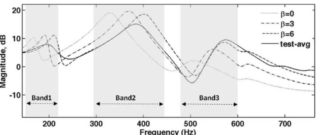
Latin American Journal of Solids and Structures 11 (2014) 1983-1998 Figure 10:FRFs that are achieved from three different values of β are compared with the test counterpart.
Appropriate RBFNN for each of the frequency bands is constructed using resonant frequencies. For example training sets for the Band2 is presented in Table 5. Many points of a FRF graphs in each frequency band can be used in identification process using artificial neural networks. Even though this strategy may lead to more accurate identified values however, it also needs many training sets. Location of Table 5.
After training the corresponding RBFNN of a specified frequency band, the measured frequency response function (here the resonant frequency) in the same frequency band is fed to the network and value of corresponding β is determined. Then using equation 6, the material constants of the 2-parameter Mooney-Rivlin model, namely c!" and c!", are identified. The flowchart of the identifi-cation process is illustrated in Figure 11. The predicted material constants using this procedure for the investigated engine mount is presented in Figure 12. Also using these predicted material con-stants in z-direction, the stress-strain curves at different frequencies are plotted in Figure 13. Con-sidering these results, it is evident that the elastomeric component shows frequency dependent be-havior and also, there is deviation from isotropic assumption in a real elastomeric component.
Training set / No. 1 2 3 4 Input: Resonant frequency
328 369 391 402
Target: β 0 3 5 6
Latin American Journal of Solids and Structures 11 (2014) 1983-1998
Figure 11:Flowchart of the identification procedure.
Latin American Journal of Solids and Structures 11 (2014) 1983-1998 Figure 13:Stress-strain diagram at different frequencies in z- direction for the investigated engine mount.
6 IDENTIFICATION OF THE MATERIAL CONSTANTS OF THE MOONEY-RIVLIN
MODEL IN HIGH AMPLITUDE LOW FREQUENCY RANGE
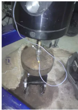
Here, in order to investigate the effect of deflection amplitude on the coefficients of 2-parameter Mooney-Rivlin model, a new test setup is implemented in low frequency range. This test setup is shown in Figure 13. In current setup, different weights (namely with masses of 2.5, 7.5 and 25 kg) are added on the top of engine mount and the mount is fixed from the bottom brackets to a heavy rigid block. It is obvious that this kind of boundary condition allows moderate deflection of the sample comparing to the low deflection in Free-Free condition. Addition of weight on the sample extremely reduces the natural frequencies of the system. For instance, time response on the top of the engine mount using 2.5Kg weight is presented in Figure 14.
Latin American Journal of Solids and Structures 11 (2014) 1983-1998 Figure 13:Low-Frequency test setup.
Latin American Journal of Solids and Structures 11 (2014) 1983-1998 Figure 15: Predicted material constants of the 2-parameter Mooney-Rivlin model for elastomeric media of the
elas-tomeric engine mount, c!" in: ______ low-frequency range and - - - - High-frequency range.
Figure 16:Predicted material constants of the 2-parameter Mooney-Rivlin model for elastomeric media of the elastomeric engine mount, c!" in: ______ low-frequency range and - - - - High-frequency range.
7 CONCLUSION
Latin American Journal of Solids and Structures 11 (2014) 1983-1998
procedure is general and can be applied to identify dynamic material constants of the other consti-tutive models such as Ogden, Neo-Hookean, etc for elastomers.
References
Atalla, M.J, Inman, D.J. (1998). On Model Updating Using Neural Networks. Mechanical Systems and Signal Pro-cessing.
12: 135-161.
Blatz, P.J., Sharda, S.C., Tschoegl, N.W. (1973). A new elastic potential function for rubbery material. Proceedings of the National Academy of Sciences of the United States of America 70: 3041–3042.
Christopherson, J., Jazar, G.N. (2006). Dynamic behavior comparison of passive hydraulic engine mounts: Part 2Finite element analysis. Journal of Sound and Vibration 290: 1071-1090.
Guo Z., Sluys, L.J. (2006). Application of a new constitutive model for the description of rubber-like materials under monotonic loading. International Journal of Solids and Structures 43:2799-2819.
Gupta, A., Khandaswamy, S., Yellepeddi, S., Mulcahy, T., Hull, J. (1999). Dynamic modulus estimation and struc-tural vibration analysis. Proceedings of the 17th International Modal Analysis Conference, Kissimmee FL(UA) Proc SPIE 3727: 1423–1427.
Hofer,P. ,Lion, A. (2009). Modelling of frequency- and amplitude-dependent material properties of filler-reinforced rubber. Journal of the Mechanics and Physics of Solids 57:500-520.
Jahani, K., Nobari, A.S. (2010). Identification of damping and dynamic young’s modulus of a structural adhesive using radial basis function neural networks and modal data. Experimental Mechanics 50:607–619.
Khalilollahi, A, Felker, B.P., Wetzel, J.W. (2002). Non-linear elastomeric spring design using Mooney-Rivlin con-stants, Proceedings of 2002 ANSYS Users Conference and Exhibition, Paper.146.
Kim, B.K., Youn, S.K., Lee, W.S. (2004). A constitutive model and FEA of rubber under small oscillatory load superimposed on large static deformation, Archive of Applied Mechanics 73:781–798.
Korochkina, T.V., Jewell, E.H., Claypole, T.C., Gethin, D.T. (2008). Experimental and numerical investigation into nonlinear deformation of silicone rubber pads during ink transfer process, Polymer Testing 27 : 778-791.
Mooney, M. (1940). A theory of large elastic deformation, Journal of Applied Physics 11:582-592.
Pearson, I., Pickering, M. (2001).The determination of a highly elastic adhesive's material properties and their repre-sentation in finite element analysis, Finite Elements in Analysis and Design 37: 221-232.
Pereira, C.E.L. and Bittencourt, M.L. (2010). Topological sensitivity analysis for a two-parameter Mooney-Rivlin hyperelastic constitutive model, Latin American Journal of Solids and Structures 7:391-411.
Rendek, M., Lion, A. (2010). Amplitude dependence of filler-reinforced rubber: Experiments, constitutive modelling and FEM – Implementation, International Journal of Solids and Structures 47: 2918–2936.
Rivlin, R.S. (1948). Large elastic deformations of isotropic materials. IV. Further developments of the general theory, Philosophical Transactions A 241:379-397.
Silva, C.A.C. and Bittencourt, M.L. (2008). Structural shape optimization of 3D nearly-incompressible hyperelastici-ty problems, Latin American Journal of Solids and Structures 5:129-156.