Abstract
The objective of this paper is representation of an analytical solu-tion to calculate transmission loss (TL) of an arbitrarily thick cylindrically orthotropic shell, immersed in a fluid medium with a uniform external airflow and contains internal fluids. The shell is assumed to be infinitely long and is excited by an oblique plane wave. The displacements are expanded as cubic functions of the thickness coordinate to present an analytical solution based on Third-order Shear Deformation Theory (TSDT). Equations of motion of the shell are then obtained using virtual work method. By solving shell vibration as well as acoustic wave equations sim-ultaneously, the exact solution for TL is obtained. Predictions with the presented models are compared with those of previous models (CST and FSDT) for thin shells. Similar results are achieved as the effects of shear and rotation on TL are not notice-able in a thin shell. However, the model introduced here exhibits more accurate results for thick shells where the shear and rotation effects become more significant in lower R/h ratios. Additionally, the effects of related parameters on TL such as material and geo-metrical properties are discussed.
Keywords
Orthotropic shells, Transmission loss, Third order shear defor-mation theory, Acoustic.
Sound Transmission across Orthotropic Cylindrical Shells Using
Third-order Shear Deformation Theory
M. H. Shojaeefard 1 a R. Talebitooti 2 b,c R. Ahmadi 3 d M. R.Gheibi 4 e
a Prof., Sch. of Mech. Eng., Iran Univ. of Sci. and Tech., Iran, [email protected]
b Asst. Prof., Sch. of Mech. Eng., Iran Univ. of Sci. and Tech., Iran, [email protected]. c Automotive Simulation & Optimal Design Research Lab., Sch. of Auto. Eng., Iran Univ. of Sci. and Tech., Tehran, Iran.
Latin American Journal of Solids and Structures 11 (2014) 2039-2072 Nomenclature
3, 1
c c Speed of sound in external and cavity medium TL Transmission Loss
E Module of elasticity (u u u1, ,2 3) Displacements of a point on the plane h3 =0
r
f Ring frequency V Velocity of the external flow
c
f Critical frequency I
W Incident power flow per unit length
G Shear stiffness T
W Transmitted power flow per unit length
h Shell wall thickness a Incident angle
1 n
H Cylindrical Henkel functions of the first kind of
integer order n amax,amin Critical angles of incidence
2 n
H Cylindrical Henkel functions of the second kind
of integer order n dK Virtual kinetic energy
n
I Mass inertia dU Virtual strain energy
n
J Cylindrical Bessel function of the first kind of
order n dV Virtual potential energy
k Wave number en Neumann factor
,
r z
k k Wave numbers in h3and h1 direction (h h h1, ,2 3) Displacements of the shell in the radial,
cir-cumferential and axial directions
1
M Mach number u Poisson’s ratio
n Circumferential mode number w Angular frequency
0
P Amplitude of the incident wave r Mass density of shell per unit mid-surface area
1 I
P Acoustic pressures of the incident wave r r3, 1 Density of external and internal medium
1R
P Acoustic pressures of the reflected wave sij Stress components
3T
P Acoustic pressure of the transmitted wave tij Strain (shear strain) components
i
q Transverse load on the surface of the shell t Average power transmission coefficient
ij
Q Orthotropic reduced stiffness coefficients fi Rotations of transverse normal on plane h3=0
R Radii of cylinder Laplacian operator
Latin American Journal of Solids and Structures 11 (2014) 2039-2072 1 INTRODUCTION
Acoustic transmission is investigated in this study through an arbitrarily thick orthotropic cylinder of infinite length, which is excited by a diffuse field. This issue has been addressed in the literatures to a large extent. Several attempts have performed significant studies on isotropic, orthotropic and laminated fiber-reinforced composite shells. Smith (1957) developed a theoretical study in isotropic cylindrical shells taking into account inward-traveling wave as an only parameter. TL was then introduced by the same author as the ratio of absorbed power to incident power per unit length. White (1966) analyzed sound transmission into finite cylindrical shells and obtained two important characteristics, namely ring frequency and coincidence frequency, with maximum values of the ob-tained TL. Koval (1976 and 1979) utilized displacement field of Nelson et al. (1958) to show math-ematical models for estimation of the TL of oblique plane sound waves through an orthotropic infi-nite shell. The effects of membrane and bending were considered as well, though transverse shearing and rotational inertia were not taken into account. The effect of orthotropic behavior on TL was parametrically studied for the shell’s elastic properties along circumferential and axial directions. The main feature of his contribution was considering external airflow, external plane wave with an incident angle and internal pressure of the cylindrical shell. Transmission of airborne noise was studied by this solution through isotropic and orthotropic fuselage under flight conditions using impedance method. An analytical model was suggested by Koval (1980) for predicting TL of lami-nated composite infinite cylindrical shells excited by an oblique plane wave. Transverse shearing and rotational inertia were not considered in this research work. Blaise et al. (1991) extended Ko-val’s (1979) work and followed an orthotropic shell excited by an oblique plane sound wave with two independent incident angles for calculation of the diffuse field transmission coefficient. They compared the numerical results with Koval’s results and found some numerical errors in his work. In their study, they used a Donnell–Mushtari's displacements field for orthotropic cylinders ignoring transverse shearing and rotational inertia. Diffuse field transmission coefficient was calculated based on two independent incident angles. Moreover, they extended definition of the ring and critical fre-quencies to an infinite orthotropic shell excited by a plane wave. Furthermore, a model was devel-oped for acoustic transmission of the oblique incidence of multi-layered cylindrical shells (Blaise et al., 1992). Finally, the same authors presented a new model taking into account 3D displacement fields in thickness for the acoustic transmission through an orthotropic multi-layered infinite cylin-drical shell (Blaise et al., 1994). Tang et al. (1996) studied sound transmission through infinite cy-lindrical sandwich shells illuminated an oblique plane wave with two different incident angles. They presumed same Blaise's assumptions for incident angles and acoustic media. The effects of external airflow and pressure difference between inside and outside shell surfaces were considered in their study for different fluids in both sides of the shell. They utilized first order shell theory for thick shells to calculate the TL.
Latin American Journal of Solids and Structures 11 (2014) 2039-2072
two models for calculating diffuse field transmission into composite laminate and sandwich compo-site infinite cylinders. They considered membrane, bending, transverse shearing as well as rotational inertia effects and orthotropic ply angle of the layers in both models.
Classical shell theory (CST) was utilized in most of the above citations to model the shell vibra-tion. However, it cannot be used for thick shells and even thin shells when the number of circumfer-ential waves increases as the result of neglecting shear deformation and rotary inertia effects in CST. Implementation of CST for thick and relatively thick shells can cause significant errors in such cases. An exact solution was found by Daneshjou et al. (2007, 2008 and 2009) more recently in a series form based on CST and first order shear deformation theory (FSDT). They considered all three displacements of the shell for orthotropic and laminated composite cylindrical shells. They also showed that considering the effects of shear and rotation in FSDT for thin shells leads to re-duction of TL in high frequency range in comparison with CST. Just recently, Daneshjou et al. (2010) proposed an improved model for sound transmission through relatively thick FGM cylindri-cal shells based on third order shear deformation theory (TSDT). In addition, they have shown that for relatively thick FGM shells where the shear and rotation effects become more significant in
low-er R/h ratio, TSDT presents more accurate results.
The existing literature lacks a comprehensive work on sound transmission of thick orthotropic cylindrical shells. In order to modify previous studies, noting that the best presented model in liter-ature can not include the proper modeling for thick shells due to its assumptions on the straightness and normality of transverse normal during deformation. Therefore, in this paper it has been tried to use third order shear deformation theory (TSDT) which relaxes these assumptions by expanding the displacements as cubic functions of the thickness coordinate. Thus, this paper presents a novel and accurate modeling of the acoustic transmission of a thick-wall orthotropic cylindrical shell with subsonic external flow based on TSDT. Then, the obtained results are compared with those availa-ble in the literature. The comparison reveals a good agreement. This paper also intends to quantify the effects of orthotropic cylindrical shell characteristics on TL. At last, the numerical results are used to address the effects of geometrical properties and material properties.
2 STATEMENT OF THE PROBLEM
Figure 1 depicts an orthotropic cylindrical shell of infinite length, radius,R, wall thickness,h and
mass density of shell per unit mid-surface area,
r
, which is irradiated to an oblique plane wave withthe incident angle of a from outside. A uniform external airflow at velocity V in the exterior fluid
medium impinges on the shell. Moreover, ri and ci with subscripts 1 and 3 are used respectively
to introduce external and internal density and also the speed of acoustic media. Also, the interior side of the shell is assumed to be anechoic, which means that only inward-traveling wave exists. As
shown in the Figure 1, (h h h1, 2, 3) denote the orthogonal curvilinear coordinate system where the
1
h is coincident with the axis of cylindrical shell, while h2 and h3 are circumferential and
Latin American Journal of Solids and Structures 11 (2014) 2039-2072
Figure 1: Schematic diagram of the cylindrical shell
3 THEORITICAL FORMULATIONS
Particular assumptions are considered in developing a thick shell theory as follows (Reddy, 2003):
(1) The transverse normal is inextensible (i.e. e33 = 0).
(2) There is no reason for straightness and normality of a transverse normal during deformation. (3) The transverse normal stress is negligible in order that the plane stress assumption cannot be considered.
These assumptions will be used in formulation of the problem.
3.1 Kinematic relations
For the cylindrical shells, the strain-displacement relation can be presented as (Qatu, 2004):
1 2 3
11 22 3 33
1 3 2 3
1
; ;
1
U U U
U R
R
e e e
h h h h
é ù
¶ ê¶ ú 
= = ê + ú =
æ ö
¶ ç ÷ ë¶ û 
÷ +
ç ÷
ç ÷
çè ø
3 2
12 1
3 2 1 3
1
1
1 1
U
U R
R
R R
R R
h e
h h h h
æ ö÷
ç ÷
ç ÷
ç
æ ö ÷
¶ ç ÷÷ ¶ çç ÷÷
= æ ö + ççç + ÷÷ çç æ ö÷÷
¶ è ø¶ ç ÷
÷ ÷
ç + ÷ ç ç + ÷÷
ç ÷ ç ç ÷÷
ç ÷ ç ÷÷÷
ç ç ç
è ø è è øø
1 3 3 2 3
13 23
3 1 3 3 3 2
1
; 1
1 1
U U U U
R R
R R
R R
h
e e
h h h h h h
æ ö÷
ç ÷
ç ÷
ç
æ ö ÷
¶ ¶ ç ÷÷ ¶ çç ÷÷ 
= + = ççç + ÷÷ çç æ ö÷÷+ æ ö
¶ ¶ è ø¶ ç çç çè èçç çç + ÷øø÷÷÷÷÷÷÷÷ çççèç + ÷÷÷÷ø 
Latin American Journal of Solids and Structures 11 (2014) 2039-2072
where
R
is the radii of cylinder and (U U U1, 2, 3) represent the shell displacements along (h h h1, 2, 3) coordinates. It should be mentioned the only assumption made here is the small displacements. No other assumptions are considered in this formulation.3.2 Stress – strain relations
The stress-strain relations for an orthotropic cylindrical shell can be presented by the Hook’s law as (Chakrabartiet al., 2013):
11 11 12 11
22 21 22 22
12 66 12
13 55 13
23 44 23
0 0 0
0 0 0
0 0 0 0
0 0 0 0
0 0 0 0
Q Q
Q Q
Q Q
Q
s e
s e
s e
s e
s e
ì ü é ù ì ü
ï ï ï ï
ï ï ê úï ï
ï ï ê úï ï
ï ï ï ï
ï ï ê úï ï
ï ï ï ï
ï ï ê úï ï
ï ï= ï ï
í ý ê úí ý
ï ï ê úï ï
ï ï ï ï
ï ï ê úï ï
ï ï ï ï
ï ï ê úï ï
ï ï ê úï ï
ï ï ï ï
ï ï ï ï
î þ ë û î þ
(2)
where
s
ij ande
ij denote stress and strain components in the orthotropic layer andQ
ij, denotesthe in-plane-stress reduced stiffness constants that are defined in terms of material properties of the orthotropic ply, which can be defined as:
1 12 2 2
11 12 22
12 21 12 21 12 21
; ;
1 1 1
E E E
Q Q n Q
n n n n n n
= = =
- -
-44 23 ; 55 13 ; 66 12
Q =G Q =G Q =G
(3)
where E11 and E22 are respectively the module of elasticity in h1 and h2 directions, while G23,
13
G and G12 are the modules of rigidity and u12 and u21 represent the Poisson’s ratios.
Relaxing the straightness and normality of a transverse normal during deformation, the dis-placement field for third-order shear deformation theory represented as (Lee and Reddy, 2004, Chakrabarti, 2013):
(
)
(
)
(
)
3 31 1 2 3 1 1 2 3 1 1 2 1 3 1
1
, , , , , , , ( u )
U h h h t u h h t h f h h t C h f
h
= + - +
(
)
(
)
(
)
3 2 32 1 2 3 2 1 2 3 2 1 2 1 3 2
2
, , , , , , , ( u u )
U t u t t C
R R
h h h h h h f h h h f
h
= + - - + +
(
)
(
)
(
)
1(
)
23 1 2 3 3 1 2 1 1 2 2 1 2
3 3
, , , , , ; , , U ; , , U
U h h h t u h h t f h h t f h h t
h h
¶ 
= = =
¶ 
(4)
where (u u u1, 2, 3) are the displacements of a point on plane h3, (f f1, 2) are the rotations of
trans-verse normal. The constant C1 is given byC1 =4h2 / 3.
Latin American Journal of Solids and Structures 11 (2014) 2039-2072
(0) (1) (3)
11 11 11
11
(0) (1) (3)
22 22 22 3 22
3 3
(0) (1) (3)
1 1 1 1
(0) (1) (3)
2 2 2 2
w w w w
w w w w
e e e
e
e e e e
h h
ì ü ì ü ì ü
ï ï ï ï ï
ì ü
ï ï ï ï ï ï ï
ï ï ï ï ï ï ï
ï ï ï ï ï ï ï
ï ï ï ï ï ï ï
ï ï ï ï ï ï ï
ï ï= ï ï+ ï ï+ ï
í ý í ý í ý í
ï ï ï ï ï ï ï
ï ï ï ï ï ï ï
ï ï ï ï ï ï ï
ï ï ï ï ï ï ï
ï ï ï ï ï ï ï
ï ï
î þ ïïî þïï ïïî ïïþ ïïî ïï ïï ïïï ýï ïï ïï ïïþ
(0) (2) (3)
13 13 2 13 3 13
3 3
(0) (2) (3)
23 23 23 23
e e e e
h h
e e e e
ì ü ì ü ì ü
ï ï ï ï ï ï
ì ü
ï ï ï ï ï ï ï ï
ï ï= ï ï+ ï ï+ ï ï
í ý í ý í ý í ý
ï ï ï ï ï ï ï ï
ï ï ï ï ï ï ï ï
î þ ïî ïþ ïî ïþ ïî ïþ
(5)
where
where 2
3
1
1 ( / )
C
R h =
+ .
3.3 Stress resultant
The force and moment resultants are achieved by integrating the stresses over the shell thickness. The normal and shear force resultants are:
1 1
(0) (1)
11 1 11 1
(0) (1) 2 2 1 1 1 1 ; u u w w f
e h e h
f
h h
ì¶ ü ì¶ ü
ï ï ï ï
ï ï ï ï
ï ï ï ï
ì ü ì ü
ï ï ï¶ ï ï ï ï¶ ï
ï ï ï ï
ï ï=ï ï ï ï= ï ï
í ý í ý í ý í ý
ï ï ï¶ ï ï ï ï¶ ï
ï ï ï ï ï ï ï ï
ï ï ï ï
î þ ïï ïï î þ ïï ïï
¶ 
ï ï ï ï
î þ î þ
2
1 3
(3) 2
11 1 1 1
(3) 2
2 2 3
1
1 1 1 2
(R u ) C
R u u
R w
f
e h h
f
h h h h
ì ü
ï ¶ ¶ ï
ï + ï
ï ï
ì ü
ï ï ï ¶ ï
ï ï ï ¶ ï
ï ï= - ï ï
í ý í ý
ï ï ï ¶ ¶ ¶ ï
ï ï ï ï
ï ï
î þ ïï- + + ïï
¶ ¶ ¶ 
ï ï
ï ï
î þ
2 2
(0) 3 (1)
22 2 22 2
2 2
(0) (1)
1 2 1
2 2
2 1 2
1 1 ( ) ; 1 1 u u R R C C u w w R R f
e h e h
f f
h h h
¶ 
+
ì ü ì ü
ï ï ¶ ï ï 
ï ï ï ï
ï ï= ï ï=
í ý í ý
ï ï ¶ ï ï ¶ 
ï ï ï
ì ü ì ü
ï ï ï ï
ï ï ï ï
ï
ï ï
ï ï ï
ï ï ï ï
ï ï ï ï
í ý í ý
ï ï ï ï
ï ï ï ï
ï ï ï
ï ï ï +
î þ î þ
¶ ¶ ï
ï ï ï ï
ï ï
î þï î ¶ þï
2
2 3 2
(3) 2
22 1 2 2 2 2
(3) 2
1 3
2
2 1 2
u u
C C R R
R u
w
f
e h h h
f
h h h
ì ü
ï¶ ¶ ¶ ï
ï + - ï
ï ï
ì ü ï ï
ï ï ï¶ ¶ ï
ï ï 
ï ï= - ï ï
í ý í ý
ï ï ï ¶ ¶ ï
ï ï ï ï
ï ï
î þ ïï + ïï
ï ¶ ¶ ¶ ï
ï ï î þ ( ) ( ) ( ) ( ) ( ) ( ) ( ) ( ) ( ) ( ) 3
0 1 2 0 3 0
13 1 13 13 13 1 13
1
0 2 0 3 0
3 2
23 2 2 23 23 23 23
2
2
; 3 ;
)
( 1
u
C C
u u R
C
R R
f
e h e e e e
e f e e e e
h
ì ¶ ü
ï ï
ï + ï
ì ü ï ï ì ü ì ü ì ü ì
ï ï ï ï ï ï ï ï ï ï
ï ï ï ¶ ï ï ï ï ï ï ï
ï ï= ï ï= - ï ï ï ï=
-í ý í ý í ý í ý í ý í
ï ï ï ¶ ï ï ï ï ï ï ï
ï ï ï + - ï ï ï ï ï ï ï
ï ï ï ï ï ï ï ï ï ï
î þ ï ï î þ î þ î þ
Latin American Journal of Solids and Structures 11 (2014) 2039-2072
11 2 11 22 2 22
3
12 12 3 21 12 3
13 13 23 23
2 2
1 ;
h h
h h
N N
N d N d
R
Q Q
s s
h
s h s h
s s
-
-ì ü ì ü ì ü ì ü
ï ï ï ï ï ï ï ï
ï ï æ öï ï ï ï ï ï
ï ï ÷ï ï ï ï ï ï
ï ï= çç + ÷ï ï ï ï= ï ï
í ý ç ÷÷í ý í ý í ý
ï ï çè øï ï ï ï ï ï
ï ï ï ï ï ï ï ï
ï ï ï ï ï ï ï ï
ï ï ï ï ï ï ï ï
î þ î þ î þ î þ
ò
ò
(7)The bending and twisting moment resultants and higher order shear resultant terms are:
3 11 11 22 3 3 11 11 22 2 3 12
12 3 21
3 3
12 1 3 12 21
2 2
13 3 13 23
3
13 3 13 2
1 ;
h h M M P P M M d
P R P
R R P P h s h s h s h h h s h s h s -ì ü ï ï ì ü
ï ï ï ï
ï ï ï ï
ï ï ï ï
ï ï ï ï
ï ï ï ï
ï ï ï ï
ï ï æ öï ï
ï ï ï ï
ï ï= çç + ÷ï÷ ï
í ý ç ÷÷í ý
ï ï çè øï ï
ï ï ï ï
ï ï ï ï
ï ï ï ï
ï ï ï ï
ï ï ï ï
ï ï ï ï
ï ï ï ï
ï ï ï ï
î þ ïî ïþ
ò
3 22 3 3 22 2 3 12 3 3 3 12 22 3 23
3
3 3 23
h h d h s h s h s h h s h s h s -ì ü ï ï ì ü
ï ï ï ï
ï ï ï ï
ï ï ï ï
ï ï ï ï
ï ï ï ï
ï ï ï ï
ï ï ï ï
ï ï ï ï
ï ï= ï ï
í ý í ý
ï ï ï ï
ï ï ï ï
ï ï ï ï
ï ï ï ï
ï ï ï ï
ï ï ï ï
ï ï ï ï
ï ï ï ï
ï ï ï ï
î þ ïî ïþ
ò
(8)The dimensions of force and moment resultants are force per unit length and moment per unit length, respectively. Also, by substitution of Eqs. (5) and (6) into the stress-strain relations in Eq. (2) and expressing resultants into Eqs. (7) and (8) can be written:
{ }
1121 1222 1323{ }
31 32 33
S S S
F S S S
S S S
U ééë ù éû ë ù éû ë ùûù
ê ú
êé ù é ù é ùú = êêë û ë û ë ûúú é ù é ù é ù êë û ë û ë ûú
ë û
{ }
{
11, 11, 11, 12, 12, 12, 13, 13, 13}
T
F = N M P N M P Q R P
11 11 11 12 12 12
11 11 11 11 12 12 12
11 11 11 12 12 12
A B E A B E
S B D F B D F
E F H E F H
é ù
ê ú
ê ú
é ù = ê ú
ë û ê ú
ê ú
ë û
66 66 66 66 66 66
22 66 66 66 66 66 66
66 66 66 66 66 66
A B E A B E
S B D F B D F
E F H E F H
é ¢ ¢ ¢ ù
ê ú
ê ú
é ù = ê ¢ ¢ ¢ ú
ë û ê ú
¢ ¢ ¢
ê ú
ë û
55 55 55
33 55 55 55
55 55 55
A D E
S D F G
E G H
é ù
ê ú
ê ú
é ù = ê ú
ë û ê ú
ê ú
ë û
12 21 31 32 03 6
S S S S
´
é ù =é ù=é ù =é ù=é ù
ë û ë û ë û ë û ë û
13 23 0 3 3
S S ´
é ù=é ù =é ù
ë û ë û ë û
{ }
{
( ) ( ) ( ) ( ) ( ) ( ) ( ) ( ) ( ) ( ) ( ) ( )0 1 3 0 1 3 0 1 3 0 1 3 (0) (2) ( )3}
11 , 11, 11 , 22, 22, 22 , 1 , 1 , 1 , 2 , 2 , 2 , 13, 13, 13
T
w w w w w w
U = e e e e e e e e e
Latin American Journal of Solids and Structures 11 (2014) 2039-2072
and
{ }
1121 1222 1323{ }
31 32 33
S S S
F S S S
S S S
U ééë ù éû ë ù éû ë ùûù
ê ú
êé ù é ù é ùú = êêë û ë û ë ûúú é ù é ù é ù êë û ë û ë ûú
ë û
{ }
{
22, 22, 22, 21, 21, 21, 23, 23, 23}
T
F = N M P N M P Q R P
21 21 21 22 22 22
11 21 21 21 22 22 22
21 21 21 22 22 22
A B E A B E
S B D F B D F
E F H E F H
é ù
ê ú
ê ú
é ù = ê ú
ë û ê ú
ê ú
ë û
66 66 66 66 66 66
22 66 66 66 66 66 66
66 66 66 66 66 66
A B E A B E
S B D F B D F
E F H E F H
é ¢¢ ¢¢ ¢¢ ù
ê ú
ê ú
é ù = ê ¢¢ ¢¢ ¢¢ ú
ë û ê ú
¢¢ ¢¢ ¢¢
ê ú
ë û
44 44 44
33 44 44 44
44 44 44
A D E
S D F G
E G H
é ù
ê ú
ê ú
é ù = ê ú
ë û ê ú
ê ú
ë û
12 21 31 32 03 6
S S S S
´
é ù =é ù =é ù =é ù =é ù
ë û ë û ë û ë û ë û
13 23 03 3
S S
´
é ù =é ù =é ù
ë û ë û ë û
{ }
{
( ) ( ) ( ) ( ) ( ) ( ) ( ) ( ) ( ) ( ) ( ) ( )0 1 3 0 1 3 0 1 3 0 1 3 (0) (2) ( )3}
11 , 11, 11 , 22 , 22, 22, 1 , 1 , 1 , 2 , 2 , 2 , 23, 23, 23
T
w w w w w w
U = e e e e e e e e e
(10)
where
{
}
11 11 11 11 11 11 11 2 11
2 3 4 5 6 3
55 55 55 55 55 55 55 3 3 3 3 3 3 3 66 66 66 66 66
55
66 66 66 2
, , , , , ,
, , , , , , (1 ) 1, , , , , ,
, , , , , ,
h
h
A B D E F G H Q
A B D E F G H Q d
R
A B D E F G H Q
h
h h h h h h h
-ì ü ì ü
ï ï ï ï
ï ï ï ï
ï ï ï ï
ï ï= ï ï +
í ý í ý
ï ï ï ï
ï ¢ ¢ ¢ ¢ ¢ ¢ ¢ ï ï ï
ï ï ï ï
ï ï ï ï
î þ î þ
ò
22 22 22 22 22 22 22 2 22
2 3 44 44 44 44 44 44 44 44 3 3 3
3 66 66 66 66 66 66 66 66
2
, , , , , ,
1
, , , , , , 1, , ,
, , , , , , 1
h
h
A B D E F G H Q
A B D E F G H Q
A B D E F G H Q
R
h h h h
-æ ö
ì ü ì ü ÷
ï ï ï ïç ÷
ï ï ï ïç ÷
ï ï ï ïç ÷
ï ï= ï ïçç ÷
í ý í ýç ÷÷
ï ï ï ïç ÷
ï ¢¢ ¢¢ ¢¢ ¢¢ ¢¢ ¢¢ ¢¢ ï ï ïç ÷
ï ï ï ïçç + ÷÷
ï ï ï ï
î þ î þè ø
ò
{
4 5 6}
3 3 3 3
,h ,h h, dh
{
}
12 12 12 12 12 12 12 2 12
2 3 4 5 6 21 21 21 21 21 21 21 21 3 3 3 3 3 3 3 66 66 66 66 66 66 66 66
2
, , , , , ,
, , , , , , 1, , , , , ,
, , , , , ,
h
h
A B D E F G H Q
A B D E F G H Q d
A B D E F G H Q
h h h h h h h
-ì ü ì ü
ï ï ï ï
ï ï ï ï
ï ï ï ï
ï ï= ï ï
í ý í ý
ï ï ï ï
ï ï ï ï
ï ï ï ï
ï ï ï ï
î þ î þ
ò
Latin American Journal of Solids and Structures 11 (2014) 2039-2072 3.4 Equations of motion
Now, the displacement field, Eq. (4), can be utilized to derive the governing equations of the third-order shear deformation theory of orthotropic shells by means of Hamilton's principle. It can be obtained as:
0 0
[ ] 0
T T
Ldt K V U dt
d = d +d -d =
ò
ò
(12)In which dK, dUand dV are the virtual kinetic energy, the virtual strain energy and the virtual
potential energy due to the applied loads, respectively and are given by:
(
1 1 2 2 3 3)
V
K U U U U U U dV
d =
ò
r d + d + d0
2
3 3 3 3
1 3 1 1 3 1 1 3 1 1 3 1
1 1 2 [( ( ))( ( )) h h u u
u C u C d
r h f h f d h df h df
h h
W
-¶ 
= + - + + - + +
¶ 
ò ò
3 2 3 3 2
2 3 2 1 3 2 2 3 2 1 3
2
(u C ( u u ))( u C ( u
R R R
d
h f h f d h df h
h ¶ + - - + + + - - + ¶ δ 3 3
3 3 3 2
2
2 )) ] 1 1
u
u u R d d d
R R
d h
df h h h
h
é æ ö ù
¶ ê ç ÷ ú
÷
+ + ´ê ççç + ÷÷ ú
¶ ë è ø û
(13) 0 2 2 h
ij ij ij ij
V h
U dV
d s de s de
W
-=
ò
=ò ò
( ) ( ) ( ) ( ) ( ) ( )
0
0 1 3 3 0 1 3 3
11 11 3 11 3 11 22 22 3 22
2 3 2 3 22 1 [ ( ) ( ) 1 h h R
s de h de h de s de h de h de
h W -æ ö÷ ç ÷ ç ÷ ç ÷ ç ÷
= + + + çç ÷÷÷ + + +
ç ÷
ç + ÷
ç ÷
çè ø
ò ò
( )0 ( )1 3 ( )3
(
( )0 ( )1 3 ( )3)
12 1 3 1 3 1 2 3 2 3 2
3
1
(( ) )
1
w w w w w w
R
s d h d h d d h d h d
h æ ö÷ ç ÷ ç ÷ ç ÷ ç ÷
+ + +çç ÷÷÷ + + +
ç ÷
ç + ÷
ç ÷
çè ø
( )0 2 ( )2 3 ( )3 13( 13 3 13 3 13 )
s de +h de +h de +
( )0 2 ( )2 3 ( )3 3
23 23 3 23 3 23 3 1 2
3 2
1
( )] 1
1
R d d d
R R
h
s de h de h de h h h
h
æ ö÷
ç ÷
ç ÷ é æ ö ù
ç ÷ ç ÷
ç ÷ + + ´ê ç + ÷ ú
ç ÷ ç ÷
ç ÷÷ ê çè ÷ø ú
ç ÷ ë û
ç + ÷
ç ÷
çè ø
Latin American Journal of Solids and Structures 11 (2014) 2039-2072
Also, using Eqs. (7) and (8), the virtual strain energy equation can be re-written as below:
( ) ( ) ( )
(
( ) ( ) ( ))
0
0 1 3 0 1 3
11 11 11 11 11 11 22 22 22 22 22 22
[( )
U N M P N M P
d de de de de de de
W
=
ò
+ + + + + +( ) ( ) ( )
(
0 1 3)
(
( )0 ( )1 ( )3)
12 1 12 1 12 1 21 2 21 2 21 2
N dw +M dw +P wd + N dw +M dw +P wd +
( ) ( ) ( )
(
0 2 3)
(
( )0 ( )2 ( )3)
13 13 13 13 13 13 23 23 23 23 23 23 1 2
Q de +R de +P de + Q de +R de +P de ´Rd dh h
(15)
and virtual potential energy would be equal to:
(
)
0
1 1 2 2 3 3 4 1 5 1
2 2 3 2 2 1 2 h h h
V q u q u q u q q R d d d
R
d d d d df df h h h
W
-é æç ö÷ ù
ê ú
= + + + + ´ê ççè + ÷÷÷ø ú
ë û
ò ò
(16)where W0 denotes mid-surface of the shell.
By substitution of dK, dU and dV from Eqs. (13) to (16) into Eq. (12) and then considering that
the virtual generalized displacements are zero at t =0 and t=T, the equations of motion for
cy-lindrical shell are obtained as follows:
2 2
11 21 1 1
1 4 1
2 2
1 2 1
3 1 0
2
N N u u h
R K J C RK R q
R
t t
f
h h h
æ ö
æ ¶ ¶ ö÷ ç ¶ ¶ ¶ ÷ æ ö÷
ç ÷ ç ÷ ç
- -ççç ¶ - ¶ ÷÷ ç-ç + + ¶ ÷÷÷+ ççè + ÷÷ø÷ =
è ø è ¶ ¶ ø
(17)
22 1 22 12 12 1
1 23 1 23 23
2 2 1 1
2 3
N C P N P C
R C Q C R P
R R
h h h h
æ ¶ ¶ ¶ ¶ ö÷
ç ÷
- -ççç - - - - + + ÷÷
-¶ ¶ ¶ 
è ø
2 2
2 1
1 4 2
3
2 2
2
1 0
2
u u h
W C W R q
t G t R
f
h
æ ¶ ¶ ¶ ÷ö æ ö
ç ÷ ç ÷
ç + - ÷+ ç + ÷ =
ç ÷ ç ÷÷
ç ¶ ¶ ¶ ÷ è ø
è ø
(18)
2 2 2 2
11 1 22 12 21 13 23
1 2 22 2 1
1 2 1 2 1 2
1 2
P C P P P Q Q
C R N C R
R h h h h h h
h h
æ ö
¶ - + ¶ + çç ¶ + ¶ ÷÷÷+ ¶ +
-ç ÷
ç¶ ¶ ¶ ¶ ÷ ¶ 
¶ ¶ è ø
13 23 1 23 2
1 1 4 1 5 1 4
1 2 2 2
2
2 1
1
2
3C R R R C P C W u C J C RK u
R
f
h h h h h h
æ ¶ ¶ ö÷ ¶ ¶ ¶ 
ç + ÷- - - -
-ç ÷
ç ÷
ç ¶ ¶ ¶ ¶ ¶ 
è ø
2 2 2
2
1 3
1 5 1 2 1 7 2 3
3 2
3 2
1 1 2
1
1 0
2
u u u h
C RJ RI C I R R q
R
t R
f
h h h
æ ö æ ö
¶ - ¶ + çççç¶ + ¶ ÷÷÷÷÷+ çèçç + ÷÷÷÷ø =
¶ ¶ è¶ ¶ ø
(19)
11 11 21 21
1 1 13 1 13
1 1 2 2
( 3 )
M P P M
R C R C R Q C R
h h h h
æ ¶ ¶ ¶ ¶ ö÷
ç ÷
- -ççç + + - + - ÷÷
-¶ ¶ ¶ 
è ø
2 2
1 1
1 5 4
2
1 3
2 1 2 0
u u h
K J C RJ R q
R
t t
f
h
æ ¶ ¶ ¶ ÷ö æ ö
ç ÷ ç ÷
ç + - ÷+ ç + ÷ =
ç ÷ ç ÷÷
ç ¶ ¶ ¶ ÷ è ø
è ø
Latin American Journal of Solids and Structures 11 (2014) 2039-2072
22 22 12 12
1 1 23 1 23
2 2 1 1
( 3 )
M P P M
C C R R R Q C R
h h h h
æ ¶ ¶ ¶ ¶ ö÷
ç ÷
- -ççç + + - + - ÷÷
¶ ¶ ¶ 
è ø
2 2
2 2
1 5 5
2 3
2 2 1 2 0
u u h
W J C J R q
R
t t
f
h
æ ¶ ¶ ¶ ÷ö æ ö
ç ÷ ç ÷
ç
-çç + - ÷÷÷+ ççè + ÷÷÷ø = 
¶ 
è ø
(21)
where
q
3is the transversal load on the shell's surface andI
i is the mass inertias. Hence, Eqs. (22)and (23) would be found as below:
{ }
q =[0, 0,(
P1I +P1R)
-P3T, 0, 0]T (22)and
(
)
h
r h - h
-=
ò
2 1 + 3 =3 3
2
(1 ) ; 1,2, 3, 4, 5, 6, 7
h
i i
h
I d i
R (23)
The other terms are summarized as follows:
(
)
+
æ ö÷
ç ÷
= +çç ÷÷ =
çè ø1 3 ; 1,2, 3, 4
i i i
C
W I I i
R
(
)
= ; =1,2, 3, 4
i i
K I i
(
)
+
= - 1 2 ; =1,2, 3, 4, 5
i i i
J I C I i
(24)
and
1 1
1 ; 2 ; 2 5 ; 1 4
C C
R
K K J RJ G R J J W R W W
R R
æ æ ö ö÷ ÷ æ æ ö÷ ö÷
ç ç ÷ ÷ ç ç ÷ ÷
= = = ççç +ççç ÷ ÷÷ ÷ = ççç +ççç ÷÷ ÷÷
è è ø ø è è ø ø
(
2 1 4)
;(
2 1 4)
;(
3 1 5)
W =R W -C W K =R K -C K J=R J -C J
(25)
3.5 Wave equations
The harmonic incident plane wave,P1I, in cylindrical coordinate (see Figure 1) can be expressed as
Latin American Journal of Solids and Structures 11 (2014) 2039-2072
(
)
( )
(
)
(
)
1 1 2 3 0 1 3 1 1 2
0
, , , n exp
I
n n r z
n
P h h h t P j J k h j wt k h nh
¥
=
é ù
=
å
- ë - - û (26)whereP0 is the amplitude of the incident wave; Jnrepresents the Bessel function of the first kind of
order n, w denotes the angular frequency and j = -1. Other undefined parameters are:
1 1 1 1
1 ( 0)
; cos( ) ; sin( )
2 ( 1)
n z r
n
k k k k
n a a
ì =
ïï
=íï = =
³ ïî
(27)
where
k
1is the wave number in the moving medium that can be written as:( )
11 1
1
1 sin
k
c M
w
a
æ ö÷
ç ÷
ç
= ç ÷÷÷
ç +
è ø (28)
in which M1 =V /c1 is the Mach number of the external flow.
Moreover, since the traveling wave in the acoustic media and cavity of the shell are driven by
the incident traveling wave, the wave numbers in
h
3 direction should match throughout thesys-tem, therefore:
w
= = 2 - 2 =
3 1 3 3 3 3
3
;
;
z z r z
k k k k k k
c (29)
The wave radiated from the shell to the outside and inside the cavity, respectively is written in the following forms:
(
)
2(
)
(
)
1 1 2 3 1 1 3 1 1 2
0
, , , exp
R R
n n r z
n
P h h h t P H k h j wt k h nh ¥
=
é ù
=
å
ë - - û (30)(
)
1(
)
(
)
3 1 2 3 3 1 3 1 1 2
0
, , , exp
T T
n n r z
n
P h h h t P H k h j wt k h nh ¥
=
é ù
=
å
ë - - û (31)where 1
n
H and Hn2 are the cylindrical Hankel functions of first and second kinds of order n,
respec-tively. In the external space, the pressure P1 =P1I +P1R satisfies the following wave equation
(Daneshjou et al., 2009; Howe, 2000):
(
)
2(
)
2 2
1 1 1 . 1 1 0
I R I R
c P P V P P
t
æ ¶ ö÷
ç
Latin American Journal of Solids and Structures 11 (2014) 2039-2072
where2is the Laplacian operator in the cylindrical coordinate system,
1I
P and P1R denote the
acoustic pressures of the incident and reflected waves, respectively. The acoustic pressure of the
transmitted wave,P3T,in the internal cavity satisfies the acoustic wave equation:
2
2 2 3
3 3 2 0
T
T P
c P
t 
- =
¶ (33)
3.6 Vibro-acoustic boundary conditions
The acceleration of the fluid particle through the acoustic media in the normal direction has to be equal to the normal acceleration of the shell. Based on Helmholtz equations in the internal and ex-ternal spaces, boundary conditions of the model can be defined as (Daneshjou et al., 2009, Howe, 2000):
(
)
21 1
1 3 3
3
. ,
I R
P P
V U R
t
r h
h
¶ + æç ¶ ö÷
= - çç + ÷÷÷ =
¶ è¶ ø (34)
2
3 3
3 2 3
3
,
T
P U
R t
r h
h
¶ 
= - =
¶ ¶ (35)
3.7 Vibro-acoustic solution
The displacement and rotation terms of the mid-surface can be written as follows:
(
)
1 1
2 2
3 3 1 1 2
0
1 1
2 2
exp
n
n
n z
n
n
n
u jU
u jU
u U j t k n
j j
w h h
f f
f f
¥
=
ì ü é ù
ï ï
ï ï ê ú
ï ï ê ú
ï ï
ï ï ê ú
ï ï
ï ï ê ú
ï ï= é - - ù
í ý ê ú ë û
ï ï ê ú
ï ï
ï ï ê ú
ï ï
ï ï ê ú
ï ï ê ú
ï ï ï ï
î þ ë û
å
(36)Eventually, by substituting Eqs. (26) to (31) and also Eq. (36) into the shell equations of motion and boundary conditions equations (Eqs. (34) and (35)), the following 7 × 7 coupled linear systems of equations are obtained in terms of circumferential mode number and frequency. These seven equations involve eight variables including amplitudes of the outgoing and incoming waves in the exterior cavity, transmitted wave in the interior cavity, three displacements and two rotations of the shell structure. These equations are solved simultaneously with considering the pressure ampli-tude of the incident wave as the independent variable and the other seven unknown variables
1n, 2n, 3n, 1n, 2n, 1Rn, 3Tn
U U U f f P P in terms of P0.
{ }
A X B
é ù = é ù
ë û ë û (37)
Latin American Journal of Solids and Structures 11 (2014) 2039-2072
12
22 23 24 25
37
31 32 33 34 36
41 42 43 44 45
51 52 53 54 55
63 66
73 77
11 13 14 15
21 0 0 0 0 0 0 0 0 0
0 0 0 0 0
0 0 0 0 0
A A A A A
A A A A A
A
A A A A A
A A A A A A
A A A A A
A A A A é ù ê ú ê ú ê ú ê ú ê ú ê ú
= ê ú
ê ú ê é ù ë ú ê ú ê ú ê ú ê ú ë û û (38)
{ }
1 , 2 , 3 , 1 , 2 , 1 , 3T R T n n n n n n n
X = êéëU U U f f P P ùúû (39)
3 6
0, 0, , 0, 0, , 0T
B B B
é ù =é ù
ë û ë û (40)
Elements of é ùë ûA and é ùë ûB are given in Appendix.
3.8 Transmission loss
TL can be defined as the ratio of incoming and transmitted sound power per unit length of the cylinder (Lee and Kim, 2003). Hence:
10 10 log I T W TL W æ ö÷ ç ÷
= çç ÷÷÷
çè ø (41)
where WT is the transmitted power flow per unit length of the shell and can be written by:
2
* 0
3 3 2
1
Re ( ) ,
2
T T
W P U rd r R
t p
h
ì ü
ï ï
ï ¶ ï
ï ï
= íï ýï =
ï ï
ï ï
î
ò
þ(42)
where Re ...
{ }
and the superscript *, represent the real part and the complex conjugate of thear-gument, respectively. Calculating the components of P3T and
3
U from Eq. (37), WT will be equal
to:
(
) (
)
{
}
( )
0 2 * 1 23 3 3
1
Re . ,
2
T T
n n r n
W P H k r j U cos n Rd r R
p
w q q
=
ò
=(
) (
)
{
1 *}
3 3 3
Re T .
n r n
n
R
P H k r j U
p w
= ´
(43)
Latin American Journal of Solids and Structures 11 (2014) 2039-2072
2 0 1 1
sin( )
I P
W R
c a r
= (44)
Finally, the TL can be obtained by substituting Eqs. (43) and (44) into Eq. (41):
(
)(
)
{
}
( )
* 13 3 3 1 1
10 10 2
0 0
Re
10 log ( ) 10 log
T
n n r
n n
P H k R j U c
c TL
os P
w r p
t a
a
¥
=
- =
= -
å
(45)
In case of a diffuse field excitation, the average power transmission coefficientin the diffuse field is given as (Pierce, 1981):
max
min
( )sin( )cos( ) d
a
a
t =
ò
t a a a a (46)wheret a( ) is the power transmission coefficient calculated for the incident angle, a. Also amin and
max
a are critical angles of incidence. The average TLave is given as (Lee and Kim, 2003):
10
1 10 log
ave
TL
t æ ö÷ ç = ç ÷ç ÷÷
è ø (47)
4 CONVERGENCE PROCEDURE
A convergence checking is required in this analysis due to the fact that the solutions are expressed in series form and the use of infinite numbers of modes is unfeasible. Therefore, an iterative proce-dure in each frequency is constructed, considering the maximum iteration number. Unless that the convergence condition is met, it iterates again. The solution is considered to be convergent at each frequency, when the TLs calculated at two successive calculations are within a pre-set error bound
(10-8 dB in this work). Figure 2 depicts the concept of this convergence. This algorithm enables
Latin American Journal of Solids and Structures 11 (2014) 2039-2072
Solving the Vibro-Acoustic Equations
Displacement and Pressure Calculating TL
at each frequency
n n 1
Plotting TL Yes No
7
( 1) ( ) 10
TL n+ -TL n <
-Figure 2: Algorithm for identifying the optimum mode number
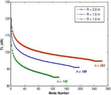
Figure 3 shows the convergence of TL curves at 10 kHz for a Glass/Epoxy cylindrical shell whose properties are listed in Table 1 (Daneshjou et al., 2009). As illustrated in Figure 3, by increasing the radius of the shell, the number of modes to achieve a converged solution is increased. As shown in Table 2, increasing the frequency has a direct effect on the convergence and hence more numbers of modes are needed at high frequency. In addition, as the accuracy of the results increase, the number of required modes also increases.
Material
Shell Cavity Ambient
Aluminum Steel Graphite/Epoxy Glass/Epoxy Boron/Epoxy Air Air
r (kg/m3)
2760 7750 1600 1900 1600 0.94 0.3795
11( )
E GPa 72 210 137.9 38.6 206 - -
22( )
E GPa 72 210 8.96 8.2 20.6 - -
12( )
G GPa 27.7 80.77 7.1 4.2 6.89 - -
13( )
G GPa 27.7 80.77 7.1 4.2 6.89 - -
23( )
G GPa 27.7 80.77 6.2 3.45 4.1 - -
u12 0.3 0.3 0.3 0.26 0.3 - -
/
( )
c m s - - - - - 328.5 296.6
) (
R m
1.5
) (
h mm 1.5
()
a
45Latin American Journal of Solids and Structures 11 (2014) 2039-2072
0 40 80 120 160 200 240 280
80 90 100 110 120 130
Mode Number
TL (
dB
)
R = 2.0 m R = 1.5 m R = 1.0 m
n = 140
n = 199
n = 264
Figure 3: Mode convergence diagram for Glass/Epoxy cylindrical shell at 10 kHz
Error Band (dB)
Radius (m)
Thickness (mm)
Frequency (Hz)
Mode
Number
6
10
-1 10
100 6
1000 20
10000 134
1.5 15
100 6
1000 28
10000 193
2 20
100 7
1000 32
10000 253
8
10
-1 10
100 6
1000 21
10000 140
1.5 15
100 7
1000 30
10000 199
2 20
100 8
1000 34
10000 264
Latin American Journal of Solids and Structures 11 (2014) 2039-2072 5 RESULTS AND DISCUSSION
In order to validate the present formulation and the developed code, the results obtained for the shells have been compared with those of the literature. Firstly, the analytical model presented by Lee and Kim (2003) and statistical energy analysis (SEA) are employed to validate the results for the special case of isotropic shell. Then, the model impedance method is utilized using the work presented by Koval (1979) for an orthotropic cylindrical shell.
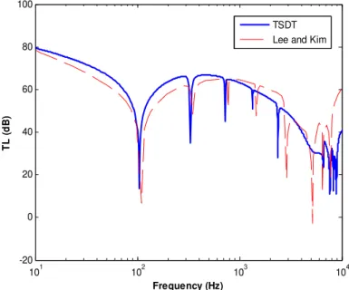
In Figure 4 the results of TSDT are compared with those of Lee and Kim's (2003) for an iso-tropic steel shell with characteristics as listed in Table 1. It can be seen that there is a good agreement between the results of two theories in the figure. The little differences are observed due to some numerical errors in calculation of the incident and transmitted powers in Kim's model.
101 102 103 104
-20 0 20 40 60 80 100
Frequency (Hz)
TL (
dB
)
TSDT Lee and Kim
Figure 4: Comparison of present study (TSDT) with Lee and Kim
Figure 5 compares the diffuse field transmission loss (TLave) obtained from the present model
with the numerical results achieved by statistical energy analysis approach using a wave number approach based on the proposed discrete laminate theory. Details of calculations of the required parameters (modal density, damping and coupling loss factor and radiation efficiency) for the SEA calculations are represented by Ghinet (2006) and Yuan (2012).
As illustrated in Figure 5, the predicted TLaveobtained from the present model reveals a good
agreement with the SEA simulation, particularly at high-frequency. SEA is based on simulating the vibro-acoustic energy flow between subsystems of the full system. It is very good in the study of sound and vibration transmission through complex structures at high frequencies. However, it is notreliable at low frequencies due to the statistical uncertainties that occur when there are few resonant modes in each of the subsystems. For this reason,a difference is observed at low
frequen-cies. If the isotropic shell is assumed to be steel shell, then fr = 432.9andfc = 3991.5. These
Latin American Journal of Solids and Structures 11 (2014) 2039-2072
102 103
0 10 20 30 40 50
Frequency (Hz)
TL
(
d
B
)
SEA
TSDT
f r = 432.9
f c = 3991.5
Figure 5: Comparison TLavefor random incident angles of present study (TSDT) with SEA
In Figure 6 the results of present study compared with those of Koval’s (1979) for a Graphi-te/Epoxy shell with the same condition as listed in Table 1. As it is demonstrated in the figure, some discrepancies are observed. It is happened as a result of using Flugge shell theory as well as applying only a transverse direction, in Koval’s study.
102 103 104
-20 0 20 40 60 80
Frequency (Hz)
TL (
d
B
)
TSDT Koval
Figure 6: Comparison of present study (TSDT) with Koval
Latin American Journal of Solids and Structures 11 (2014) 2039-2072
100 101 102 103 104
-20 0 20 40 60 80 100
Frequency (Hz)
TL
(
d
B
)
TSDT FSDT CST
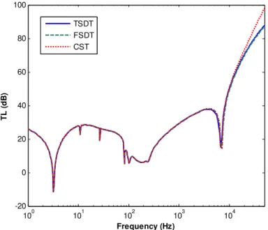
Figure 7: Comparison of present study (TSDT) with CST and FSDT for R/h=1000
100 101 102 103 104
-20 0 20 40 60 80 100 120 140 160 180
Frequency (Hz)
TL (
dB
)
TSDT FSDT CST
Latin American Journal of Solids and Structures 11 (2014) 2039-2072
100 101 102 103 104 0
50 100 150 200 250
Frequency (Hz)
TL
(
d
B
)
TSDT FDST CST
Figure 9: Comparison of present study (TSDT) with CST and FSDT for R/h=20
The results also indicate that TSDT are exactly similar with those of CST and FSDT in low fre-quencies. However, considerable errors are observed comparing the results of these theories at the high-frequency range, due to the effects of shear and rotation on TL. As depicted in Figures 8 and
9, with decrease of the ratio of R/h, the difference between TSDT and FSDT, is increased
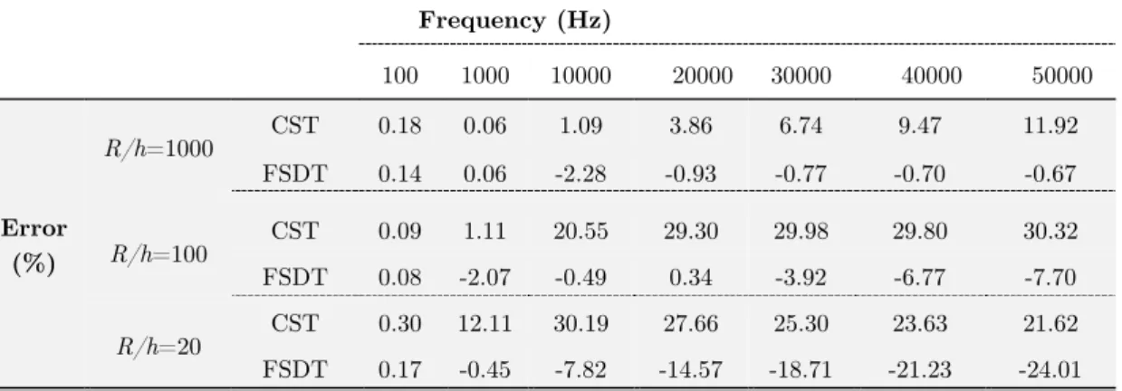
espe-cially at high frequencies. It appears that, the effects of shear deformation on sound transmission are increased when the wave lengths are short enough, i.e., of the same order or less than the thickness of the shell. Table 3 provides a comparison between the computed results from TSDT,
CST and FSDT with the different R/h ratios. The errors of these theories are presented in
Table 4 in comparison with TSDT. Overall, according to the results shown in Table 3, for thick shells, there are some discrepancies between TSDT and FSDT in high frequencies (about 24%
difference for R/h = 20) which is due to the less precise model of FSDT.
Frequency (Hz)
100 1000 10000 20000 30000 40000 50000
TL (dB)
R/h=1000
CST 6.47 29.21 50.53 73.14 84.37 92.14 98.12 FSDT 6.47 29.21 48.85 69.76 78.44 83.58 87.09 TSDT 6.46 29.19 49.99 70.42 79.05 84.17 87.67
R/h=100
CST 36.97 50.99 116.96 137.54 146.73 153.47 160.06 FSDT 36.97 49.38 96.55 106.74 108.46 110.23 113.36 TSDT 36.94 50.42 97.02 106.37 112.89 118.24 122.82
R/h=20
CST 53.46 98.17 159.67 177.05 186.47 193.05 196.89 FSDT 53.39 87.17 113.06 118.49 120.98 122.99 123.02 TSDT 53.30 87.56 122.65 138.69 148.81 156.15 161.89
Latin American Journal of Solids and Structures 11 (2014) 2039-2072
Frequency (Hz)
100 1000 10000 20000 30000 40000 50000
Error (%)
R/h=1000 CST 0.18 0.06 1.09 3.86 6.74 9.47 11.92 FSDT 0.14 0.06 -2.28 -0.93 -0.77 -0.70 -0.67
R/h=100 CST 0.09 1.11 20.55 29.30 29.98 29.80 30.32 FSDT 0.08 -2.07 -0.49 0.34 -3.92 -6.77 -7.70
R/h=20 CST 0.30 12.11 30.19 27.66 25.30 23.63 21.62 FSDT 0.17 -0.45 -7.82 -14.57 -18.71 -21.23 -24.01
Table 4: Error (%) in comparison to present study (TSDT) for different frequencies and R/h.
Figures 7 to 9 and Table 3 indicate that with increasing the thickness, TL is enhanced and coincidence frequency shifts backward. At high frequencies, the wave lengths are very short in comparison to radius of the shell. Therefore, the radius of the shell does not influence the TL. Moreover, the results for CST are more than those of FSDT and TSDT at high frequencies. It is due to the fact that the shear and rotation are both significant in sound power transmission in high frequency range whereas the CST is completely ignored them. Also, the results presented in
a forementioned figures and tables indicate that the difference between the results of TSDT and
FSDT will become more significant in high frequencies especially for thick shells. Therefore, the-need to use higher order shear deformation theory such as TSDT would increase. However, the FSDT seems to be a conservative criterion in comparison with TSDT in high frequencies as a result of demonstrating the least amounts of TL.
6 INVESTIGATIONS OF PARAMETERS
Figure 10 shows the effects of radius with R=0.5, 1.0 and 1.5 on TL. With increasing the shell
Latin American Journal of Solids and Structures 11 (2014) 2039-2072
100 101 102 103 104 -20
0 20 40 60 80
Frequency (Hz)
TL (
dB
)
R = 1.5 m R = 1.0 m R = 0.5 m
Figure 10: Investigation of R effect on TL curves
To investigate the effects of shell thickness, a comparison is made for three different shell
thi-cknesses of h = 1.5, 1.0 and 0.5 mm in Figure 11. As it is clear, with increasing the thickness, TL
is enhanced and coincidence frequency shifts backward.
100 101 102 103 104 -20
0 20 40 60 80
Frequency (Hz)
TL
(
dB
)
h = 1.5 mm h = 1.0 mm h = 0.5 mm
Figure 11: Investigation of h effect on TL curves
The results of present study for three different incident angles are shown in Figure 12. The
inspection of this figure represents that increasing of a, leads to impressive descend of TL in the