doi: 10.1590/0101-7438.2017.037.02.0403
MODEL AND SOLUTION METHOD TO A SIMULTANEOUS ROUTE DESIGN AND FREQUENCY SETTING PROBLEM FOR A BUS RAPID
TRANSIT SYSTEM IN COLOMBIA
Fabi´an Mart´ınez
1, Mar´ıa Gulnara Baldoqu´ın
2and Antonio Mauttone
3*Received April 4, 2017 / Accepted August 11, 2017
ABSTRACT.We propose a model and solution method to a simultaneous route design and frequency setting problem on a main corridor from one of the Bus Rapid Transit (BRT) Systems of Colombia. The proposed model considers objectives of users and operators in a combinatorial multi-objective optimization framework and takes into account real constraints on the operation of some Colombian BRT systems not found in previous models. The problem is solved heuristically by a Genetic Algorithm which is tailored from an existing work, to consider specific characteristics of the real scenario. The methodology is validated with current data from one of the most important bus corridors in a Colombian BRT system. The results obtained improve the current solutions for this corridor.
Keywords: public transportation, genetic algorithm, BRT.
1 INTRODUCTION
Public transport substantially determines the quality of life of the inhabitants of urban areas. A public transport system well designed and operated not only provides adequate mobility for users but also contributes to solving urban problems such as noise, traffic congestion, lack of public spaces, pollution, etc. Due to the high costs of implementing rapid transit systems based on rails, developing countries (especially in Latin America), as well as industrialized nations have been adopting Bus Rapid Transit (BRT) systems, which require less investment due to some factors as the use of more economical technologies (Hensher & Golob, 2008). Particularly in Colombia, 7 cities have BRT systems implementations, known as SITM (acronym in Spanish of Integrated System of Mass Transportation).
*Corresponding author.
1Departamento de Ingenier´ıa Civil e Industrial, Pontificia Universidad Javeriana, Cl. 18 #118-250, Cali, Valle del Cauca, Colombia. E-mail: [email protected]
2Departamento de Ciencias Matem´aticas, Escuela de Ciencias, Universidad EAFIT, Carrera 49 No. 7 Sur-50, Medell´ın, Antioquia, Colombia. E-mail: [email protected]
Bus Rapid Transit denotes a high-quality bus-based transit system that delivers fast, comfortable, and cost-effective services at metro-level capacities (Levinson et al., 2002). A BRT corridor is a section of road or contiguous roads served by one or multiple bus routes with a required minimum length of kilometers dedicated to bus lanes. There are some essential features that define a BRT as Dedicated Right-of-Way, Busway Alignment, Off-board Fare Collection and Platform-level Boarding.
All performance indicators of bus transport for monitoring and evaluating urban transport projects in Colombia (Ministerio de Transporte, 2008), reflect a main objective of improving mobility and quality of public transport services in strategic corridors of BRT systems. Although all Colombian cities have a similar regulatory framework, the design and implementation of BRT systems respond to the particularities of each city. According to data from one Survey of Quality of Life of the National Administrative Department of Statistics processed for the study developed in (Yepes et al., 2013), there has not been a strong impact of the BRT on the most vulnerable population. In (Yepes et al., 2013), as well as in the results of various surveys that take place annually, it is suggested that among the major challenges of urban transport systems in Colombia are the improvement of planning and operation of routes and the strengthening of the capacities of managers in optimizing routes.
In this work the problems of designing bus routes and their associated frequencies are studied simultaneously, in a corridor of one of the most representative BRT systems of Colombia, which we name SITM. The model and solution method proposed is based on the work of (Szeto & Wu, 2011); that work, although was not developed for BRT Systems, has some common features with the problem addressed in our study. Some works have been done for BRT systems in Colombia, in relation to the design of routes and frequencies, particularly for the BRT system in Bogot´a (Walteros et al., 2015). However, there are features and real assumptions for the SITM that have not been addressed in the literature, according to the extensive review made about models, methods and real applications to simultaneously solve the route design and frequency optimiza-tion problems.
The remainder of this paper is organized as follows. This section continues with the related work (Section 1.1) and our contribution (Section 1.2). In Section 2 the problem is formulated, high-lighting two subsections: how to determine the transfer stations when it is required by a route, based on the assignment model assumed (Section 2.3), and the solution method to determine the weighting factors in the weighted-sum approach considered for the multi-objective optimization model proposed (Section 2.4). In Section 3, the solution method is discussed, highlighting the differences with the method proposed in (Szeto & Wu, 2011). In Section 4, the proposed model and method are validated with real data of one of the main BRT corridors of the considered SITM. Finally, Section 5 concludes and gives some recommendations to continue this work.
1.1 Related work
TNDP (Transit Network Design Problem); in (Guihaire & Hao, 2008; Farahani et al., 2013; Oliveira & Barbieri, 2015) the authors use the terminology that we adopt to refer to this problem: TNDFSP (Transit Network Design and Frequencies Setting Problem). In (Farahani et al., 2013) is used the terminology Transit Network Design Problem (TNDP) exclusively to the design of routes of transit lines including the origins and destinations of the routes and the sequence of links visited.
Fern´andez, 1993; Wu & Florian, 1993; Wu et al., 1994; Cominetti & Correa, 2001; Cepeda et al., 2006). Some authors consider the capacity constraint of the buses as a constraint of the route optimization model, not in the assignment sub-model (Baaj & Mahmassani, 1991; Constantin & Florian, 1995; Leiva et al., 2010; Cancela et al., 2015). Baaj & Mahmassani (1991) intro-duced the term Load Factor, which is a qualifier that indicates, for each segment of a route, if the buses carry passengers standing. Spiess & Florian (1989) and Fern´andez (2013) proposed an assignment model on a transit network without congestion, which can be used as part of an op-timization model of routes and frequencies, controlling the decision variables in order to respect the load factor. In (Szeto & Jiang, 2014), the assignment formulation proposed by Spiess & Flo-rian (1989) is extended to capture transfer penalty. In our paper, the assignment model assumed is due to (Spiess & Florian, 1989), applied in the context of a simple corridor in a BRT system: a user knows reasonably different routes available for its trip; and he always selects, in his initial station, the first vehicle arriving of a feasible route, operating in the corridor. If the vehicle taken doesn’t arrive to the final station j, the passenger goes to the nearest station (k) of the station j that allows transfer with other(s) route(s) to arrive to the destination station j, and takes atkthe first vehicle which has a stop in j.
Two of the most common objectives considered in TNDFSP studies, reflecting the interest of the users and operators, are the total travel time (users) and the fleet size (operators). Total travel time (Lampkin & Saalmans, 1967; Dubois et al., 1979; Tom & Mohan, 2003; Bornd¨orfer et al., 2008; Cancela et al., 2015) is composed of: waiting time at station, in-vehicle travel time and transfer time. In-vehicle time is divided in two components: the time of vehicle in movement and the bus stop time in stations. The bus stop time in stations (also known as dwell time), in some real contexts as in our case study, is a constant that differs depending on the arrival station, and it is not considered in the reviewed papers. Few papers take into account other considerations as minimize excess travel time (Ceder & Wilson, 1986) and minimize excess time compared to the minimum path (Carrese & Gori, 2002). One way to model in a more realistic manner the interest of users is to consider minimizing the average deviation of the routes in proportion to the ideal travel time (travel time when there is no time for stops nor timeouts) and weighted by the number of users traveling. It is not the same, for example, the excess travel time, respect to the ideal, of 10 minutes in a trip of 50 minutes than in a trip of 20 minutes. This aspect, according to our review, has not been reflected in proposed models.
Transit Railway network is tested with various combinations of the weighting factors, where it is justified only some combinations where the values are zero or one. In (Cipriani et al., 2012) the objective function is defined as the weighted sum of operator’s costs, users’ costs and a penalty related to the level of unsatisfied demand. Such weights have been calibrated applying a sensitiv-ity analysis. In (Oliveira & Barbieri, 2015) the two objectives are to minimize both passengers’ costs (given by the total number of transfers, waiting and in-vehicle travel times) and operators’ costs (the total required fleet to operate the set of routes). The TNDFSP is addressed using a Genetic Algorithm (GA) and the bi-objective nature of the problem is solved using an alternat-ing objective function, which alternates from minimizalternat-ing users’ cost to minimizalternat-ing fleet at each generation of their GA. In some papers, the objective function is the sum of some other functions (Baaj & Mahmassani, 1991), either it is not specified how the weighting factors are obtained (Walteros et al., 2015) or weights are obtained in an experimental way, even if some applications of case studies are shown (Szeto & Wu, 2011). Another less referenced approach is multicriteria. In (Janarthanan & Schneider, 1986) the authors describe and apply a computer-based multicrite-ria method using concordance analysis to evaluate alternative transit system designs, including objectives, criteria, normalization methods and selection of weights in the weighted sum method. The normalization and the weighting, in the weighted sum approach, play an important role in ensuring the consistency of optimal (or near optimal) solutions obtained with the preferences expressed by the decision maker (DM) (Kaplinski & Tamoˇsaitien, 2015). In a real context, it is important to find a solution that is both Pareto (or near Pareto) optimal and also that satisfies to the DM. It is known that the weighted sum approach works well only when the Pareto front is convex. Even in this case, there are different approaches to achieve the weighting factors, some more effective than others. The weighting factors are generally composed by two factors, one being the weight given by the DM and the other, the normalization factor. The normalization is important not only when the objectives have different metrics, in order to obtain a unidimen-sional numerical form, but also when the range of solutions of the objectives are very different. There are different possible normalization schemas (Haftka & G¨urdal, 1992). Some of them have proved to be ineffective and are not practical (Grodzevich & Romanko, 2006). In our paper, the normalization and the weighting in the weighted sum approach are justified and contextu-alized to the case study presented, and according to our review about TNDFSP studies, this approach has not been used.
The resolution of TNDFSP has been tackled in the literature by means of different approaches, one of them metaheuristics. In that context, Genetic Algorithms (GA) has the most number of applications in TNDFSP (Pattnaik et al., 1998; Bielli et al., 2002; Ngamchai & Lovell, 2003; Tom & Mohan, 2003; Fan & Machemehl, 2004; Hu et al., 2005; Szeto & Wu, 2011). The proposed solution method in this paper is an adaptation of the GA proposed in (Szeto & Wu, 2011).
the reviewed papers make specific references to models and solution methods about TNDFSP, applied to BRT systems. The only case study found, applied to a simple corridor, is in (Larrain & Mu˜noz, 2008). However, although the real-world case study for the transport service of the city of Tin Shui Wai, Hong Kong, presented in (Szeto & Wu, 2011; Szeto & Jiang, 2014) is different from our real-world case, is the only paper of the reviewed literature that includes two common aspects with our problem: it considers a network with 28 stations connecting suburban areas to urban areas, size similar to the most corridors of the BRT studied in our paper, and the restriction of subsets of stations where the buses can start and return their trip.
Some of the reviewed papers are related to models and solution methods about TNDFSP applied to BRT systems, in particular on an isolated bus corridor (Larrain et al., 2010; Leiva et al., 2010; Scorcia, 2010; Chiraphadhanakul & Barnhart , 2013). In (Larrain et al, 2010), four parameters are defined for identifying corridor demand profiles, to determine what types of express ser-vices would be attractive on a bus corridor given the characteristics of its demand. The authors, using experimental simulations, conclude that a crucial parameter for determining the potential benefits of express services is the average trip length along the corridor and that the incorporation of express services is particularly attractive in corridors with demand profiles that increase or de-crease monotonically. In (Leiva et al., 2010), four optimization models are formulated, with and without vehicle capacity constraints and transfers between lines serving a corridor. These models can accommodate the operating characteristics of a bus corridor, given an origin–destination trip matrix and a set of services that are a priori attractive. A real-world case study of a bus corridor in the city of Santiago, Chile is presented. In (Chiraphadhanakul & Barnhart, 2013), the au-thors seek to modify a given bus schedule on a particular corridor by optimally reassigning some number of bus trips, to operate a limited-stop service in parallel with the local service, which serves every stop along the corridor. Scorcia (2010) proposes a methodology for the design and evaluation of service configurations for limited-stop services overlapping with local services. Although the TSW-HK case study presented in (Szeto & Wu, 2011) does not consider the simul-taneous definition of routes and frequencies for an isolated corridor in a BRT system, it has some aspects common to the BRT studied in this work, that are not identified in other papers reviewed. For example, it considers the definition of subsets of stations for the initial and final station of the routes and establishes a minimum frequency for each enabled route.
1.2 Contribution
The main contributions of this paper are:
1. The solution of a TNDFSP for a public transportation system with some characteristics not considered in the literature, according to the review done. We used a realistic scenario for which improved solutions were found by applying the proposed methodology.
2. The definition of components of the objective function, taking into account one aspect of the interest of the users, not previously contemplated.
3. The argumentation about the coefficients proposed in the weighted-sum approach, in the Multi-Objective Optimization Model considered.
4. Some modifications proposed to the model and solution method presented in (Szeto & Wu, 2011), in order to be able to apply such methodology to our case study.
2 PROPOSED FORMULATION
We propose a model to design simultaneously a set of routes for a corridor of a SITM and their associated frequencies with three objectives which reflect interest of users (two objectives) and operators (one objective).
The following hypotheses are considered:
• A simple BRT corridor of the SITM.
• The corridor is double lane. Each route has exactly the same stops in both directions between two points (origin and destination). There is a subset of stations for the start and return routes, because there are stations where the buses can not turn back towards the station from where it came.
• There are no restrictions about stations where the users can transfer.
• The total travel time considered is composed of: waiting time at station, in-vehicle time and transfer time. In-vehicle time is divided in two components: the time of vehicle in movement and the bus stop time in stations. The bus stop time in stations is a constant that differs depending on the arrival station.
• All users must have at least one route for travel from any station to another without transfer. • It is assumed the assignment model proposed by (Spiess & Florian, 1989).
Also, some specific restrictions are considered:
• A minimum frequency for the routes operating in a corridor for a specific time slot. • A maximum capacity of vehicles available and a maximum number of routes to be
consid-ered in a corridor.
• A maximum capacity of arrivals allowed at each station (number of vehicles/hour).
2.1 Notation and Modelling
Sets:
U set of nodes representing corridor stations,U ⊆N\{0}; Y set of nodes that allow south-south return (start),Y ⊆U;
V set of nodes that allow north-north return (final),V ⊆U,V∩Y = ∅; i,j,k,e indices for nodes;
n,m,q,r indices for routes,ǫ{1,2, . . . ,Rmax}.
Parameters:
ci j time in vehicle moving fromito j(hours); si average stop time ini(hours);
die number of passengers traveling from i toe (per unit time, at a given horizon);
fmin minimum frequency for routes operating in the corridor (number of vehicles/hour);
W available fleet size in the corridor;
Rmax maximum number of routes in the corridor;
C Ej maximum number of arrivals to j(number of vehicles/hour);
B1,B2,B3 weighting factors in the objective function for: total travel time of the users (B1), maximum deviation of travel (B2) and the number of vehicles assigned to routes (B3).
Decision variables:
Xi j n 1 if routenarrives nodej =iimmediately after nodei, and 0 otherwise, indicates the trajectory of the routenfromito jin both directions, if the routenis enabled; when it goes from north to southi < j and when it goes from south to north j<i;
X00n 1 if routenis disabled and 0 otherwise;
RTni j 1 if routenarrives to nodesiand j, consecutives or not in the routen; 0 otherwise;
Wi jn 1 if the routenhas a stop ini, no matter that does not stop in j, and has a stop in common betweeni and j with at least other route which has a stop at j station, 0 otherwise; j =i+1; j=i−1;
Oi jn 1 if the routenallows travel fromito j, either directly and/or with trans-fer, 0 otherwise;
fn frequency of routen, (vehicles/hour);
Tn cycle time of routen, in hours (time of the vehicle moving plus the time of each stop in all the trajectory of the routen, from north to south and south to north);
Vn number of vehicles needed to operate the route; Tie expected travel time fromitoe, (hours);
ti jn travel time fromi to j on the routen, beingi and j two stop points on the route, (hours);
Ti jn expected travel time fromito j usingnas initial route, wherei is a stop point of the routen, jmay or may not be a stopping point on the routen, (hours).
2.2 Mathematical programming formulation
min. z=B1 i∈U
e∈U
dieTie+B2
i
e(dieTie/cie)
i
edie
+B3 Rmax
n=1
Vn (1)
s.t
j∈Y∪{0}
X0j n=1, ∀n (2)
i∈V∪{0}
Xi0n=1, ∀n (3)
Xi j n−Xj in=0, ∀i, j ∈U, ∀n (4)
i∈Y∪{0},i<j
X0in≥Xj0n, ∀j ∈Y ∩V, ∀n (5)
j∈U j>i
Xi j n≤1, ∀i∈U∪ {0}, ∀n (6a)
i∈U i>j
Xi j n≤1, ∀j ∈U∪ {0}, ∀n (6b)
Tn= ⎡ ⎣
i∈U
j∈U,i=j
Xi j n(ci j+si) ⎤ ⎦
+
i∈U
(siXi0n+siX0in), ∀n (8)
Vn=Tnfn(1−X00n), ∀n (9)
Rmax
n=1
Vn≤W (10)
Rmax
n=1
i∈U∪{0}i<j
Xi j nfn(1−X00n)≤C Ej, ∀j∈U (11)
RTikn =Xikn+ j∈U k>j>i
Xi j nRTj kn, ∀i, k∈U, k>i, ∀n (12a)
RTikn =Xikn+ j∈U i>j>k
Xi j nRTj kn, ∀i, k∈U, k<i, ∀n (12b)
Rmax
n=1
RTi jn(1−X00n)≥1, ∀i, j ∈U, i= j (13)
tikn =Xikn(cik+si)
+
j∈U,i<j<k
Xi j nRTj kn(tnj k+ci j +si), ∀i, k∈U, k>i, ∀n (14a)
tikn =Xikn(cik+si)
+
j∈U,i>j>k
Xi j nRTj kn(t n
j k+ci j +si), ∀i, k∈U, k<i, ∀n (14b)
Wi jn =1−
∀m,m=n
k∈U,i<k<j
(1−RTiknRTk jm), ∀i, j ∈U, j >i, ∀n (15a)
Wi jn =1−
∀m,m=n
k∈U,i>k>j
(1−RTiknRTk jm), ∀i, j ∈U, j <i, ∀n (15b)
Oi jn =max{RTi jn, Wi jn}, ∀i, j ∈ U, j =i, ∀n (16)
Ti jn= ⎛ ⎜ ⎜ ⎜ ⎜ ⎜ ⎝ α Rmax m=1
fmOi jm(1−X00m) +ti jn
⎞ ⎟ ⎟ ⎟ ⎟ ⎟ ⎠
+ ⎛ ⎜ ⎜ ⎜ ⎜ ⎜ ⎜ ⎜ ⎜ ⎜ ⎜ ⎜ ⎜ ⎜ ⎜ ⎜ ⎜ ⎜ ⎜ ⎜ ⎜ ⎜ ⎜ ⎜ ⎜ ⎝ α Rmax m=1
fmOi jm(1−X00m) +tikn′
+ Rmax
m=1
⎛ ⎜ ⎜ ⎜ ⎜ ⎜ ⎜ ⎝
fmRTmk′j(1−X00m)
Rmax
q=1
fqRTqk′j(1−X00q)
⎞ ⎟ ⎟ ⎟ ⎟ ⎟ ⎟ ⎠ × ⎛ ⎜ ⎜ ⎜ ⎜ ⎜ ⎝ α Rmax q=1
fqRTqk′j(1−X00q)
+tkm′j
⎞ ⎟ ⎟ ⎟ ⎟ ⎟ ⎠ ⎞ ⎟ ⎟ ⎟ ⎟ ⎟ ⎟ ⎟ ⎟ ⎟ ⎟ ⎟ ⎟ ⎟ ⎟ ⎟ ⎟ ⎟ ⎟ ⎟ ⎟ ⎟ ⎟ ⎟ ⎟ ⎠
× Wi jn(1−RTni j)+M(1−Wni j)(1−RTni j) ∀i,j ∈U, j=i, ∀n (17)
Tie= Rmax
n=1
fnOien(1−X00n)
Rmax
m=1
fmOiem(1−X00m)
Tien, ∀i, e∈U, i =e (18)
In (1) three objectives with different weights are considered, to minimize:
• Total expected travel time (in hours), including stop times, initial wait time, the time of the vehicle in movement, and the waiting time for transfer;
• The average deviation of the routes in proportion to the ideal travel time and weighted by the number of users to carry;
• The number of vehicles required to operate routes.
The first objective aims for reducing the travel time of passengers with routes of greater demand, disfavoring users with low demand routes. The second objective is formulated considering that the same additional time for a couple of routes, where one of them takes much longer than another, is not equitable. The deviation should be measured in proportion to the ideal travel time (Tie/cie) rather than in units of time (Tie −cie). Additionally, it should be weighted by the number of passengers to maximize social benefit. The third objective aims to reduce the number of vehicles assigned to routes in order to improve the rate of passengers per kilometer, which will increase if the same demand is met with fewer vehicles. The units of each component of the objective function (1) are different: (number of passengers*hour), (dimensionless) and (number of vehicles) respectively; in Section 2.4 a method for normalization and weighting of these functions is proposed.
the same trajectory in both directions. Type restrictions (5) ensure that, for each enabled route, the initial station is before the return station. Type restrictions (6a) and (6b) ensure that each enabled route, on each direction, can stop at most once, in every possible station on the route. Type restrictions (7) ensure that the frequency of each of the routes enabled operating in the corridor is greater than the minimum frequency. Type restrictions (8) determine the cycle time of each route n, according to the appropriate parameters. Type restrictions (9) determine the number of vehicles required to operate each routen, if it is enabled, considering its cycle time and frequency. Type restrictions (10) ensure that the number of vehicles needed to operate the enabled routes does not exceed the number of vehicles available in the corridor.
Type restrictions (11) ensure that the number of arrivals at each station j does not exceed its capacity. It takes into account that the stations visited by each enabled route are the same in both directions. Restrictions (12a) and (12b) guarantee, by calculating the binary variablesRTnik,, for each routen, if it allows travel without transfer from any pointi to any pointkon the route. The two terms reflected in equations (12a) and (12b), the first with a binary variable, and the second with a sum expression, are exclusive and only one of them can take the value 1. When one of them takes the value 1 indicates that the routenallows to travel fromi tokwithout transfer. If the first term is 1, indicates that nodesi andk are consecutive stop stations on the route; if the second takes the value 1,iandkare not consecutive stop stations on the route.
Type restrictions (13) ensure that all users have at least one option for travel from any pointi to j without transfer. Type restrictions (14) calculate the travel time fromi tokon the routen, using equations (14a) and (14b) beingi andktwo stop points of the route. Type restrictions (15) determine, for each routen, the value of the binary variablesWi jn, if the route arrives toiand has a stop station in common betweeni and j with at least one other route that arrives to j. Type restrictions (16) determine, expressed in value taken by the binary variablesOi jn for each possible routen, and whatever the stations of the corridori, j, if it allows travel fromito jdirectly and/or performing transfer.
Type restrictions (17) estimate, expressed in the variables (Ti jn), the travel time fromi to j ifn is taken as initial route (Ti jn), whatever the stations (i,j) of the corridor are. The subscriptk′in (17) refers to a particular transfer station, determined by the strategy of trip exposed, beingtikn′
andtkm′jthe travel time on the routenfrom the stationi(respectively the travel time on the route mto the station j) wherek′is a transfer station. The procedure for calculating the value ofk′ is shown in Section 2.1. In the formulation ofTi jnin (17), the average waiting time for the arrival of the first vehicle, is given by:
⎛ ⎜ ⎜ ⎜ ⎜ ⎜ ⎝
α Rmax
m=1
Note that whenOi jm =1 andX00m=0 corresponds to α
a
fa
, α >0 (19)
wherea belongs to the subset of feasible routes (routes that allow travel from i to j directly and/or with transfer).
In (18) the expected travel timeTie is determined. The probability that a vehicle that operates on each of the routes that allow to travel directly or with transfer from the source station to the destination station, arrives at the station destination, is given by:
fnOien(1−X00n)
Rmax
m=1
fmOiem(1−X00q) = fn
a fa
, (for feasible routesa) (20)
The average waiting times and probabilities, given by equations (19) and (20) respectively, are defined based on the work done by (Spiess & Florian, 1989). In (Spiess & Florian, 1989; Fern´andez, 2013) different values that can takeα are indicated, according to the inter-arrival times of vehicles and the rate of arrival of passengers established for the transport system. In this paper, it is assumedα =1 supposing that the rate of arrival of passengers is uniform and that the distribution of time of inter-arrival of vehicles is exponential, with mean 1/
a fa, belonging ato the subset of feasible routes defined).
The model presented is not linear integer mixed,N P-hard, so it is proposed a Genetic Algorithm (GA) for its solution, a modification of the GA presented in the work of (Szeto & Wu, 2011), integrating in this algorithm a heuristic procedure for setting frequencies.
2.3 Determination of the transfer station
As stated in Section 1.1, the assignment sub-model greatly influences the particular optimiza-tion model of routes and frequencies. In the proposed formulaoptimiza-tion, the transfer staoptimiza-tion selected by users impacts the total travel time for a given solution. In real life, each user chooses the transfer station according to a particular criterion. When a user has several options, he could choose the nearest transfer station, the last transfer station, or any transfer station between both. To avoid different total travel time for a same set of routes with a same frequency setting, we assume that users always choose the closest station to the destination station. It must be clear that unless the determination of the transfer station is random, any criteria used to determine the transfer station is equally valid, depending on the real scenario where it is applied.
Algorithm 1
Letnbe the initial route andmthe enabled route(s):
For a route that allows travel only with transfer fromito j:EC= ∅
V Kis a vector of zeros of length equal toRmax−nR=max1 X00; Ifi< j:
k′=i;
For each enabled route m except the routen
If the routemarrives to the station j, and has at least one stop station in common with the routenbetweeniandj:
Identify arrival stations in common betweeniandjwith the route
nand add them to the setEC; End
k′=max{EC};
Addk′to the vectorV K in the positionm; End
k′=max(V K); End;
Ifj<i:
k′=i;
For each enabled routemexcept the routen
If the routemarrives to the station j, and has at least one stop station in common with the routenbetween jandi:
Identify arrival stations in common betweenjandiwith the route
nand add them to the setEC; End
k′=min{EC};
Addk′to the vectorV K in the positionm; End
k′=min(V K); End;
Identify the route(s) of transfer ink′by the position ofk′>0 in theV K vector. End.
2.4 Normalization and weightings in the objective function
The normalization approach used is a variation of the method described in (Grodzevich & Ro-manko, 2006) using the ideal or utopian solution (zideal) and Nadir (znadir). Given the above values, a function f(x)is represented on a scale between zero and one, using the function
f1(x)= f(x)−z nadir
zideal−znadir
zidealis obtained by taking the objective value offered by the current solution (sa) reduced by a percentageδ. The objective function (1) is transformed into (21):
maxz = B1 i∈U,e∈UdieTie
−sa1
−δsa1
+ B2
⎡ ⎢ ⎣
i∈U,e∈U(dieTie/cie)
i∈U,e∈Udie −sa2
−δsa2
⎤ ⎥ ⎦
+B3
Rmax
n=1 Vn−sa3 −δsa3
(21)
where:
B1+B2+B3=1; B1,B2,B3≥0; δ >0;
sa1: the value of
i∈U,e∈UdieTiegiven by the current solution; sa2: the value of
i∈U,e∈U(dieTie/cie)
i∈U,e∈Udie given by the current solution;
sa3: the value ofRmax
n=1 Vngiven by the current solution.
The valuesB1,B2andB3(weighting factors in the objective function) are not determined exper-imentally. It is used the Analytic Hierarchy Process (AHP) (Saaty, 1994). In Section 4 the values determined by the company are indicated, using the AHP methodology.
3 SOLUTION METHOD
We adopt the two crossing operators proposed by (Szeto & Wu, 2011) and two of the four mu-tation operators. We use the same diversity control mechanism for the selection of individuals of each new generation. We do not use a stop sequence improvement procedure, since over a trunk corridor of SITM, the routes are defined as totally ordered sets, since for any set of stops there exists only one sequence. Note that for similar instances in terms of number of stations and size of origin-destination matrix, the search space in TSW-HK is much larger than the one corresponding to the SITM, even though the formulation of (Szeto & Wu, 2011) is limited on the maximum number of intermediate stops for each route.
(a) The TSW-HK bus network. (b) A single corridor in the BRT system.
Figure 1– The investigated networks in the two study cases.
of individuals is constant. The process is repeated until a pre-specified number of generations is attained.
Figure 2– Structure of the proposed Genetic Algorithm.
3.1 Solution representation and generation of the initial population
A chromosome (individual) of the GA represents a set of Rmax routes. In the SITM, a route rn is a totally ordered set of stationsi ∈ U. The chromosome is a matrix of Rmaxrows and number of columns equal to the number of stations of the corridor. A random feasible individual which fulfills type restrictions (2)-(6) and (13) is generated by using the procedure depicted in Algorithm 2. The process is repeated a number of times necessary to complete the size of the population. In the initialization procedure, first, the start and returning station of each of the Rmaxroutes are assigned. It is guaranteed that at least one route has the first station as the starting one and the last station as the returning one. Then, combinations (i,j) are inserted randomly among theRmaxroutes, in order to fulfill the type restriction (13). After sorting the stations on each route and eliminating repeated stations, the types of restrictions (2)-(6) are fulfilled.
3.2 Heuristic procedure for frequency setting
Algorithm 2
For routen=1 Initial node=1;
Returning node=last station from setU; End;
For routen=2. . .Rmax
Select randomly an initial nodei∈Y and a returning node j>i∈V for routen; Next route;
End; Fori∈U
Forj>i∈U
Ifiandjare not present at any route of the individual:
Select randomly a route from the set of routes having initial station beforeiand returning station after j; insert stationiandj; End;
Next j; End; Nexti; End;
For routen=1. . .Rmax
Sort routenand delete repeated stations; Next route;
End.
where the first one represents the number of unused vehicles. The second position corresponds to the number of vehicles assigned tor1and so on. Taking into account that fn = Vn/Tn (9), the following procedure is used to generate (if possible) a feasible solution with respect to type restrictions (7), (10), (11) and (13), wheremandnare positions in the solution vector. In order to calculate the number of vehicles necessary to operate each route with minimum frequency fmin, we create a vector withRmaxpositions with these values, denoted asV N.
According to the procedure depicted in Algorithm 3, the type restriction (10) always is fulfilled since the sum of all values in the solution vector is equal toW. However, in order to fulfill type restrictions (7), (11) and (13), for each violated restriction we include a penalization in the fitness evaluation and the selection of survival individuals discards unfeasible elements. As a result of this procedure we can obtain disabled routes, i.e., routes without vehicles to operate.
Algorithm 3
LetS = (R,F), where R is the set of routes, F the set of frequencies forR, andF[q]the element in the positionqfrom vectorF.
LetV N a vector withRmax positions, whereV N[q]is the element in the positionqof the vector.
LetV Sa vector with Rmax+1 positions, whereV S[k]is the element in the positionkof the vector; values inV Sfrom position 2 are those of vectorV N.
Letnvnbe the sum of all values inV N.
q=1
Whileq≤Rmax
V N[q] =mi n{k∈N|k≥ f minTq}
F[q] =V N[q]/T q q=q+1
End.
Ifnvn is less than the number of available vehiclesW, then V S[1] is equal to W −nvn, otherwise is zero.
vae=nvn−W; Whilevae>0:
Select randomly a numberkfrom the set{k∈N|2≤k≤Rmax+1};
V S[k] =V S[k] −1;
vae=vae−1; End.
EvaluateSusing (21); Form=1
V P= {m+1. . .Rmax+1}; WhileV P= ∅:
Select randomly an elementnfrom setV P;
V P=V P− {n};
While the value of the objective function (1a) is improved or unchanged and the numberV S[m]is greater than zero:
V S[m] =V S[m] −1; V S[n] =V S[n] +1; F[n−1] =V S[n]/Tn−1; evaluateSusing (21)
End;
While the value of the objective function (1a) is improved or unchanged and the numberV S[n]is greater than zero:
V S[n] =V S[n] −1; V S[m] =V S[m] +1; F[n−1] =V S[n]/Tn−1; evaluateSusing (21);
End; End; End
Algorithm 3 – (continuation)
Form=2. . .Rmax:
V P= {m+1. . .Rmax+1}; WhileV P = ∅:
Select randomly an elementnfrom setV P;
V P=V P− {n};
While the value of the objective function (1a) is improved or unchanged, the numberV S[m]is greater than zero and routes(m−1)
and(n−1)are different:
V S[m] =V S[m] −1; V S[n] =V S[n] +1; F[n−1] =V S[n]/Tn−1;
F[m−1] =V S[m]/Tm−1; evaluateSusing (21) End;
While the value of the objective function (21) is improved or unchanged, the numberV S[n]is greater than zero and routes(m−1)
and(n−1)are different:
V S[n] =V S[n] −1; V S[m] =V S[m] +1; F[n−1] =V S[n]/Tn−1;
F[m−1] =V S[m]/Tm−1; evaluateSusing (21) End;
End; Nextm; End
For each pair of identical routes, take the number of vehicles assigned to both and assign them only to one route;
End.
3.3 Crossover and mutation operators
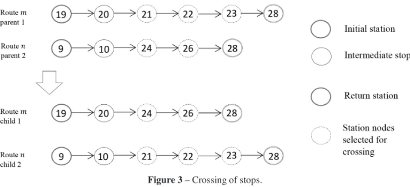
As in (Szeto & Wu, 2011), we propose two crossing operators: one for crossing routes and other for crossing stops between routes. Both operators are applied to individuals selected from the population by using the roulette method. For each crossing, one operator is selected randomly. The operator for crossing routes exchanges sets of routes between two individuals, as it is done in (Szeto & Wu, 2011). We generate two numberskandl,{k,l ∈N|1=k,l =Rmax,k=l}, then, the routes betweenrkandrl are exchanged between the selected individuals.
routen from parent 2 (having the same return station) are selected randomly. Then, two nodes between the initial and returning stations of the shortest route (routemfrom parent 1) are selected randomly (nodes 21 and 27 in the example). At last, the nodes between the selected ones are exchanged to generate routemin child 1 and routenin child 2.
Figure 3– Crossing of stops.
There are two situations in which the operator for crossing stops cannot be applied. First, when the second parent does not have a route with the same returning point as the one of the route selected from the first parent. Second, when some of the selected routes has consecutive initial and returning stations, since there are not nodes to exchange. If some of these situations arise, the process is repeated. If after a given number of trials, a pair of routes to apply the operator for crossing stops is not found, the crossing of routes is applied. The operator for crossing stops proposed by (Szeto & Wu, 2011) selects randomly sequences of intermediate stops from each route, and the stops are exchanged. This idea cannot be used in our method, since it would generate unfeasible solutions with respect to the type restriction (2).
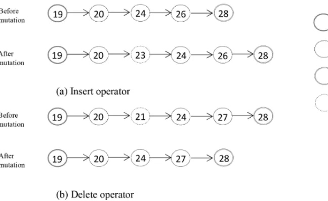
In (Szeto & Wu, 2011), four mutation operators are proposed: (a) insert, (b) delete, (c) swap and (d) transfer. In this work, we use only the insert and delete operators (Fig. 4) since the application of the other two operators would generate solutions which violate the type restrictions (2) and (3). The used operators generate a perturbation in a single route selected randomly from the individual. The insert (delete) operator inserts (deletes) a node to (from) the selected route. In both operators, the node to be inserted or deleted is selected randomly from the positions between the initial and returning routes; it could not belong to the route. The route remains unchanged if the node to delete does not belong to the route or if the node to insert already belongs to the route. A route with consecutive initial and returning stations cannot be mutated. For each mutation, the specific operator is determined randomly. The mutation probability is a parameter of the algorithm.
3.4 Repair operator
The repair operator works as follows. For each individual which violates the type restriction (13), each missing combination of stops (i,j) is inserted in routes selected randomly from the set of routes having initial station before nodei and returning station after node j. Then, repeated nodes from each route of repaired individuals are eliminated.
Figure 4– Mutation operators.
3.5 Control of diversity
In order to control the diversity of the population, we implement the mechanism of survival probability assignment proposed in (Szeto & Wu, 2011), which is based on the DCGA (Diversity Control Genetic Algorithm) proposed in (Shimodaira, 2001). It works by sorting decreasingly the individuals of the population with respect to their fitness values and selecting randomly according to probability P(s) (see expression 22), which is based in the Hamming distance with respect to the individual with highest fitness in the population. The Hamming distance between two sequences of characters with same length is the number of differences between each position of the sequence (it measures the minimum number of substitutions required to change from one sequence to the other). This method favors individuals with good fitness values and high contribution to diversity.
P(s)=
(1−c)h L +c
a
(22)
The Hamming distance was defined originally for binary codes. For that reason, its computation for solutions of our problem is not immediate. For that reason, Szeto & Wu (2011) propose defining the Hamming distance as the number of different pairs of consecutive nodes between two routes, each one from a different individual. The DCGA proposed by Shimodaira (2001) is applied in this work by applying the procedure depicted in Algorithm 4.
Algorithm 4
Delete repeated and/or not feasible individuals inM;
Select the best individualIbestfromMto be part of the following generation:
N G= {Ibest}. M′= M\{Ibest};
t p: size of population;
While there are individuals inM′and the number of individuals in N Gis not greater thant p:
e=random number in[0,1];
Is =best individual ofM′; Ife< P(Is):
includeIsin the new generationN G; End
M′=M′\{Is}; End
While the number of individuals inN Gis not greater thant p:
Create randomly an individual following the initialization procedure.
If after setting its frequencies it fulfills the type of restrictions (7), (11) and (13), it is included inN G;
End.
By selecting solutions according to the Hamming distance with respect to the best solution (and not considering survival individuals identical in each generation), we reduce the risk of losing information generated by moderately good individuals, which could be used afterwards to find the global optimum. The loss of good solutions depends on the selective pressure induced by the setting of values to parametersa andc. A reduction in the selective pressure induced by this mechanism of diversity control, affects negatively the efficiency of the GA. However, the definition of routes in the corridor of SITM is a strategic decision which does not require a quick response.
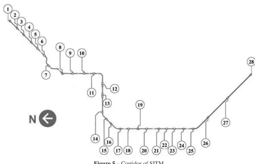
4 VALIDATION OF THE PROPOSED METHOD
Data was provided by the transit operator of the corridor, including current frequencies and maximum number of routes. The corridor comprises 28 stations (Fig. 5), where:
Other data considered in the case study comprises:
• Capacity of the stations, expressed in number of vehicles per hour.
• Origin-Destination (OD) matrix, expressed in passengers per hour. The number of passen-gers traveling between each pair of stations over a corridor depends on the time of day (peak, off-peak), the type of day (Monday-Friday, weekends) and the season of the year. The OD matrix provided by the operator corresponds to the time period between 6:00 and 7:00 in the morning of a representative working day. These data correspond to the period of highest demand in the system (Ministerio de Transporte, 2008). The EMME software (INRO, 2017) for transit planning was used by the operator to obtain an OD matrix update, by applying a growth factor method based on a historical OD matrix. • Average stopping (dwell) time at each station (in seconds).
• Travel time of vehicles (in hours) between each pair of consecutive stations of the corridor, in the same time horizon as the OD matrix. That time can be obtained by two different ways. First, in terms of the average speed and the distance between stations, ignoring such factors like traffic flow and lights, real-time control procedures and driver behavior, among others. The second way is based on the average of observed (historical) travel time in the time horizon; this considers all the factors influencing the parameter of interest. From the point of view of our optimization model, the travel time between two consecutive stations is constant (the same for every different solution to the problem). Therefore, the travel time is relevant only for computing frequencies, since the reduction in the expected travel time and the average deviation of the routes depend on the number of stops, the stopping time at each station, the number of transfers and the waiting time. For this reason, measures which consider minimization of number of stops and/or number of transfers, maximizing the number of direct trips or setting limited-stop routes, are good objective functions when we aim to maximize the level of service subject to a level of profit of the operators. We used a computer with Core i7 processor and 4 GB of RAM. Table 1 shows results of apply-ing the AHP methodology in order to weight the objectives. The consistency ratio (CR) value indicates the validity of the comparisons between each objective made by the Decision Maker (DM). In this instance, the objective function (1) only allows solutions that adapt to the specific needs of the DM by this weighting of the objectives.
Currently there are three routes operating in the corridor. The first one stops at every station. The second one traverses the whole corridor and stops only at one station. The last one covers only a portion of the corridor. The attributes of each route are given in Table 2. We set as minimum allowable frequency, the value corresponding to the current route with minimum frequency, that is fmin =8.33 vehicles per hour (Route 2).
Figure 5– Corridor of SITM.
Table 1 – Weighting of the objectives. A (total expected travel time), B (average deviation of the routes in proportion to the ideal travel time), C (number of vehicles required to operate the routes).
A B C Ratio Scale of Priority
A 1 5 6 B1=0.71
B 1/5 1 3 B2=0.2
C 1/6 1/3 1 B3=0.09
1.37 6.33 10 Consistency Ratio (CR)=0.08
Table 2– Current routes and frequencies.
Route Number of Frequency Stations
vehicles assigned (vehicles/hour)
1 22 9.47 1,2,3,4,5,6,7,8,9,10,11,12,13,14,15,16,
17,18,19,20,21,22,23,24,25,26,27,28
2 18 8.33 1,2,3,4,8,12,16,17,19,21,24,25,26,28
The number of routes enabled in a given individual depends on the number of available vehicles, the capacity of the stations and the minimum allowed frequency. In order to state the maximum number of routesRmaxover the corridor, we propose the following formulation:
Rmax=min{max{k∈N|k=C Emin/fmin},min{k∈N|k=W/nvmax}},
whereC Emin is the capacity of the station with minimum capacity andnvmaxis the number of vehicles necessary to operate the longest route (it passes by all stations and stops at all of them) with minimum frequency. The term max{k∈N|k=C Emin/fmin}considers the fact that a feasible solution should allow the maximum number of routes and all of them can arrive to the station(s) with lowest capacity. In our case max{k∈N|k=42/8.33} =5. The term min{k∈ N|k = W/nvmax}considers the fact that the available fleet should be sufficient to enable the maximum number of routes, thus ensuring the fulfillment of minimum frequency, assuming that not all routes will usenvmaxvehicles. In our casenvmax =20, min{k ∈ N|k =52/20} =3, thereforeRmax=3.
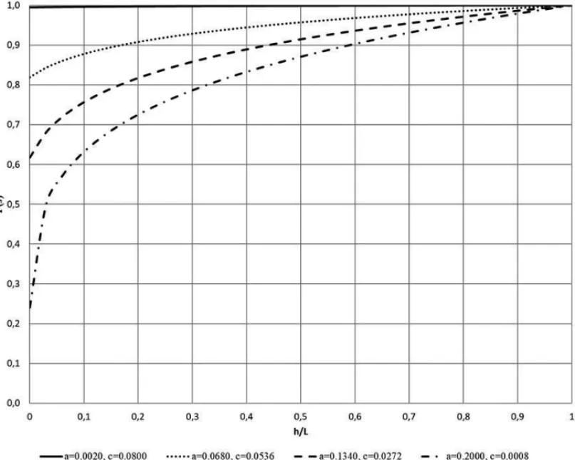
We set the constantδ(normalization of the objective function) as 0.05. The size of the population is 10. We generate the same number of children in the crossover operator and all of them are mutated, where each operator (insert and delete) has the same probability (0.5) of being applied. For setting these parameters, we took the work of (Szeto & Wu, 2011) as reference. Then, we tuned the parametersaandc. Figure 6 shows different combinations of them. The higher is the area below the curve (P(s)vs.h/L), the higher is the selective pressure. Forc=1 the selection of survivals is totally elitist (only the best individuals survive). Forc=0 anda=1, the probability of selection is directly proportional toh/L. Assuming thataandcare real numbers in the range [0,1]with at least four significant numbers, we could generate more than 99 million of different combinations.
In order to adjust parametersaandc, we tested different combinations having a value forP(s)less than 0.01 whenh=0, considering that if we allow surviving the best individual, the probability of selectionP(s)should be small. Among the combinations tested, the one which exhibited best performance corresponds toa =0.9999 andc =0.0001. Figure 7 illustrates the convergence process of the GA; we can note that convergence is attained after 300 generations. This execution takes approximately 180 minutes.
To adjust the population size (t p) we varied its value between 10 and 20 individuals. For those ex-treme values, the solutions obtained do not exhibit significant differences. However, fort p=20 the number of generations needed to attain convergence increases, therefore, also the execution time increases. For that reason, we set the valuet p=10.
4.1 Results
Table 3 shows results obtained by running the GA with the parameters adjusted as explained above. Table 4 shows the best configuration of routes and frequencies obtained.
Figure 6– Surviving probability of an individual for different combinations ofaandc.
Table 3– Solution obtained with the proposed method.
Average last Best Current generation individual solution
Objective function (21) 0.9547 0.9597 0.0000
Expected total travel time (thousand of hours) 6.7620 6.7610 7.0252
Average deviation of routes 1.50 1.49 1.67
Required number of vehicles 52 52 52
Figure 7– Convergence of the proposed Genetic Algorithm.
Table 4– Best configuration of routes and frequencies obtained by the proposed method.
Route Number of Frequency Stations
vehicles assigned (vehicles/hour)
1 30 12.9199 1,2,3,4,5,6,7,8,9,10,11,12,13,14, 15,16,
17,18,19,20,21,22,23,24,25,26,27,28
2 22 9.6305 1,2,3,4,8,9,10,11,12,13,14,15,16,17,18,
19,21,22,23,24,25,26,27,28
5 CONCLUSIONS AND FUTURE WORK
For future work, we identify three main lines which deserve attention. First, a study of the passen-ger behavior observed in the scenario where the methodology is applied would allow for tailoring the assignment sub-model adopted. Moreover, that sub-model could include different types of behavior, for example considering stochastic perception of passenger travel time. Second, assign more penalization to the perception of dwell time (the time buses stop at the stations) would en-rich the passenger behavior model. Users that perform short trips will be indifferent to that time, whereas passenger performing long trips will be sensitive and therefore, they will prefer express services (Larra´ın, 2013). Third, taking into account that in this study the proposed methodology is applied only to a trunk corridor, the joint optimization of both trunk and feeder routes would be more realistic, since relevant interplays are observed between these different types of routes. Note that a portion of the total demand for public transportation, is generated (either produced or attracted) at zones reachable only by feeder routes. Finally, applying the proposed method-ology to other SITM scenarios would enrich the study, contributing to the generalization of the proposal.
REFERENCES
[1] BAAJMH & MAHMASSANIHS. 1991. An AI-based approach for transit route system planning and desing.Journal of Advanced Transportation,25(2): 187–210.
[2] BIELLIM, CARAMIAM & CAROTENUTOP. 2002. Genetic algorithms in bus network optimization.
Transportation Research Part C: Emerging Technologies,10(1): 19–34.
[3] BORNDORFER¨ R, GROTSCHEL¨ M & PFETSCHM. 2007. A column-generation approach to line planning in public transport.Transportation Science,41(1): 123–132.
[4] BORNDORFER¨ R, GROTSCHEL¨ M & PFETSCHM. 2008. Models for line planning in public trans-port. In:Computer-Aided Systems in Public Transport[edited by M. HICKMAN, P. MIRCHANDANI & S. VOSS] Springer Berlin/Heidelberg, 363–378.
[5] CANCELAH, MAUTTONEA & URQUHARTME. 2015. Mathematical programming formulations for transit network design.Transportation Research Part B: Methodological,77: 17–37.
[6] CARRESES & GORIS. 2002. An urban bus network design procedure.Applied Optimization,64: 177–196.
[7] DECEAJ & FERNANDEZ´ E. 1993. Transit assignment for congested public transport systems: An equilibrium model.Transportation Science,27(2): 133–147.
[8] CEDERA & WILSONNHM. 1986. Bus network design.Transportation Research Part B: Method-ological,20(4): 331–344.
[9] CEPEDA M, COMINETTI R & FLORIAN M. 2006. A Frequency-Based Assignment Model for Congested Transit Networks with Strict Capacity Constraints: Characterization and Computation of Equilibria.Transportation Research Part B: Methodological,40(6): 437–459.
[10] CHIRAPHADHANAKUL V & BARNHART C. 2013. Incremental bus service design: combining limited-stop and local bus services.Public Transport,5: 53–78.
[12] COMINETTIR & CORREAJ. 2001. Common-lines and passenger assignment in congested transit networks.Transportation Science,35(3): 250–267.
[13] CONSTANTINI & FLORIANM. 1995. Optimizing frequencies in a transit network: a nonlinear bi-level programming approach.International Transactions in Operational Research,2(2): 149–164.
[14] DUBOISD, BELG & LLIBREM. 1979. A set of methods in transportation network synthesis and analysis.The Journal of the Operational Research Society,30(9): 797–808.
[15] FAN W & MACHEMEHLRB. 2004. Optimal transit route network design problem: Algorithms, implementations, and numerical results. Technical Report No. SWUTC/04/167244-1. Austin, Texas: Center for Transportation Research, University of Texas.
[16] FARAHANIRZ, MIANDOABCHIE, SZETOWY & RASHIDIH. 2013. A review of urban transporta-tion network design problems.European Journal of Operational Research,229(2): 281–302.
[17] FERNANDEZ´ A. 2013. Modelos matem´aticos de asignaci´on de tr´ansito, aplicaci´on a la red metropo-litana de la ciudad de M´exico y sus efectos en el STC-Metro. Tesis de Maestr´ıa en Ciencias, Depar-tamento de Matem´aticas Aplicadas e Industriales, Universidad Aut´onoma Metropolitana-Iztapalapa.
[18] GRODZEVICHO & ROMANKOO. 2006. Normalization and Other Topics in Multi-Objective Opti-mization. Proceedings to theFields-MITACS Industrial Problem Solving Workshop, Toronto, Canada.
[19] GUANJ, YANGH & WIRASINGHES. 2006. Simultaneous optimization of transit line configuration and passenger line assignment.Transportation Research Part B: Methodological,40(10): 885–902.
[20] GUIHAIRE V & HAO J-K. 2008. Transit Network Design and Scheduling: a Global Review.
Transportation Research Part A: Policy and Practice,42: 1251–1273.
[21] HAFTKART & G ¨URDALZ. 1992. Elements of Structural Optimization. Springer Netherlands.
[22] HENSHERDA & GOLOBTF. 2008. Bus rapid transit systems: a comparative assessment. Trans-portation,35(4): 501–518.
[23] HU J, SHI X, SONGJ & XUY. 2005. Optimal design for urban mass transit network based on evolutionary algorithms. In: Advances in natural computation [edited by L. WANG, K. CHEN& Y. ONG], Springer Berlin/Heidelberg, 429–429.
[24] INRO. 2017. INRO Software. Available at:http://www.inrosoftware.com. Last accessed March 1st, 2017.
[25] JANARTHANANN & SCHNEIDERJ. 1986. Multicriteria evaluation of alternative transit system designs.Transportation Research Record,1064: 26–34.
[26] KAPLINSKIO & TAMOˇSAITIENJ. 2015. Analysis of normalization methods influencing results: a review to honour Professor Friedel Peldschus on the occasion of his 75th birthday.Procedia Engi-neering,122: 2–10.
[27] LAMPKINW & SAALMANSPD. 1967. The design of routes, service frequencies, and schedules for a municipal bus undertaking: A case study.Operational Research Quarterly,18(4): 375–397.
[28] LARRA´INH. 2013. Dise ˜no de Servicios Expresos para Buses. PhD Thesis. Pontificia Universidad Cat´olica de Chile.
[30] LARRAINH, GIESENR & MUNOZ˜ J. 2010. Choosing the right express services for bus corridor with capacity restrictions.Transportation Research Record,2197: 63–70.
[31] LEIVA C, MUNOZ˜ J, GIESENR & LARRA´INH. 2010. Design of limited-stop services for an ur-ban bus corridor with capacity constraints.Transportation Research Part B: Methodological,44(10): 1186–1201.
[32] LEVINSONHS, ZIMMERMANS, CLINGER J & RUTHERFORDCS. 2002. Bus rapid transit: An overview.Journal of Public Transportation,5(2): 1–30.
[33] MINISTERIO DE TRANSPORTE. 2008. Seguimiento y Evaluaci´on del Transporte Urbano, In-dicadores. Colombia. Available at: http://portal.mintransporte.gov.co:8080/ transporte_urbano/indicadores.asp. Last accessed March 1st, 2017.
[34] NGAMCHAIS & LOVELLDJ. 2003. Optimal time transfer in bus transit route network design using a genetic algorithm.Journal of Transportation Engineering,129(5): 510–521.
[35] NGUYENS & PALLOTTINOS. 1988. Equilibrium Traffic Assignment for Large Scale Transit Net-works.European Journal of Operational Research,37: 176–186.
[36] OLIVEIRAR & BARBIERIC. 2015. Efficient transit network design and frequencies setting multi-objective optimization by alternating multi-objective genetic algorithm.Transportation Research Part B: Methodological,81(2): 355–376.
[37] PATTNAIKSB, MOHANS & TOMVM. 1998. Urban bus transit route network design using genetic algorithm.Journal of Transportation Engineering,124(4): 368–375.
[38] SAATY T. 2008. Decision making with the analytic hierarchy process.International Journal of Services Sciences,1(1): 83–98.
[39] SCORCIAH. 2010. Design and evaluation of BRT and limited-stop services. Master Thesis. Mas-sachusetts Institute of Technology.
[40] SHIMODAIRAH. 2001. A diversity-control-oriented genetic algorithm (DCGA): Performance in function optimization. Proceedings of the 2001 Congress on Evolutionary Computation, Seoul, Korea.
[41] SPIESSH & FLORIANM. 1989. Optimal strategies: A new assignment model for transit networks.
Transportation Research Part B: Methodological,23(2): 83–102.
[42] SZETOWY & JIANGY. 2014. Transit route and frequency design: Bi-level modeling and hybrid artificial bee colony algorithm approach.Transportation Research Part B: Methodological,67: 235– 263.
[43] SZETOWY & WUY. 2011. A simultaneous bus route design and frequency setting problem for Tin Shui Wai, Hong Kong.European Journal of Operational Research,209(2): 141–155.
[44] TOMVM & MOHANS. 2003. Transit route network design using frequency coded genetic algorithm.
Journal of Transportation Engineering,129(2): 186–195.
[45] WALTEROS JL, MEDAGLIAAL & RIANO˜ G. 2015. Hybrid Algorithm for Route Design on Bus Rapid Transit Systems.Transportation Science,49(1): 66–84.
[47] WUJH, FLORIANM & MARCOTTEP. 1994. Transit Equilibrium Assignment: A Model and Solu-tion Algorithms.Transportation Science,28(3): 193–203.
[48] YEPES T, JUNCA JC & AGUILAR J. 2013. La integraci´on de los sistemas de transporte urbano en Colombia, una reforma en transici´on. FEDESARROLLO, Centro de Investigaci´on Econ´omica y Social. Available at: http://www. fedesarrollo.org.co/wp-content/uploads/2011/08/La-integraci%C3% B3n-de-los-sistemas-de-transporte-urbano-en-Colombia-Findeter.pdf. Last accessed March 1st, 2017.
[49] ZHAOF & ZENGX. 2007. Optimization of user and operator cost for large scale transit networks.