J. Braz. Soc. Mech. Sci. & Eng. vol.32 número1

Marcelo M. Ganzarolli

[email protected]

Carlos A. C. Altemani

[email protected] State University of Campinas – UNICAMP Faculty of Mechanical Engineering Department of Energy 13083-860 Campinas, SP, Brazil

Nitrogen Charge Temperature

Prediction in a Gas Lift Valve

The operation of a class of retrievable gas-lift valves (GLV) is controlled by the axial movement of a bellows. One force acting on the bellows is due to the pressure exerted by the nitrogen gas contained in the GLV dome. It depends on the nitrogen temperature, which is influenced by both the production fluid and the injection gas temperatures in the well. This work investigated this dependence for a GLV installed in a side pocket mandrel tube. Three independent procedures were used for this purpose, comprising a compact thermal model, an experimental investigation with a thermal mockup and a numerical analysis. From these, a correlation for the nitrogen temperature was proposed, based on the local production fluid and injection gas temperatures, and on their convective coefficients with the mandrel tube surfaces.

Keywords: gas lift valve, thermal model, numerical simulation, experimental tests

Introduction

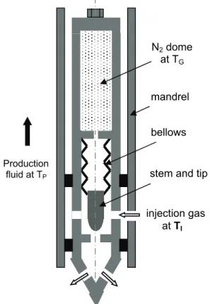
The production of an oil well usually occurs with the help of artificial lift methods. Among them, artificial gas lift is one of the most commonly used. A high pressure gas is injected in the annular gap between the well casing and the metal tube where the production fluid flows upward. A series of gas lift valves (GLV) are distributed along the tube and they serve as passages and as a means to control gas flow from the annular gap into the production fluid in the tube. The gas injected into the tube reduces the weight of the production fluid column and causes an increase of the well production. A GLV is usually located in a side pocket mandrel in the production tube, as indicated in Fig. 1, where it can be installed and retrieved when necessary, for repair or substitution. A very simple schematic view of an injection pressure operated GLV is presented in Fig. 2. It contains a nitrogen gas dome, connected by a small hole to a flexible bellows and to the valve stem and tip. Prior to installation, the GLV is charged with high pressure nitrogen, forcing the bellows to keep the valve in the closed position. When set in position in the side pocket mandrel and submitted to the injection gas pressure, the GLV bellows is forced upward and may eventually overcome the pressure of the nitrogen charge. In this case, the GLV stem tip lifts off the valve seat and the GLV opens. The GLV operation and control of the injection gas flow rate depends on the nitrogen charge pressure. This pressure is quite sensitive to temperature changes, so that the prediction of the nitrogen temperature is an important issue to the GLV operation.

Decker and Udell (1976) presented an analytical method to predict the pressure response of bellows operated valves. In their analysis, it depends on mechanical, thermodynamic and frictional factors, which were considered separately. The thermodynamic effects were related to the change of nitrogen pressure in the dome and they were investigated for isothermal and for adiabatic conditions, under a wide range of temperatures and pressures. Their results indicated that for nitrogen at high initial dome pressures, the pressure response is particularly sensitive to temperature changes. Winkler and Eads (1989) presented an accurate correlation for predicting the effect of temperature on the nitrogen pressure at the GLV dome. Their correlation is important to determine the nitrogen charge at the test rack, prior to the GLV installation, usually made at a temperature distinct from that in the well. It is evident from this work the need to predict the nitrogen temperature under the operating conditions in the well. Hassan and Kabir (1993) developed a model for predicting the flowing temperature of the annular gas and the mixture in the tubing as a function of both well

Paper accepted August, 2008. Technical Editor: Celso Kazuyuki Morooka

depth and production time. They considered simultaneously both the annular gas flow and the tubing production fluid flow for a continuous flow gas lift operation. It was indicated that a good prediction of the fluids temperatures is essential for the gas lift design, in particular for the bellows charged valves. This prediction would also be essential to evaluate the nitrogen charge temperature according to its position in the well. Assuming that the temperatures of the injection gas (TI) and the production fluid (TP) were known,

Bertovic et al. (1997) performed experimental tests and developed a model to predict the gas temperature (TG) in the valve dome. They

indicated that when the production fluid and injection gas temperatures are distinct, there is a potential uncertainty in the valve performance and its closing pressure.

T

T

Figure 2. Schematic view of the GLV in the side pocket mandrel.

A test facility was built and it was verified that the gas temperature in the valve dome (TG) was distinct from the injection

gas (TI) and the production fluid (TP) temperatures. A model to

estimate TG was given by the linear relation

P I

G 1 T T

T =( −α) +α (1)

In their analysis, the coefficient α depends only on the GLV geometry – it would be independent of the injection gas and production fluid temperatures. The tests were performed with a single GLV model, for which they found a constant value of α = 0.29. They indicated that distinct values of α might be obtained for other GLV. Shahaboddin et al. (2004) presented a numerical model to study the behavior of intermittent gas lift. Simulations were performed under various reservoir conditions, for different settings of the operational parameters. Heat transfer between the injected gas and the liquid slug was considered in their simulator. Their results showed that the accuracy of the model decreased if this heat transfer was ignored. An incremental technique used in this modeling allowed for detailed calculation of heat transfer and temperature gradient along the tubing, which affected all the properties of gas and oil. Their results indicated that the local temperatures of the injection gas and the production fluid are important parameters needed as inputs to the operation and control of a GLV in a well.

The purpose of the present work was to evaluate the gas temperature in the dome of a nitrogen-charged GLV as a function of the local injection gas and production fluid temperatures. The GLV model used in the present work was distinct from that tested by Bertovic et al. (1997), although both have the same manufacturer (Schlumberger, 2008). Thus, initially the heat transfer processes in the GLV were characterized, in order to evaluate the parameter α defined by Eq. (1). The work was performed in three stages. First, a compact thermal model based on estimated thermal resistances was developed to compare the axial and the radial thermal resistances

from the nitrogen in the GLV dome to the surrounding fluids. The purpose was to verify whether the injection gas temperature flowing in the valve lower end could affect the nitrogen temperature by conduction along the valve body. The second task comprised an experimental verification of the conclusions obtained from the compact thermal model. An experimental apparatus was built and thermal tests were performed with ambient air substituting the nitrogen charge in the GLV dome. In these tests, hot water replaced the production fluid, and compressed air at ambient temperature replaced the injection gas flow through the GLV. The laboratory test conditions were quite distinct from those in a production well, but the conclusions from the compact thermal model could be corroborated by the experiments. The third stage comprised a numerical analysis performed to simulate the radial and circumferential temperature distribution in the mandrel tube cross section around the GLV dome. The actual dimensions of the production tube with the mandrel walls around the GLV were considered in this analysis. The purpose of the numerical analysis was to obtain a correlation analogous to Eq. (1) for this valve.

N

dome

at T

mandrel

Nomenclature

A = mandrel surface area, m2

h = convective heat transfer coefficient, W/m2K R = thermal resistance, W/K

T = temperature, °C

Greek Symbols

α = dimensionless coefficient, Eq. (1)

θ = dimensionless temperature, Eq. (2)

ξ, η = coordinates on computational domain Subscripts

G relative to gas inside the dome I relative to injection fluid M relative to mandrel P relative to production fluid

S relative to mandrel surface around the GLV

Thermal Analysis

The compact thermal model analysis, the experimental investigation and the numerical simulations performed in the present work will be described next.

Compact Thermal Model

When the GLV is operating under steady conditions in the side pocket mandrel, the nitrogen gas temperature (TG) in the GLV dome

will be in the range between the production fluid (TP) and the

injection gas (TI) temperatures. In the radial direction, the GLV wall

surrounding the nitrogen dome is separated from the mandrel tube inner surface by a thin (around 1.4 mm) production fluid layer. The mandrel tube surfaces are in contact with both the production fluid and the injection gas, as indicated in Figs. 1, 2 and 7. The nitrogen in the GLV dome is in thermal contact, in the axial direction, with the production fluid at the topside and with the injection gas at its bottom. In the radial direction, the GLV dome is surrounded by a thin layer of stagnant production fluid and the inner surface of the side pocket mandrel tube. A compact thermal model equivalent to an electric resistances circuit was associated to evaluate the heat transfer between the nitrogen gas in the VGL dome, the mandrel tube and both surrounding fluids. In this investigation, the GLV was initially subdivided into several portions arbitrarily chosen and assumed isothermal. Inside the GLV, the conductive thermal resistances were evaluated by standard conductive axial and radial

stem and tip

bellows

Production fluid at TP

injection gas

wall resistances (Arpaci, 1966). This procedure required the GLV geometric dimensions and tabulated values of its materials thermal properties. The heat transfer coefficients needed to evaluate the convective resistances were approximated by typical values obtained from the literature (Kays and Crawford, 1993). The original thermal resistances circuit was reduced, by the association of series and parallel resistances, to a simple circuit where the node corresponding to the nitrogen temperature (TG) was connected to

three thermal resistances. At the other end, these three resistances were connected to nodes corresponding respectively to the mandrel tube (TM), the production fluid (TP) and the injection gas (TI)

temperatures, as indicated in Fig. 3. It should be emphasized that this analysis was based on an order of magnitude of the thermal resistances. The main purpose was to verify whether the injection gas temperature (TI) flowing through the GLV bottom could affect

the nitrogen gas temperature (TG) in the valve dome. In addition,

this rough analysis could also verify any preferable thermal path for the nitrogen gas heat transfer.

T

T

T

R

R

R

T

Experimental Investigation

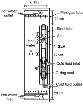
A thermal mockup of the actual GLV installed in the side pocket mandrel was assembled in the laboratory, assuming several simplifications, described as follows. The GLV actual operating conditions, mainly the high pressures of the injection gas and the nitrogen in the GLV dome, could not be reproduced in the laboratory. The experiments were performed with atmospheric air in the GLV dome and the injection gas was replaced either by compressed air or water flow at ambient temperature. The production fluid flow was replaced, in the thermal mockup,by an ascending hot water flow. Since in the experimental tests the air in the GLV dome was not pressurized, the GLV stem tip remained in the open position and the tests were performed with a steady flow of the injection fluid through the GLV. The main apparatus consisted of a GLV centered inside a carbon steel tube by two nylon sleeves with an O-ring seal in each one, as indicated in Fig. 4. The steel tube had a length of 600 mm and an inside diameter of 48 mm, with 6 mm wall thickness. The annular gap, around 5 mm, between the steel tube inner surface and the GLV outer surface was flooded by the hot water flow during the tests. The steel tube, with the GLV inside, was assembled against the inner surface of a vertical Plexiglas tube (150 mm inside diameter and 1000 mm long). Two disks, with a regular array of small drilled holes, were inserted at the bottom and the top of the Plexiglas tube to promote a uniform distribution of the hot water flow at these ends. As indicated in Fig. 4, two holes in the Plexiglas cylindrical wall provided the passages for the cold fluid inlet and outlet through the GLV. Thus, the cold fluid flow did not mix with the hot water flow during the experimental tests. The temperatures on several positions of the GLV, the steel tube, and both the hot water and injection fluid inlets and outlets were obtained from a total of 16 thermocouples made from type J, gauge 30 wire, distributed as shown in Fig. 4.

Figure 3. Equivalent thermal resistances of the compact model.

φ

Figure 4. Experimental apparatus.

There were eight thermocouples located around the air filled GLV dome, numbered from 1 to 8: two inside the dome, three on the GLV outer surface and other three on the outer surface of the steel tube surrounding the GLV. Thermocouples 9 and 10 were also located on the outer surface of the steel tube, at lower positions, as indicated in Fig. 4. Thermocouples 11 and 12 were located respectively at the GLV stem and tip. The remaining four thermocouples, 13-14 and 15-16, were used to measure respectively the cold and the hot fluid inlet and exit temperatures. The temperatures were recorded by a data acquisition system (a terminal bock, a multiplex amplifier and a data acquisition board, made by National Instruments) and stored in a microcomputer. A software (LabView) was used to display online the temperature readings on the computer monitor during each test. The uncertainty of the temperature measurements was estimated to be 0.5 oC.

Plexiglas tube

O-ring seal

GLV

Steel tube

Hot water

outlet

Hot water

inlet

Cold fluid inlet

20 cm

Cold fluid outlet

60 cm

Air

Hot

water

16

10 1

11 2 3 6

12 9

15 14 13 4

Numerical Analysis

The temperature of the nitrogen gas in the GLV dome is

infl at of the mandrel tube in the region

sur e. Since the mandrel tube surfaces are in

con

uenced mainly by th rounding the valve dom

Symmetry

line

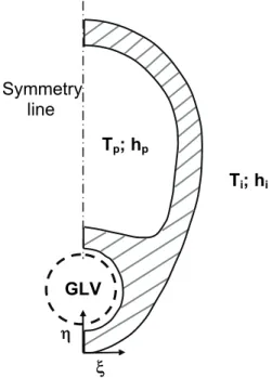
temperature distribution must be non uniform. Due to the mandrel tube geometry, the temperature distribution in its cross section surrounding the GLV dome was obtained numerically, using the CFD code Phoenics (CHAM, 2008), based on the control volumes method. It contains a facility called BFC (boundary fitted coordinates) to deal with irregular domains, which was employed in this analysis. Figure 5 illustrates a typical mandrel tube cross section at the GLV position, showing the thermal boundary conditions and the origin of the curvilinear coordinates ξ and η of the computational domain. Due to symmetry, the calculation domain for the conduction problem comprised only half of the mandrel tube cross section, as indicated in Fig 5. The boundary conditions at the interfaces with both the production and the injection fluids were convective. At the interface with the GLV, the mandrel tube surface was assumed adiabatic. Due to the absence of any heat source, the steady state mandrel tube wall temperature distribution was limited by the production fluid and the injection gas temperatures.

The temperature distribution in the mandrel tube wall was obtained in terms of a dimensionless wall temperature θ defined by

T

; h

T

; h

I P

I T T

T T

− − =

θ (2)

This dimensi

to 1 (production fluid). On the surface of the mandrel tube in contact with the production fluid, the convective heat transfer coe

Considering steady state operation, an electric resistances circuit

equ ated to the GLV geometry

and ces of the equivalent

elec

onless temperature varies from 0 (injection gas)

fficient hP was estimated from assumed flow rates in the range

from 50 W/m2_{.K to 350 W/m}2_{.K. On the outer surface, in contact}

with the injection gas, the heat transfer coefficient hI was obtained

from the ratio (hP/hI) in the range from 1 to 10. The numerical

results for the dimensionless temperature distribution in the mandrel tube were obtained using a total of 1200 control volumes in the domain indicated in Fig. 5, with essentially 20 nodal points in the η direction and 60 points in the ξ direction. The dimensionless temperature distribution θ was obtained numerically as

θ = θ(ξ, η, hP, hI) (3)

Compact Thermal Model Results

ivalent to thermal resistances associ materials was assembled. The resistan

tric circuit were then associated in series and in parallel, reducing the final circuit to that presented in Fig. 3. The thermal resistances indicated in Fig. 3 were estimated around RP = 600 K/W,

RM = 50 K/W and RI = 1000 K/W. These relative magnitudes

indicated that the injection gas temperature (TI) at the GLV bottom

practically would not influence the nitrogen gas temperature (TG) in

GLV dome. It also indicated that the strongest influence was that of the mandrel average wall temperature surrounding the nitrogen dome. Since these conclusions were obtained from estimated values of the thermal resistances and the associated thermal circuit, it was deemed necessary to verify them by an experimental investigation.

Figure 5. Cross section domain for numerical simulation.

Results

Experimental Results

The experimental tests of the thermal mockup indicated in Fig. 4 were performed under both steady state and transient conditions. Initially, a water flow at ambient temperature was forced upward in the Plexiglas vertical tube until all the thermocouples indicated a uniform temperature in the apparatus. Next, the water flow was electrically heated upstream of its entrance in the Plexiglas tube and, after a few minutes, the thermocouples inside the apparatus indicated a new thermal equilibrium at a higher uniform temperature. After this, a steady flow of compressed air or water at ambient temperature was forced through the GLV bottom, as indicated in Fig. 4, while the thermocouples readings were periodically recorded. Within a time interval of about ten minutes, there was a new equilibrium temperature distribution in the apparatus. The hot water and compressed air flow rates and inlet temperatures were constant during any test. Considering all the tests, the hot water flow rate and inlet temperature ranged respectively from 6 to 9 liters per minute and from 38 °C to 68 °C. In any test the hot water outlet temperature was always within 0.5 °C from its inlet temperature in the Plexiglas tube. The temperature difference between the hot water flowing in the Plexiglas tube and the cold fluid inlet in the GLV bottom was nearly constant during each test, from a minimum of 15 °C to a maximum of 45°C. Table 1 illustrates the equilibrium temperature distribution for the experimental test performed with the largest temperature difference. In this test the hot water temperature was around 68 °C and the injection compressed air was at 22 °C. The readings of thermocouples numbered 1 to 8 in Fig. 4, around the GLV dome, and those of the hot water (thermocouples 15 and 16) were within 1°C of each other.

ξ

η

Table 1. Experimental steady state temperatures.

Thermocouple T (°C) Thermocouple T (°C)

1 67.9 9 67.6

2 67.9 10 57.4

3 67.8 11 51.2

4 67.8 12 37.8

5 67.5 13 22.4

6 67.9 14 39.4

7 67.9 15 67.9

8 67.8 16 67.7

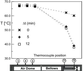
The temperature difference between the valve stem tip (thermocouple 12) and the dome region was around 30 oC in this test, indicative of a large thermal resistance along the GLV axis. The temperature distribution during the transient period of this test is indicated in Fig. 6. Initially just the hot water was forced upward in the Plexiglas tube until all the thermocouples indicated a thermal equilibrium. When the compressed air flow was forced through the GLV bottom, the resulting transient temperatures measured by five thermocouples positioned in the GLV are indicated in Fig. 6. Near the GLV dome, the temperatures remained almost uniform and steady. Near the valve stem base and tip, they decreased markedly with time, around 30 oC below the dome region temperatures, attaining a new equilibrium in about ten minutes. The dashed lines connecting the measured temperatures at identical time intervals are drawn just for clarity and are not intended to indicate a temperature profile along the GLV. The results from this and three other similar experimental tests indicated that the cold fluid injection at the GLV bottom practically did not affect the temperature in the GLV dome.

Although the hot water and the injection fluid temperature differences in the experimental tests were limited to about 45 °C, the results corroborated the predictions of the compact thermal model. In all experimental tests, the temperature inside the GLV dome was always determined by the mandrel tube temperature around the GLV dome. These results also suggested that the next step of this investigation should be a numerical analysis of the radial and circumferential temperature distribution in the mandrel tube surrounding the GLV dome.

Figure 6. GLV experimental transient temperature distribution.

Numerical Results

The dimensionless temperature distribution in the mandrel tube cross section indicated in Fig. 5 was obtained numerically, as described previously. The results depend on the position and the values of both heat transfer coefficients, as indicated by Eq. (3). To illustrate with an example, the temperature distribution for hP = 250

W/m2.K and hI = 50 W/m 2

.K is presented in Fig. 7. It indicates a non-uniform temperature distribution in the mandrel tube, ranging in this case from 0.67 to 0.80. As the heat transfer coefficients increased, the range of dimensionless temperature variation in the mandrel tube also increased – the maximum change of θ observed in one case was from 0.22 to 0.58. The circumferential dimensionless temperature distribution on the mandrel tube surface surrounding the GLV dome is denoted by θs, as indicated in Fig. 7. All the

performed numerical simulations showed that the θs distribution

ranged from the smallest to the largest calculated values of θ in the mandrel tube in each case. These results suggested a thermal model based on the assumption that the average temperature⎯θs was a good

estimate of the desired nitrogen gas temperature θG. This was

expressed by

) ,

( P I

s

G =θ =f h h

θ (4)

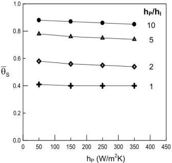
The effect of the convective coefficients on⎯θs is presented in

Fig. 8. There it is seen that this temperature is determined essentially by the convective coefficients ratio (hP/hI), suggesting a functional

relationship

) /

( _{P I}

s =f h h

θ (5)

30.0 40.0 50.0 60.0 70.0

Figure 7. θ-distribution on the mandrel tube cross section.

4 5 11 12

3

Air Dome Bellows

Δ

t (min)

0

5

12

T [

°

C]

0.2 0.6 1.0

0.0 0.4 0.8

1.0

Figure 8. Average temperature on the mandrel tube surface around the GLV.

Figure 9. Simplified thermal circuit.

The function defined by Eq. (5) was derived from an approximate thermal model considered next. Neglecting the mandrel tube radial wall thermal resistance, the magnitude of heat transfer from the production fluid to the injection gas through the mandrel cross section was characterized by the equivalent thermal circuit indicated in Fig. 9. From the solution of this circuit, the gas temperature TG can be expressed as in Eq. (1). The coefficient α,

which is equal to θG according to Eq. (2), can be evaluated by

) / ( )

/ (

) / (

I P I

P I

P _{f h h}

C h h

h h

= + =

α (6)

where C = AI/AP. Equation (6) was assumed to be a proper form to

correlate α to the ratio (hP/hI). In order to check this correlation, the

numerical results for⎯θs presented in Fig. 8 were rearranged in terms

of the ratio (hP/hI) and the parameter C in Eq. (6) was adjusted to fit

the numerical results. The results presented in Fig. 10 correspond to a value of C = 1.6. The correlation predicted the numerical results within 5% in the range of (hP/hI) from 1 to 10. It is worth to note

that the parameter C = 1.6 is close to the actual area ratio (AI/AP) for

typical mandrel tube cross section geometries.

Figure 10. Numerical results and the proposed correlating equation.

Conclusions

The present work was an effort to establish a correlation to obtain the nitrogen charge temperature in the dome of a GLV in terms of the local temperatures of the injection gas and the production fluid at the GLV location. A compact thermal model and an experimental investigation were initially performed in order to characterize the heat transfer between the GLV and the surrounding fluids. Both analyses indicated that the nitrogen gas temperature in the GLV dome was much more influenced by the radial heat transfer with the mandrel tube surface around the GLV than by the axial heat transfer along the GLV body. Numerical simulations were then performed to obtain the temperature distribution in the mandrel tube cross section around the GLV dome. The numerical results suggested a thermal model based on the assumption that the average temperature⎯θs was a good

estimate of the desired nitrogen gas temperature θG. From this, a

correlation based on the convective heat transfer coefficients hP

and hI was derived, in order to express the nitrogen gas

temperature (TG) in the GLV dome in terms of the production

fluid (TP) and the injection gas (TI) temperatures. The correlation

obtained in this work was related to a single retrievable GLV, but similar correlations could be obtained for other gas lift valves.

Acknowledgements

The authors gratefully acknowledge the support of Petrobras (Petróleo Brasileiro S.A.) and of CEPETRO-UNICAMP. We are also indebted to the engineers Galileu Paulo Henke Alves de Oliveira and Alcino Resende Almeida of CENPES-Petrobras, for bringing this problem to our attention and for their relevant support in the development of this work.

References

Arpaci, V.S., 1966, “Conduction Heat Transfer”, Addison-Wesley, US. Bertovic, D., Doty, D., Blais, R., and Schmidt, Z., 1997, “Calculating accurate gas-lift flow rate incorporating temperature effects”, SPE Production Operations Symposium, SPE 37424, 305-316, March.

Decker, L.A., and Udell, P.E., 1976, “Analytical methods for determining pressure response of bellows operated valves”, SPE Production Operations Symposium, SPE 6215, 1-38, October.

50 150 250 350 450

0 100 200 300 400

h

/h

10

5

2

1

h

(W/m

K)

θ

Numerical Results

6 . 1 ) h / h (

) h / h (

I P

I P

+ =

α

h

/h

α

0.6 0.7 0.8

0.0 0.1 0.2 0.3 0.4 0.5

0 1 2 3 4 5 6 7 8 9 10 11

(hA)

(hA)

Hasan, A.R., and Kabir, C.S., 1993, “Predicting Fluid Temperature Profiles in Gas-Lift Wells”, SPE 26098, 673-682, May.

Schlumberger, 2008, “Retrievable Gas Lift Valves”, respectively models Camco R-20 and Camco BK-1, in

http://www.slb.com/content/services/artificial/gas/rglv.asp. Kays, W.M., and Crawford, M.E., 1993, “Convective Heat and Mass

Transfer”, McGraw Hill. Winkler, H.W., and Eads, P.T., 1989, “Algorithm for more accurately

predicting nitrogen-charged gas-lift valve operation at high pressures and temperatures”, SPE Production Operations Symposium, SPE 18871, 415-422, March.