A. P. C. S. Ferreira
[email protected]A. R. de Faria
[email protected] Instituto Tecnológico de Aeronáutica – ITA Department of Mechanical Engineering CTA-ITA-IEM 12228-900 São José dos Campos, SP, BrazilSimultaneous Buckling and
Fundamental Frequency Optimization
of Frames under Uncertain Loadings
1
This work presents the optimization of a frame under uncertain loadings when two design criteria are taken simultaneously into account. The uncertainty relates to the applied loading and is inherent to the operation of structures since real structures are designed to sustain a large variety of load cases of practical relevance. The design criteria considered are two of the most important from a practical point of view: buckling load and natural frequency. The technique developed is based in convex modeling where a load space is defined and all the elements of that load space have equal probability of occurrence. The outcome of the technique is an optimal design for which one loading or several loadings of the load space are the most dangerous or harmful to the structure. On the other hand, it is guaranteed that all the other loadings contained in the load space are conservative in the sense that they are less harmful to the optimal design.
Keywords: multicriteria optimization, buckling, fundamental frequency, minimax strategy, uncertain loading
Introduction
Since there are hundreds or even thousands of load cases typically involved in practical structural design, one can admit that these load cases belong to a well-defined load space and then propose a strategy that optimizes the structure against the entire load space instead of a finite number of load cases. The proposed strategy would then be more conservative, because it would also subject the structure to loadings that were initially unspecified, i.e., that were not originally eligible load cases.
The optimization of buckling and fundamental frequency is a major concern in the aeronautical industry (Kim, Grandhi and Haney, 2006; de Faria and de Almeida, 2005; Wang, Jiang and Zhang, 2004; de Faria, 2002; Akgun et al., 2001; Liu, Haftka and Akgun, 2000). The goal is to get maximum buckling load and maximum fundamental frequency. However, there is a lack of efficient techniques capable of optimizing both simultaneously and in the presence of uncertainties. In general, it is very hard, and usually impossible, to find a single point (or variable) that simultaneously maximizes these two objective functions. A combination of two techniques is proposed. The minimax strategy (Banichuk, 1976; Dem’yanov and Malozemov, 1974) addresses the problem of uncertainty, whereas two possible techniques to be presented address the multiplicity of design criteria.
This work1 presents the optimization of a frame under uncertain loadings when two design criteria are taken simultaneously into account. The uncertainty relates to the applied loading and is inherent to the operation of structures since real structures are designed to sustain a large variety of load cases of practical relevance. The design criteria considered are two of the most important from a practical point of view: buckling load and natural frequency.
The technique developed in this paper is based in convex modeling where a load space is defined and all the elements of that load space have equal probability of occurrence. The outcome of the technique is an optimal design for which one loading or several loadings of the load space are the most dangerous or harmful to the
Paper accepted September, 2009. Technical Editor: Nestor A. Zouain Pereira 1
This material was previously presented as AIAA Paper 2008-5866 at the 12th AIAA/ISSMO Multidisciplinary Analysis and Optimization conference,
September 2008. Reprinted by permission of the American Institute of Aeronautics and Astronautics, Inc.
structure. On the other hand, it is guaranteed that all the other loadings contained in the load space are conservative in the sense that they are less harmful to the optimal design.
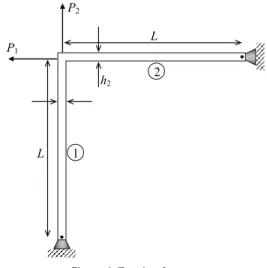
The uncertain loading representation discussed assumes its simplest form in the frame treated in this work and shown in Fig. 1. Two concentrated forces are applied simultaneously to the frame, but their magnitudes are assumed unknown and uncertain. The admissible load space in this case is spanned by these two concentrated forces through arbitrary linear, convex combinations.
L
L 1
2 P1
P2
h2
Figure 1. Two-bar frame.
Nomenclature
h = vector of design variables, m
K = stiffness matrix, N/m
KG = geometric stiffness matrix, N/m
l = number of individual initial stress states, dimensionless
M = mass matrix, kg
n = normal vector, dimensionless pi = loading parameters, dimensionless
p = global vector of applied loads, N Pi0 = loading scaling factors, N
q = displacement, m
Greek Symbols
δ = variational operator, dimensionless φ = auxiliary objective function, dimensionless λ = buckling load, dimensionless
λ0 = buckling normalization parameter, dimensionless
σ0 = initial stress state, N/m2 ω = fundamental frequency, Hz
ω0 = fundamental frequency normalization parameter, Hz ξi = nondimensional loading parameters, dimensionless
Subscripts
i relative to initial stress state
Problem Formulation
In problems related to the evaluation of buckling loads, the evaluation of the objective function is based on a prebuckling state and a linearized buckling problem that can be described in matrix form as:
p
KqP= , (1)
0 q K K− ) =
( λ G , (2)
where K is the stiffness matrix, qP are the prebuckling displacements, p is the global vector of applied loads, KG is the geometric stiffness matrix due to nonlinear displacements and q is the buckling mode associated with eigenvalue λ.
The modeling of problems related to the evaluation of natural frequency in the presence of stress stiffening effects can be described in matrix form as:
0 q M K
K− − ) =
( λ ω2
G , (3)
where matrix KG is linearly dependent on an initial stress state σ0. Therefore, if σ0 is represented by a linear combination of individual initial stress states, so is matrix KG. This linear combination is expressed in Eq. (4) considering that harmonic motion is possible.
0 q M K
K ⎟ =
⎠ ⎞ ⎜
⎝
⎛ −
∑
−=
2
1
ω ξ λ l
i i G i
, (4)
where l is the number individual initial stress states considered and
KGi is associated with the initial stress state σ0i such that:
∑
== l
i i i 1
0
0 σ
σ ξ . (5)
The nondimensional loading parameters ξi describe the contribution of σ0i to the vibration problem.
The two criteria, buckling and fundamental frequency are numerically computed by the finite element method. The Euler-Bernoulli beam theory is used to describe the structural behavior of a two-bar frame commonly referred to as Lee’s frame shown in the Fig. 1.
The Fundamental Frequency Surface
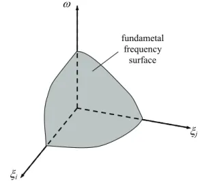
The fundamental frequency surface is used in this work as a means to visualize how the lowest natural frequency varies as the loading parameters ξi vary. A sketch of the fundamental frequency surface is shown in Fig. 2, where ω is the fundamental frequency. Notice that no constraint is imposed on the sign of the loading
parameters ξi. Moreover, depending on the initial stress state σ0i, the related geometric stiffness matrix KGi cannot be guaranteed to be positive-definite, although K and M are necessarily positive-definite.
fundametal frequency
surface
ω
ξ
iξ
jFigure 2. Fundamental frequency surface.
In order to investigate properties of the fundamental frequency surface, a perturbation analysis is conducted. Assume that the ξi ´s are slightly perturbed by δξi. The eigenproblem stated in Eq. (4) is perturbed accordingly:
0 q q q
M K
K
= + + +
× ⎥⎦ ⎤ ⎢⎣
⎡ −
∑
+ − + + +=
...) (
...) (
) (
2
2 2 2 2
1
δ δ
ω δ δω ω δξ
ξ λ l
i
i G i
i (6)
Subtracting Eq. (4) from Eq. (6), the first- and second-order equations can be written as
0 q M K K
q M K
= ⎟ ⎠ ⎞ ⎜
⎝
⎛ − −
+ ⎟ ⎠ ⎞ ⎜
⎝
⎛− −
∑
∑
= =
δ ω ξ λ
δω δξ
λ
2
1
2
1 l
i i G i l
i i G
i , (7)
and
0 q M K K
q M K
Mq
= ⎟ ⎠ ⎞ ⎜
⎝
⎛ − −
+ ⎟ ⎠ ⎞ ⎜
⎝
⎛ +
− −
∑
∑
= =
2 2
1
2
1 2
2
δ ω ξ λ
δ δω δξ
λ ω
δ
l
i i G i
l
i i G
i , (8)
Premultiplication of Eq. (7) by qT, and considering that M, K
and KGi are symmetric matrices yield
Mq q
q K q
T l
i i G i T
⎟ ⎠ ⎞ ⎜
⎝ ⎛ − =
∑
=1 2δξ λ
δω . (9)
where qTMq is certainly positive. However, the numerator in Eq. (9) may be either positive or negative. Premultiplication of Eq. (8) by
Mq q q M K K q T l i i G i
T λ ξ ω δ
δ ω
δ ⎟⎠
⎞ ⎜
⎝
⎛ − −
−
=
∑
=12 2
2 . (10)
The sign of δ 2ω2 is governed by the sign of the numerator in Eq. (10), since M is positive-definite and, therefore, qTMq > 0. Matrix
is positive semi-definite provided buckling
has not occurred, because, in this situation, )
( 2
1 K M
K−λ
∑
ξ −ω= l i i G i ) ( 1
∑
= − l i i G iKK λ ξ is
positive-definite. Therefore, from Eq. (10), it is concluded that δ2ω2
≤ 0, what proves that the fundamental frequency surface is concave. This property of the fundamental frequency surface is of utmost importance when it comes to optimization procedures.
The Stability Surface
Just as the concavity of the fundamental frequency surface was proved, it is possible to prove that the stability boundary surface is concave. Consider the buckling problem stated in Eq. (2) and define loading parameters pi = λξi such that the buckling problem can now be stated as
. (11)
1
0 q K K ⎟ =
⎠ ⎞ ⎜ ⎝ ⎛ −
∑
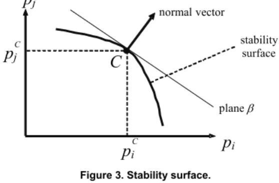
= l i i G i pAs ξi vary parameters pi also vary. This behavior can be visualized in Fig. 3 where the stability surface is shown along with other useful geometric entities. At point C, the vector normal to the stability surface can be seen as well as plane β tangent to the surface. Once ξiC and ξjC are available parameters piC and pjC can be obtained. Hence, in order to draw the surface presented in Fig. 3, one has to vary parameters ξi, evaluate the buckling load λ and compute parameter pi. This procedure results in a series of points, just like point C, that together compose the stability surface.
stability surface
p
jp
iplane β normal vector
p
iC
p
jC
C
Figure 3. Stability surface.
Consider now a point as close to point C as desired. This point has parameters piC + δpi + δ 2pi + … and pjC + δpjδ 2pj + … and its buckling problem reads
, ...) ( ...) ( 2 1 2 0 q q q K K = + + + × ⎥⎦ ⎤ ⎢⎣ ⎡ −
∑
+ + + = δ δ δ δ l i i G i ii p p
p (12)
where the superscript C has been abandoned. The first-order perturbation equation is, therefore,
0 q K q
K
K ⎟ =
⎠ ⎞ ⎜ ⎝ ⎛ − ⎟ ⎠ ⎞ ⎜ ⎝ ⎛ −
∑
∑
= = l i i G i l i i G i p p 1 1 δδ (13)
Premultiplication of Eq. (13) by qT and use of Eq. (11) lead to
0 1 = = ⎟ ⎠ ⎞ ⎜ ⎝ ⎛
∑
= n p q K q T l i i G i p δδ , (14)
where vectors n and δp are defined as
T l T l G T G T G T p p
p ... }
{ } ... { 2 1 2 1 δ δ δ δ = = p q K q q K q q K q
n . (15)
Equation (14) proves that vector n is normal to the stability surface. Consider now the second-order perturbation equation derived from Eq. (12):
. 1 2 1 2 1 0 q K q K q K K = ⎟ ⎠ ⎞ ⎜ ⎝ ⎛ − ⎟ ⎠ ⎞ ⎜ ⎝ ⎛ − ⎟ ⎠ ⎞ ⎜ ⎝ ⎛ −
∑
∑
∑
= = = l i i G i l i i G i l i i G i p p p δ δ δδ . (16)
Premultiplication of Eq. (16) by qT and use of Eq. (11) lead to
. (17)
1 2 1 0 q K q q K
q ⎟ =
⎠ ⎞ ⎜ ⎝ ⎛ + ⎟ ⎠ ⎞ ⎜ ⎝ ⎛
∑
∑
= = l i i G i T l i i G i T pp δ δ
δ
Premultiplication of Eq. (13) by δqT, recalling that KG i
are all symmetric matrices, leads to
. (18)
1 1 q K K q q K
q δ δ δ ⎟δ
⎠ ⎞ ⎜ ⎝ ⎛ − = ⎟ ⎠ ⎞ ⎜ ⎝ ⎛
∑
∑
= = l i i G i T l i i G i T p pSubstitution of Eq. (18) into (17) yields
0 2 1 = + ⎟ ⎠ ⎞ ⎜ ⎝ ⎛ −
∑
= n p q K K q T l i i G i Tp δ δ
δ , (19)
where
T l
p p
p ... }
{ 2
2 2 1 2
2 δ δ δ
δ p= . (20)
The first term in Eq. (19) is certainly nonnegative. Hence,
0
2
≤
n pT
δ . (21)
Equation (21) shows that the second order tangent vector to the stability surface, δ2p, and the normal vector n are orientated in opposite directions to each other. This can be visualized in Fig. 4. Therefore, from geometric arguments, it is concluded that the stability surface is concave with respect to the origin of the loading space pipj shown in Fig. 3.
stability surface
δ
pplane β n= normal vector
δ
2p
The concavity of both the fundamental frequency and the stability surfaces is of utmost importance when it comes to optimization procedures, as discussed in the next section.
Simultaneous Buckling and Fundamental Frequency
Maximization
Suppose it is required to maximize the fundamental frequency and buckling load obtained through solution of the eigenproblems given in Eqs. (4) and (11), respectively. In general, all the matrices involved K, M, KGi depend somehow on a vector of design variables designated by h. These design variables may represent a thickness distribution over plates or shells, fiber orientations in composite laminates, location of stiffeners in reinforced panels, etc. If the loading parameters are held fixed, one optimal design and corresponding fundamental frequency will emerge from the traditional optimization whereby the best h is selected. On the other hand, if the loading parameters vary, the optimal design for a given
h may not be optimal (and it may be in fact very poor) for another set of design variables h. In other words, the optimal design may be highly sensitive to variations in the loading parameters ξi.
The idea to eliminate, or at least alleviate, the sensitivity problem implies in the reformulation of the traditional optimization problem where the loading parameters are directly involved in the optimization process. The reformulation consists in proposing a bilevel optimization procedure where the fundamental frequency and buckling load are simultaneously maximized with respect to h
and minimized with respect to ξ = { ξ1ξ2 ... ξl }.
⎭ ⎬ ⎫ ⎩ ⎨ ⎧ =
= ⎭ ⎬ ⎫ ⎩ ⎨ ⎧
ξ
h
ξ
h h
h
ξ
h
ξ
h
ξ
h
ξ
h
, (
) , ( min ) (
), ( max ,
( ) , ( min max
λ ω φ
φ λ
ω
(22)
Function φ defined in Eq. (22) may appear redundant at first instance. However, the discussion about the properties of the fundamental frequency and stability surfaces presented in the previous sections will be extremely useful when it comes to the computation of φ.
Consider that a number of initial stress states can be applied to the structure. Each individual stress state has its own loading parameters ξi. These stress states are geometrically represented by dots in Fig. 5 on the ξiξj plane. Since the fundamental frequency and stability surfaces are both concave for a fixed design h, minimization of ω(h, ξ) and λ(h, ξ) with respect to ξ is simple, because the minimum is necessarily associated with one of the initial stress states on the polygonal dashed line drawn on the ξiξj plane. These initial stress states (on the dashed polygonal line) are said to be the convex hull of the set of all initial stress states. In Fig. 5, six out of thirteen initial stress states constitute the convex hull.
ω, λ
ξi
ξj
fundametal frequency or stability surface
Figure 5. Convex hull of initial stress states.
Since the fundamental frequency and stability surfaces are concave, every initial stress state that is given as a convex combination of the initial stress states belonging to the convex hull is guaranteed to yield a higher fundamental frequency or buckling load. The optimization procedure takes advantage of that property of the fundamental frequency and stability surfaces: when function φ is minimized with respect to ξ for ω or λ, it suffices to check for points on the convex hull and to select the worst among them.
One difficulty that appears is the fact that function φ corresponds in fact to a two-criterion objective function. Therefore, it is absolutely necessary to normalize ω and λ so that they are directly comparable. One practical approach is to check for design requirements and try to obtain target values for buckling loads and fundamental frequency and to use these as normalizing factors. Mathematically, if maximum buckling loads are available from design considerations f1, f2, …, fl and a fundamental frequency ω0 is also specified, then the normalized objective function should be used with λi* = λi / fi and ωi* = ωi / ω0. The optimal designs obtained following this procedure is dependant on the normalization factors f1, f2, …, fl, ω0. For instance, if ω0 is set too low, then the fundamental frequency criterion is expected to be unimportant, since ωi* would be high and probably one of buckling criteria λi* would be the dominant one. Hence, it is the designer’s task to select reasonable normalization factors. On the other hand, one of the advantages of the present strategy is its ability to detect such discrepancies in the normalization factors and to automatically improve those design criteria, which are the most vulnerable.
Numerical Results
The structure chosen for optimization is the so called Lee’s frame shown in Fig. 1. Its material is aluminum with Young modulus of 70 GPa and mass density of 2600 kg/m3. The two bar frame has rectangular cross-section with same width (b) and length (L), but different thicknesses (h). The length and width are constant and equal to 2 m and 1 cm, respectively. The thickness is the project variable, i.e., bar one has thickness h1 and bar two has thickness h2.
The concentrated forces are applied as shown in Fig. 1. Forces P1 and P2 are defined in Eq. (23):
20 2 2 10 1
1 P , P P
P =
ξ
=ξ
, (23)N 400 ,
N 800 )
2
N 800 )
1
20 20
10 20 10
= =
= =
=
P P
P P
P (24)
The loading parameters must be bounded such that a convex hull of the loading space is identifiable. In the present simulation, the relationship imposed on the loading parameters is
1 | | |
|ξ1 + ξ2 ≤ (25)
Since the fundamental frequency and stability surfaces are concaves, it is sufficient to evaluate λ and ω only at the surfaces vertices. That gives the following load cases:
1 , 0 ) 4
0 , 1 ) 3
1 , 0 ) 2
0 , 1 ) 1
2 1
2 1
2 1
2 1
− = =
= −
=
= =
= =
ξ
ξ ξ
ξξ ξ
ξ ξ
(26)
As buckling is associated to compressive loads and the fundamental frequency is lower when the frame is under compressive forces, only cases 3 and 4 are being considered. This, however, is not always true. For instance, in problems where shear loadings are important positive values of ξi should be considered. The frame is symmetric so it is expected that, for scaling factor 1 (P10 = P20 = 800 N) and load cases 1−2 and 3−4, buckling and fundamental frequency results behave symmetrically.
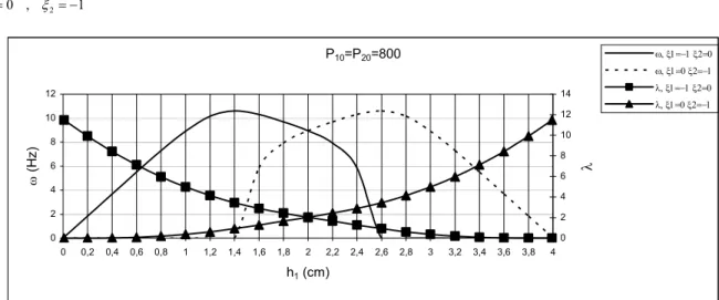
Considering that the frame’s total mass is constant, so that the two bar thickness sum is 4 cm (h1 + h2 = 4 cm), it is possible to visualize the buckling and fundamental frequency dependence on the thickness. Figure 6 shows how buckling and the fundamental frequency vary with h1 for P10 = P20 = 800 N and load cases 3−4. Figure 7 shows how buckling and the fundamental frequency vary with h1 for P10 = 800 N, P20 = 400 N and load cases 3–4.
P10=P20=800
0 2 4 6 8 10 12
0 0,2 0,4 0,6 0,8 1 1,2 1,4 1,6 1,8 2 2,2 2,4 2,6 2,8 3 3,2 3,4 3,6 3,8 4
h1 (cm)
ω
(H
z
)
0 2 4 6 8 10 12 14
λ
ω, ξ1=−1 ξ2=0 ω, ξ1=0 ξ2=−1 λ, ξ1=−1 ξ2=0 λ, ξ1=0 ξ2=−1
Figure 6. Two-bar frame fundamental frequency and buckling variation (P10 = P20 = 800 N).
P10=800 / P20=400N
0 2 4 6 8 10 12
0 0,2 0,4 0,6 0,8 1 1,2 1,4 1,6 1,8 2 2,2 2,4 2,6 2,8 3 3,2 3,4 3,6 3,8 4
h1 (cm)
ω
(H
z)
0 5 10 15 20 25
λ
ω, ξ1=−1 ξ2=0 ω, ξ1=0 ξ2=−1 λ, ξ1=−1 ξ2=0 λ, ξ1=0 ξ2=−1
Figure 7. Two-bar frame fundamental frequency and buckling variation (P10 = 800 N, P20 = 400 N).
In the context of multicriteria optimization, the fundamental frequency and buckling load should be normalized so that a proper comparison can be made. This work explores two normalization possibilities. The first one normalizes only the fundamental frequency (since the buckling load λ computed in this work is nondimensional) and uses as normalization parameter the lowest
frequency and buckling loads are better balanced. This region is named here as the optimal region.
Minimax Finding the Active Constraint
This approach takes advantage of the fact that buckling as used in this work (λ) is a nondimensional value and, therefore, only normalization of the fundamental frequency is required and can be done based on some lowest admissible frequency defined by project characteristics. Normalization of the fundamental frequency by the lowest admissible frequency (ω0) makes possible the identification of which restriction is active, that is, what criteria is dominant in the optimization process. In order to illustrate this point, two lowest frequencies will be adopted: ω0 = 13 Hz and ω0 = 3 Hz.
The minimax strategy is composed of two steps as described in Eq. (22). In the first step, thickness values are randomly generated (satisfying the constant mass constraint) and the corresponding buckling and normalized frequency values are computed. This results in two buckling and two fundamental frequency values. Among these four values, the lowest is taken as the solution φ(h) in Eq. (22).
The best design obtained from step 1 is taken as the starting point to the Powell’s method (Vanderplaats, 1984; Powell, 1964) in step 2. The objective function of this method is again φ(h) in Eq. (22b), so Powell’s method is employed to find the thickness that maximizes the minimum buckling and fundamental frequency. At the
end of this process the optimum thickness and the corresponding buckling and normalized fundamental frequency values are obtained. These are shown in Table 1 for P10 = P20 = 800 N. If the minimum among the buckling and fundamental frequency values corresponds, for example, to buckling, then it is said that buckling is the dominant criteria. The same hold for the fundamental frequency.
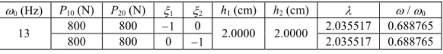
In Table 1, it is possible to see that frequency is the dominant criterion since it has the lowest value. Furthermore, it is shown that h1 = h2 = 2 cm is the best thickness configuration since it gives the greatest value among the minima. Fig. 6 can confirm this.
In Table 2, it is possible to see that frequency is the criteria dominant since it has the lowest value, furthermore, it is shown that h1 = 1.7155 cm and h2 = 2.2845 cm are the best thickness configuration since they give the greatest value among the minima. Fig. 7 can confirm this.
In Table 3, it is possible to see that buckling is the criteria dominant since it has the lowest value, furthermore, it is shown that h1 = h2 = 2 cm is the best thickness configuration since it gives the greatest value among the minima. Fig. 6 can confirm this.
In Table 4, it is possible to see that buckling is the criteria dominant since it has the lowest value, furthermore, it is shown that h1 = 1.6517 cm and h2 = 2.3483 cm are the best thickness configuration since they give the greatest value among the minima. Fig. 7 can confirm this.
Table 1. Active constraint for ω0 = 13 Hz and P10 = P20 = 800 N.
ω0 (Hz) P10 (N) P20 (N) ξ1 ξ2 h1 (cm) h2 (cm) λ ω / ω0
800 800 −1 0 2.035517 0.688765
13
800 800 0 −1 2.0000 2.0000 2.035517 0.688765
Table 2. Active constraint for ω0 = 13 Hz and P10 = 800 N, P20 = 400 N.
ω0 (Hz) P10 (N) P20 (N) ξ1 ξ2 h1 (cm) h2 (cm) λ ω / ω0
800 800 -1 0 2.616376 0.767070 13
800 400 0 -1 1.7155 2.2845 3.004458 0.767083
Table 3. Active constraint for ω0 = 3 Hz and P10 = P20 = 800 N.
ω0 (Hz) P10 (N) P20 (N) ξ1 ξ2 h1 (cm) h2 (cm) λ ω / ω0
800 800 -1 0 2.035517 2.984649 3
800 800 0 -1 2.0000 2.0000 2.035517 2.984649
Table 4. Active constraint for ω0 = 3 Hz and P10 = 800 N, P20 = 400 N.
ω0(Hz) P10 (N) P20 (N) ξ1 ξ2 h1 (cm) h2 (cm) λ ω / ω0
800 800 -1 0 2.765086 3.389255 3
800 400 0 -1 1.6517 2.3483 2.764997 3.243125
Minimax Finding the Optimal Region
This approach uses the minimax strategy to find the normalization parameters. The procedure starts applying the minimax strategy in the two criteria individually, which corresponds to solving Eqs. (27) and (28).
) , ( min ) (
) ( max ) , ( min max
0 0
ξ
h h
h
ξ
h
ξ
h
ξ
h
ω φ
φ ω
=
= (27)
) , ( min ) (
) ( max ) , ( min max
0 0
ξ
h h
h
ξ
h
ξ
h
ξ
h
λ ψ
ψ λ
=
= (28)
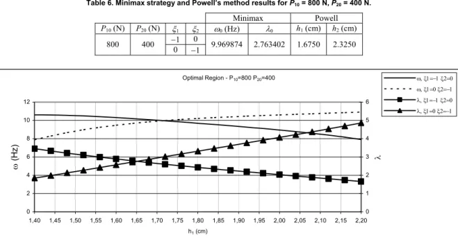
These values (ω0 and λ0) are used as normalization parameters in Powell’s method and define the region where the discrepancies in the optimization criteria are smaller. The objective function here is
again φ(h) in Eq. (22b), but the fundamental frequency and buckling values found in each step of Powell’s method are normalized by ω0 and λ0, respectively. Thus, Powell’s method is employed to find the thickness that maximizes the minimum normalized buckling and fundamental frequency.
Table 5. Minimax strategy and Powell’s method results for P10 = P20 = 800 N.
Minimax Powell
P10 (N) P20 (N) ξ1 ξ2 ω0 (Hz) λ0 h1 (cm) h2 (cm)
−1 0
800 800
0 −1 8.953811 2.035454 2.0000 2.0000
Table 6. Minimax strategy and Powell’s method results for P10 = 800 N, P20 = 400 N.
Minimax Powell
P10 (N) P20 (N) ξ1 ξ2 ω0 (Hz) λ0 h1 (cm) h2 (cm)
−1 0
800 400
0 −1 9.969874 2.763402 1.6750 2.3250
Optimal Region - P10=800 P20=400
0 2 4 6 8 10 12
1,40 1,45 1,50 1,55 1,60 1,65 1,70 1,75 1,80 1,85 1,90 1,95 2,00 2,05 2,10 2,15 2,20
h1 (cm)
ω
(H
z
)
0 1 2 3 4 5 6
λ
ω, ξ1=−1 ξ2=0 ω, ξ1=0 ξ2=−1 λ, ξ1=−1 ξ2=0 λ, ξ1=0 ξ2=−1
Figure 8. Two-bar frame fundamental frequency and buckling variation.
Conclusion
Structural projects are generally concerned with buckling and fundamental frequency optimization, and it is very important that the optimization of one does not harm the other. In this context, the demand for strategies capable of dealing with two criteria simultaneously is growing. The proposed strategy takes advantage of the fact that the interest is in maximizing these two criteria and reformulates the optimization strategy proposing a bilevel optimization procedure. Furthermore, the fact that the fundamental frequency and stability surfaces are concave represents a great reduction in the problem complexity and computational cost.
The multicriteria optimization needs ω and λ to be normalized for comparison purpose. This paper explores two distinct normalization ways. The first way permits one to identify which criteria is dominant in the optimization process. The second way permits one to define a region where the discrepancies in the optimization criteria are small.
The proposed optimization approaches proved satisfactory for the two bar frame under the load cases and scaling factors analyzed. This methodology can be applied in structural optimization problems with more than one project variable, like a two-bar frame with variable thickness or a plate. An important extension of this methodology is to include in the optimization a criterion that should be minimized, like compliance, and develop or apply a method capable of dealing with this kind of multicriteria optimization.
Acknowledgments
This work is financed by the Brazilian agencies FAPESP (grant no. 06/60929-0) and CNPq (grant no. 304060/2006-2).
References
Akgun, M.A., Haftka, R.T., Wu, K.C., Walsh, J.L., and Garcelon, J.H., 2001, “Efficient structural optimization for multiple load cases using adjoint sensitivities”, AIAA Journal, Vol. 39, No. 3, pp. 511-516.
de Faria, A.R., “Buckling optimization and antioptimization of composite plates: Uncertain Loading Combinations”, Int. J. Numer. Meth.
Engng, Vol. 53, Nov., 2002, pp. 719, 732.
de Faria, A.R., de Almeida, S.F.M., “The maximization of fundamental frequency of structures under arbitrary initial stress states”, Int. J. Numer.
Meth. Engng., Vol. 65, Aug., 2005, pp. 445-460.
Banichuk, N.V., 1976, “Minimax approach to structural optimization problems”, Journal of Optimization Theory and Application, Vol. 20, No. 1, pp. 111-127.
Dem’yanov, V.F., Malozemov, V.N., 1974, “Introduction to Minimax”, John Wiley & Sons, New York, Chap 3.
Kim, W., Grandhi, R.V., and Haney, M., 2006, “Multiobjective evolutionary structural optimization using combined static/dynamic control parameters”, AIAA Journal, Vol. 44, No. 4, pp. 794-802.
Liu, B., Haftka, R.T., Akgun, M.A., 2000, “Two-level composite wing structural optimization using response surfaces”, Struct. Multidisc. Optim., Vol. 20, Oct., pp. 86-96.
Powell, M.J.D., 1964, “An efficient method for finding the minimum of a function of several variables without calculating derivatives”, Computer Journal, Vol. 7, No. 2, pp. 155-162.
Vandeplaats, G., 1984, “Numerical Optimization Techniques for Engineering Design: With Application”, McGraw-Hill, New York, Chap. 3.
Wang, D., Jiang, J.S., Zhang, W.H., “Optimization of support positions to maximize the fundamental frequency of structures”, Int. J. Numer. Meth.