Carlos A. A. Carbonel H
[email protected]Augusto C. N. R. Galeão
[email protected] Lab. Nacional de Computação Científica – LNCC 25651-075 Petropolis, RJ, Brazil.A Finite Element Model for the Ocean
Circulation Driven by Wind and
Atmospheric Heat Flux
A finite element model for solving ocean circulation forced by winds and atmospheric heat fluxes is presented. It is vertically integrated 1 1/2 layer model which solves the motion and continuity hydrodynamic equations coupled with the advection-diffusion transport equation for temperature. A space-time Petrov-Galerkin formulation is used to minimize the undesirable numerical spurious oscillation effects of unresolved boundary layers solution of classical Galerkin method. The model is employed to simulate the circulation of the eastern South Pacific Ocean represented by a mesh covering the area between the equator and 30oS and between the 70oW to 100oW. Monthly climatological data are used to determine the wind and heat fluxes forcing functions of the model. The model simulates the main features of observed sea surface temperature (SST) pattern during the summer months showing the upwelling along the coastal boundary with currents oriented northwestward and the presence of southward flows and warm water intrusion in offshore side. The calculated SST fields are compared with the mean observed SST showing that the coastal processes and the interaction with the equatorial band are physically better resolved.
Keywords: ocean circulation model, stabilized finite element formulation, atmospheric forcing
Introduction
1
The finite element method using unstructured computational grids of triangular elements of variable size allows high resolution of local features in irregular domains. Consistent and stable weak formulation method lead to reliable accurate numerical schemes to solve the governing equations of the problem, allowing to rigorous integration of local and far-field interactions of the processes included in the mathematical formulation of the real problem.
The application of finite element methods in oceanography requires, as well, non-uniform refined mesh to take into account the irregular coastline shape. The spatial variability in grid spacing gives rise to unphysical wave scattering, which (under certain circumstances) could be of minor importance for steady state engineering problems, and to hydrodynamic problems at relatively short integration time; but might become of crucial importance as meso to large-scale ocean circulation modeling is focused. Besides, in ocean modeling, the numerical treatment of advection is still a very important issue, because the approximation of advection-dominated problems present numerical difficulties related to the lack of stability of the discretized operator.
There are several problems using finite element models for transient and convection dominated problems. When advection dominates diffusion, the classical Galerkin finite element methods generate unstable approximations, which usually exhibit spurious oscillations. Additionally, the models based on classical Galerkin formulations have shown some misbehavior in time-dependent propagation problems. Only for small values of the time integration step Δt it is possible to obtain numerical schemes that retain the high accuracy of the element-based spatial discretizations. For quite modest values of Δt, the accuracyand phase-propagation properties of the Galerkin formulation when applied to parabolic problems are lost, and the stability range is reduced in comparison with finite difference schemes (Donea and Quartapelle, 1992). In the case of hydrodynamic problems, it is more representative the features of the solution related to the accuracy/stability dependence on the dimensionless Courant number, instead of the size of the time step Δt.
Paper accepted September, 2009. Technical Editor: Francisco Ricardo Cunha
These disadvantages have motivated, in the last years, the development of alternatively finite element formulations such as Taylor-Galerkin, least-squares Galerkin and Petrov-Galerkin methods to improve the time-accuracy approximations of time evolution problems, particularly for those for which advection is the dominant behavior.
Finite element formulations based on the Streamline Upwind Petrov-Galerkin (SUPG) formulation and similar operators can solve the problem of unphysical wave scattering and unresolved boundary layer. These formulations were initially proposed for advection-diffusion and compressible flow problems (e.g., Brooks and Hughes, 1982; Shakib, 1988; Almeida et al., 1996). Formulations using a symmetric form of the shallow water wave equations were reported in last years (e.g., Bova and Carey, 1995; Carbonel et al., 2000). Also, for hydrodynamic baroclinic circulation, an approach was also presented (Carbonel and Galeão, 2006) focusing the wind-driven dynamic response in open and limited areas.
The ocean models range in dynamical complexity from simple linear surface–layer model to sophisticated, non-linear, continuously stratified systems. The physical inhomogeneous layers models were introduced by Lavoie (1972) and later important contributions using the same idea were published (e.g., Schop and Cane, 1983; Anderson, 1984; Anderson and McCreary, 1985; McCreary and Kundu, 1988; Ripa, 1993). The 1 ½-layer model presented here is the simplest possibility to represent physical processes in a real stratified ocean. The model has one active layer overlaying a quiescent, deep ocean, where pressure gradients are assumed to vanish. The water is allowed to move across the interface between the layers. The system is thermodynamically active so that the temperature in the upper layer changes its response according to the surface heat flux, the interface cooling flux, and the horizontal advection.
the use of artificial filters, mass diffusion and dampers, commonly used in several popular models. The treatment of the open boundary conditions is a very critical issue in a limited-area domain. For the model developed here, the treatment of the open boundaries is based on the formulation of weakly reflective open boundary conditions derived from the characteristic equations (Verboom, 1982; Verboom et al., 1983). The effectiveness of those kinds of boundary condition types for coastal circulation problems has been previously demonstrated (e.g., Carbonel, 2003; Carbonel and Galeão, 2006).
In the eastern ocean boundaries, the upwelling-favorable winds force offshore drift at the ocean surface, leading to upwelling of cold subsurface water at the coast, the formation and the offshore advection of coastal fronts, the generation of alongshore currents. Other commonly observed phenomena are the appearance of an equatorward surface jet, and a poleward undercurrent. In the present paper, the ability of the model to predict the above mentioned behavior is tested for the eastern South Pacific Ocean, focusing the simulation of the upper layer circulation and SST dispersion during the summer months. During this period the coastal upwelling remains weakly, but warming waters from the north invade the region, mainly in the offshore side. The simultaneously occurrence of colder waters near the coast and a southward warmer intrusion offshore configures a scenario with strong SST gradients, which is a challenger modeling ocean process in a limited area domain. The model is forced by monthly mean wind and solar radiation fields, but it develops its own fluxes of sensible and latent heat.
Nomenclature
AH, AV = horizontal and vertical eddy viscosity respectively, m 2
/s b = b=Tc /Tu, m/s
0
c = wave celerity, m/s
0
c = referential wave celerity, m/s
CS, CL = Stanton and Dalton parameters for the sensible heat and latent heat respectively
cpa = specific heat of the air, J/(kg o
C)
cp = specific heat of the surface water, J/(kg oC)
d = d=2c m/s
f = Coriolis parameter, sec-1 H = initial upper layer thickness, m He = depth scale of the entrainment process, m h = upper layer thickness, m
L = latent heat of evaporation, J/kg N = number of finite element sub-domains
k
P
= set of piecewise polynomials of degree ≤ kQ = net heat flux across the surface, Watt/m2
I
Q = heat flux across the interface, Watt/m2 Qs = net short wave radiation, Watt/m
2 Qlw = outgoing long wave radiation, Watt/m2
h
Q = sensible heat flux, Watt/m2
e
Q = latent heat flux, Watt/m2 q = saturation specific humidity R2 = the space of (x,y) points R± =Riemann invariant
n
S
= space-time finite element “slab” T = sea surface temperature (SST), oCTu = referential initial upper layer temperature, oC Tl =lower layer temperature, oC
te = time scales of the entrainment process, sec u, v = velocity components in the upper layer, m/s un = velocity component normal to the open boundary, m/s
U
nh = set of admissible trial functions
h n
Uˆ
= finite element subspace of weighting functions Vh = trial functionh
V
ˆ = weighting functionwed = entrainment-detrainment velocity, m/s
ω = divergence velocity, m/s xn = axis normal to the open boundary x, y = Cartesian coordinates
Greek Symbols
α = coefficient of thermal expansion, oC-1
ΓL = land type boundary ΓO = open ocean boundary.
πh , Δt
= pace time partition
e
Ω
= finite element sub-domainΩ
= spatial domainΓe = finite element boundary sub-domain
e
Ψ
= matrix of intrinsic time scaleϑT = thermal diffusivity, m2/s Φ = the empty set
ρair, ρu, ρl = densities of air, upper layer and lower layer respectively (kg/m3)
τ
x ,τ
y =wind stress components, N/m2The Ocean Model
The Governing Equations
We consider an incompressible fluid, which satisfies the Boussinesq approximation in a coastal ocean. An apparent temperature (Foffonof, 1962) is utilized and constant eddy coefficients are used to represent the turbulent exchange processes. Under these assumptions and defining a set of Cartesian coordinates (x, y, z) oriented positively to the East, North and upwards directions respectively, the governing equations describing the hydro-thermodynamical processes can be written as:
(
)
0 1 2 2 2 2 2 2 = − + − + − + + + z u A y u x u A x p fv z u w y u v x u u t u V H ∂ ∂∂ ∂ ∂ ∂ ∂ ∂ ρ ∂ ∂ ∂ ∂ ∂ ∂ ∂ ∂ (1)(
)
0 1 2 2 2 2 2 2 = − + − + + + + + z v A y v x v A y p fu z v w y v v x v u t v V H ∂ ∂∂ ∂ ∂ ∂ ∂ ∂ ρ ∂ ∂ ∂ ∂ ∂ ∂ ∂ ∂ (2) 0 1 = −g z p ∂ ∂ρ (3)
(
)
[
ref]
ref − T−T
=ρ α
ρ 1 (6)
In the preceding equations (u, v, w) are the velocity components in (x, y, z) directions respectively, t is the time and p is the pressure. ρ is the density and T is the apparent temperature with constant reference values ρref
and Tref respectively. The Coriolis parameter that depends on the geographical coordinates is represented by f and
g is the gravity acceleration. AH, AV and KH, KV are the constant horizontal and vertical eddy coefficients for momentum and temperature respectively and α is the thermal expansion coefficient.
The turbulent eddy viscosities and diffusivity constants are difficult to calculate accurately for oceanic flows, but some referential values could be considered for applications purposes (Stewart, 2004).
In the present paper we are mainly interested in the dynamical description of the upper layer ocean of density ρu
(x,y,t), thickness h
(x,y,t) and temperature T(x,y,t), overlying a deep inert layer of constant density ρl
and temperature Tl where the horizontal pressure gradients are set to zero. The lower layer is arbitrarily deep and its thickness Hl(x,y,t) is measured from a deep reference level up to the interface. The interface between these two layers represents the thermocline (see Figure 1).
Figure 1. The 1 ½ layer structure.
In a layered medium, boundary and interface conditions should be specified to close the system of equations governing the model behavior. For our particular model, let us introduce an interface level function η, such that η = Hl + h identifies the free surface, and η = Hl defines the common interface between the active upper layer and the inert lower layer. Under those assumptions the following set of conditions must be fulfilled:
x z H
z u A =−Υ
=η ∂ ∂ y z H z v A =−Υ
=η
∂ ∂
, =−Θ
=η ∂ ∂ z V z T
K (7)
ω ∂ ∂η ∂ ∂η η η η
η =∂∂ + = + = +
= t u x v y
w
z z
z 0 0
(8)
where ω is a vertical velocity due to mass transfer that should be zero at the free surface and equal to the entrainment-detrainment velocity wed at the interface between the upper and lower layers. At the free surface the heat source Θ = Q (the heat flux between the ocean and the atmosphere), and in the internal interface Θ = QI (the gain or loss of heat across this surface). The shear stress Υx , Υyare equal to the wind stresses (τx , τy) at the surface; and are assumed to be zero in the lower interface according to the proposed 1 1/2 layer model definition.
Integrating Eqs. (1), (2), (4), and (5), from the interface to the free surface, using the Leibnitz rule, and considering the boundary and kinematics conditions, we obtain
(
)
0 1 2 2 2 2 = − ∂ ∂ + ∂ ∂ − − + ∂ ∂ + ∂ ∂ + ∂ ∂∫
+ h ρ y u x u A fv dz x p y u v x u u t u u x H H h H u l l ∂ ∂ρ (9)
(
)
0 1 2 2 2 2 = − ∂ ∂ + ∂ ∂ − + + ∂ ∂ + ∂ ∂ + ∂ ∂∫
+ h ρ y v x v A fu dz x p y v v x v u t v u y H H h H u l l ∂ ∂ρ (10)
0 = − ∂ ∂ + ∂ ∂ + ∂ ∂ + ∂ ∂ + ∂ ∂ ed w y v h x u h y h v x h u t h (11)
(
)
1 02 2 2 2 = − + ∂ ∂ + ∂ ∂ − +
+ (Q Q)
h y T x T K y T v x T u t T I H ∂ ∂ ∂ ∂ ∂ ∂ (12)
Equations (9) to (12) describe the upper layer dynamics of the proposed 1 ½ layer model in a space time domain Ω x (0,T), where the spatial domain
Ω
⊂ R2 with land type boundary ΓL and an ocean type boundary ΓO such that ΓO∩ΓL=Φ(empty set) andΓO∪ΓL=Γ, the boundary ofΩ
.For simplicity, the same previous notation u, v, T is now being used to represent the mean horizontal velocity components and the mean temperature in this layer. For a generic variable φ(x,y,z,t), its mean value is:
dz h l l H h H
∫
+ = φφ 1 (13)
The vertical velocity wed which appears in Eq. (11), represents the entrainment-detrainment velocity given by
ed ed ed ed
ed (H h)H h/t H
w = − − (14)
where Hed and ted are the depth and time scale of the entrainment-detrainment process. This definition is similar to the entrainment equation proposed by McCreary and Kundu (1988). In the present case, the velocity wed avoids the interface from surfacing when (Hed –h) ≥ 0 and also avoids the interface from deepens excessively when (Hed –h) < 0. It is also possible to define a similar expression using different depths and time scales for the entrainment and detrainment (e.g., Roed and Shi, 1999).
According to Eq. (3), the pressure distributions in the upper layer pu and lower layer pl are given by
(
h H z)
g
pu=ρu + l− (15)
(
H z)
g gh
pl=ρu +ρl l− (16)
Using the anzatz
)] T T ( [ l l
u=ρ −α −
ρ 1 (17)
(
)
x T h x h g dz x p l l H h H ∂ ∂ μ θ ∂ ∂ σ ∂ ∂ ρ 21 = +
∫
+ (18)(
)
y T h y h g dz y p l l H h H ∂ ∂ μ θ ∂ ∂ σ ∂ ∂ ρ 21 = +
∫
+ (19)where μ=μ/(μ−σ),
μ
=ρ
u/ρ
l,σ
= 1 -μ
. Here, the influence ofthe salinity is not included, which does not mean a loss of generality, because an apparent temperature could be estimated modifying the constant α (Hantel, 1971; Fofonoff, 1962). The presented model is classified as an Inhomogeneous Layer Primitive Equations Model (ILPEN) valid for low-frequency dynamics (Ripa, 1993).
Forcing Functions, Boundary Conditions and Initial State
To completely define the proposed ocean model we need to characterize the applied external sources of energy, the time dependent boundary conditions and the initial state from which the relevant hydrothermodynamical response will be obtained.
The hydrodynamic behavior of the model is forced by the wind stresses evaluated from the wind velocity fields using the quadratic relations
W x D air
x ρ c W
τ = , τy=ρaircDWyW (20)
where
ρ
air is the air density and is the drag coefficient (Enriquez and Friehe, 1997). W(
0.509 0.065W)
/1000cD = +
x, Wyare the wind velocity components and |W| is the wind module.
The surface heat flux Q is the heat input at the ocean surface defined as
Q = Qsw - Qlw - QL - QS (21)
where Qsw is the net short wave radiation; Qlw the resultant outgoing longwave radiation; QS the sensible heat and QLthe latent heat. The sensible heat is calculated from the bulk formula
W ) T T ( C c
QS=ρair pa S − air (22)
where cpa is the specific heat of the air, CS an empirical coefficient, and T and Tair are the sea surface temperature and air temperature respectively. The latent heat is estimated from
W ) q q ( L C
QL=ρair L − air (23)
where L is the latent heat of vaporization, CL an empirical coefficient, and q, qair are the saturation specific humidity of the sea surface and air respectively. For a constant lower layer temperature
Tl the heat flux across the interface is given by: h / ) T T ( k Q l I
I = − (24)
showing that the gain or loss of heat across this interface, depends on the dynamical convergence or divergence of the flows ω in the upper layer, as expressed by the parameter kI =
ω
H(Carbonel, 2003). Concerning the boundary conditions it is assumed that land type boundaries give rise to the classical non-slip conditions:0 = =
v
u
(25)and for the upper thickness h and for the temperature T
homogeneous conditions are prescribed.
On the sea side boundaries, we prescribe a weakly reflective boundary condition, based on the characteristic method. This is done assuming that on a normal direction (xn) to the open boundary
0 = ± t d dR (26)
where the Riemann invariant R± = un ± 2c is valid along the characteristics dxn /dt = un ± c, normal to the open boundary. un represents the velocity component normal to this boundary and
h g
c=
σ
. The weakly reflective conditions on the open boundary are defined by the in-going characteristic of the presented equations. For the temperature at the open boundaries, homogeneous condition is assumed. Finally, the initial state requires the knowledge of a set of: initial velocity components( uo(x,y), vo(x,y) ); initial upper layer thickness ho(x,y) and an initial temperature field To(x,y), such that for
t = 0, u = uo, v = vo, h = ho, T = To in Ω (27)
A Quasi-Symmetric Form of the Governing Equations
Symmetric forms are always desirable because they possess better stability properties, an important feature to be used in the design of approximate solutions of advection dominated problems. For the particular case of fluid flow problems these aspects are pointed out in Shakib (1988), Almeida et al., (1996), Bova and Carey, 1995, Ribeiro et al. ( 1996). For the hydrothemodynamical problem treated in this paper a complete symmetrization is not achieved. Nevertheless, the hydrodynamic part of the equations governing the ocean circulation could be symmetrized. Furthermore, the whole set of unknown variables retains the same physical dimensions, which means that the transformed equations are adequately scaled.
This quasi-symmetrization is done introducing a new set of kinematic variables defined as:
h g c
d=2 =2 σ ,
u
T
T
c
b
0= (28)
which have the dimensions of velocity, and are function of the upper layer thickness h and the upper layer temperature T respectively. The parameter
c
0=
g
σ
H
is a referential celerity function of the referential initial upper layer thickness H and Tuis the referential initial temperature in the upper layer. After this change of variables, the set of equations for the unknown vector V = (u,v,d,b) could be written as:(
)
02 2 2 2 = + + + + +
+A V B V CV D V V F
V I y x y x t ∂ ∂ ∂ ∂ ∂ ∂ ∂ ∂ ∂ ∂ (29a) where
A= ,
⎟ ⎟ ⎟ ⎠ ⎞ ⎜ ⎜ ⎜ ⎝ ⎛ u u c u s c u 0 0 0 0 0 0 0 0 0
B= , (29b)
C= ,
⎟⎟
⎟
⎟
⎟
⎠
⎞
⎜⎜
⎜
⎜
⎜
⎝
⎛
−
0
0
0
0
0
0
0
0
0
0
0
0
0
0
f
f
D = , (29c)
⎟⎟ ⎟ ⎟ ⎠ ⎞ ⎜⎜ ⎜ ⎜ ⎝ ⎛ − − − H H H K A A 0 0 0 0 0 0 0 0 0 0 0 0 0 F= ⎟ ⎟ ⎟ ⎟ ⎟ ⎠ ⎞ ⎜ ⎜ ⎜ ⎜ ⎜ ⎝ ⎛
−Q h Q c g w -h ρ -h ρ -I e u y u x / ) (
, V= , ⎟⎟ ⎟ ⎟ ⎟ ⎠ ⎞ ⎜⎜ ⎜ ⎜ ⎜ ⎝ ⎛ b d v u
I = (29d)
⎟⎟
⎟
⎟
⎟
⎠
⎞
⎜⎜
⎜
⎜
⎜
⎝
⎛
1
0
0
0
0
1
0
0
0
0
1
0
0
0
0
1
and s=ghθTu 2μc0. The resulting equation system is an extension of the symmetric form of the hydrodynamic part of the model.
Space Time Petrov-Galerkin Method (STPG)
In this section we present the space-time Petrov-Galerkin finite element approximation for the continuous hydrothermodynamical ocean model described by Eq. (29).
We will assume that: the spatial region of interest is mathematically represented by an open bounded set
Ω
⊂ R2, with boundary Γ; and the time period of observation is the interval [0,ℑ]∈ R+. We now consider that for n = 0,1,2...M an ordered partition of time levels
t0 =0 < t1,...tn< tn+1...< tM= ℑ (30) is constructed. Denoting by In = (tn+1 - tn) the nth interval, we will say that, for each n, the space-time domain of interest is the “slab”
n
n
I
S
=
Ω
×
, with boundary Γn =Γ×In. Then for n = 1,2...N we will define a finite element triangulation of Ω such thatΩ
Ω =
∪
= e N
e 1 ;
Ω
i∩
Ω
j=
Φ
for i ≠ j; i,j=1,...N (31)In accordance with the previous definitions, we will assume that the finite element subspace is the set of continuous piecewise polynomials in , which may be discontinuous across the slab interface at t
h n
Uˆ
n
S
n , i.e.:
{
Vˆ ;Vˆ(
C( )
S)
;Uˆnh≡ h h∈ 0 n 4 Vˆ
(
P( )
S)
;Vˆ 0}
n e n h 4 e n k Sh ∈ =
Γ (32)
where is the set of polynomials of degree less than or equal to k. For a prescribed boundary condition
k n
P
h
V on Γn , a general trial function is then an element of
U
nh, where:{
V ;V(
C( )
S)
;Unh≡ h h∈ 0 n 4
(
k( )
ne)
4 h h}
S
h P S ;V V
V n e n = ∈ Γ (33)
For the present numerical ocean model, continuous interpolation in space and time will be adopted. Under this assumption, we will say that the approximate solution of Eq. (29) is the particular element Vh∈
U
nh, if it satisfies0
1
= Ω +
Ω
∑ ∫
∫
Vˆ d dt = h hd dtN e S h h S e n n R G Ψ
R e for n = 0,1,2 (34)
where
( )
( )
( )
( )
F D C B A I R + + + + + + = ) y V x V ( V y V V x V V t V V h h h h h h h h h h 2 2 2 2 ∂ ∂ ∂ ∂ ∂ ∂ ∂ ∂ ∂ ∂ (35)represents the residual associated to (29)
( )
( )
y Vˆ V x Vˆ V tVˆh h h h h
h ∂ ∂ + ∂ ∂ + ∂ ∂
=I A B
G (36)
is a space-time operator, and at the initial time
(
− 0)
Ω=0∫
V V VˆhdS h n Ω h
Vˆ
∀
(37)where V0 (Ω) is the initial condition in Ω.
The first integral appearing in Eq. (34) reproduces the classical Galerkin formulation whereas the integral under the summation index comes from the space-time Petrov-Galerkin formulation.
Ψ
e is the matrix of intrinsic time scales, containing free parameters, normally known as upwind functions (Hughes and Mallet, 1986). This matrix is symmetric and positive semidefinite and could be interpreted as an array of “scaling” parameters adequately chosen to “adjust” the weighting function effect. An optimal choice for Ψe is an open problem since convergence analysis and error estimates can provide some design conditions for Ψe, but are insufficient to determine an unique definition. Some procedures commonly used to estimate the intrinsic time scale matrix (e.g., Shakib, 1988; Bora and Carey, 1995; Ribeiro et al., 1996) do not give the best parameters for general applications in hydrodynamics and water waves. For these cases, some specific design procedures must be used to improve the physical and numerical mechanisms involved in practical problems.For complex system of equations, the Ψe definition is complicated due to the presence of multiple wave components. For the particular problem focused in this paper, we propose
( )
[ ]
[ ]
( )
12 2 2 2 2 1 1 ; h h e V V l t − ⎟ ⎟ ⎠ ⎞ ⎜ ⎜ ⎝ ⎛ ⎭ ⎬ ⎫ ⎩ ⎨ ⎧ + + Δ= I A B
Ψe (38)
where 1/le=
(
∂ξi/∂x)
max2 +(
∂ξi/∂y)
max2 is the representative length of the triangular spatial element , and are the local coordinates. Sincee
Ω ξi(i=1,2,3) e
Ψ
is symmetric, it may be computed in terms of its eigenvalues and eigenvectors, from the expansion∑
= = 3 1 k T k k k e γ e eΨ (39)
where ek are the eigenvectors and
are the eigenvalues. The intrinsic time scales components of the matrix Ψedefined in Eq.(38) will always be greater than Δt. The resulting system of algebraic equations is solved using the direct method of Gauss.
Numerical Results
A numerical experiment was conducted to evaluate the performance of the proposed discrete model to predict the main hydrothermodynamical features in a limited open region of the eastern South Pacific Ocean. The most familiar characteristic of eastern boundary ocean dynamics is the importance of equatorward surface currents and coastal upwelling resulting from a predominantly equatorward wind stress. The coexistence of countercurrents and undercurrents contributes to an even more complex dynamical behavior (Yoshida, 1967).
The region of interest (Fig. 2a) extends in the north-south direction from equator to the 30oS and in the east-west direction from the 70oW to 100oW. This region was discretized by an unstructured mesh of 5684 surface triangular elements and 2994 nodes, as illustrated in Fig. 2b. Near the coastline, a finer mesh was employed which gradually becomes coarser and coarser into the offshore region. The smaller element sides along the coastline are about 0.2o, whereas in the offshore left outer boundary they reach 0.9o.
(a)
(b)
Figure 2. The study area of the eastern South Pacific Ocean covers from the equator to the 30o
S and extend from the 70o
W to 100o
W; b) Finite element mesh of the study area in the eastern pacific coastal ocean.
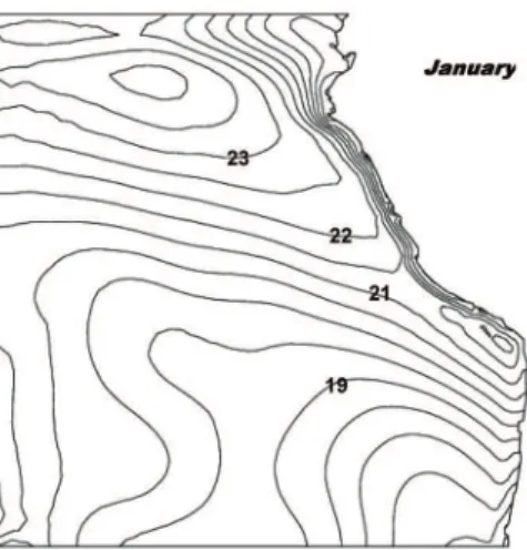
The model was forced at the surface by the monthly mean climatological wind velocity, net solar radiation (Qn = Qsw - Qlw ), the air temperature Tair, and the air specific humidity qair. These forcing data were extracted from the Atlas of Da Silva et al. (1994). It is necessary to remark that for the evaluation of the surface heat flux Q (Eq. 21), the contributions QSand QL were obtained using the water temperature T calculated by the model, instead of the observed monthly SST (Fig. 3). The discrete fields Qsw, Qlw,Tair, qair were obtained interpolating the original data at each node of the finite element mesh.
Figure 3. Horizontal monthly distributions of the observed sea surface temperature (o
C) during the summer months (from Da Silva et al., 1994). Contour intervals are 1oC.
The parameters of the model are mostly physically realistic values. The used densities of the upper layer, lower layer and air, ρu = 1022.5 kg m-3, ρl = 1025.5 kgm-3 and ρ
air = 1.1 kg m-3, respectively, are representative of the observed conditions in the region. The coefficient AH is 800m2s-1 and KH is 200m2s-1. The adopted entrainment-detrainment time scale ted = 1/4 day ensures that the upper layer thickness does not vanish in coastal upwelling areas, and also avoids the upper layer from becoming excessively thick in convergence regions.
In the literature, the parameters CL , CS used for the evaluation of the heat fluxes QLand QS range from 0.0008 to 0.002 (Bunker, 1976; Mc Creary et al., 1989; Kraus and Bussinger, 1994; Rosenfeld et al., 1994). Here, they were taken equal to 0.001. The specific heat of the air is cpa = 1004 J/kg. The saturation specific humidity q was evaluated in function of the saturation vapor pressure e (see Rosenfeld et al., 1994). The latent heat of evaporation was fixed equal to L = 2.44 x 10⁶ J/kg.The value of the coefficient of thermal expansion is α = 2.4 x 10³ o
C-1. The time step is defined as Δt = 3 hrs. The model response was started at rest in the month of January. The initial upper layer thickness was H = 50 m and the entrainment-detrainment depth Hed = 50m. The initial upper layer and lower layer temperatures Tu and Tl were taken as 28oC and 15oC respectively. The model was integrated forward for a period of 1 year using the monthly forcing functions from January to December, and the results shown in Fig. 4 to 6 correspond to the summer period of the second year.
Figure 4 shows the SST fields calculated by the model for the summer months (corresponding to end January, end February and end March). The resulting patterns of the temperature contours are similar to the observed ones.
The numerical solution shows colder waters (lower than 20oC), along the coastline and reaching also the southern offshore side of the region. This cooling process occurring in that region (from 20oS to 30oS) is not connected to a coastal upwelling phenomenon, but the cooling of the waters offshore is a consequence of the heat exchange fluxes between the atmosphere and the ocean dominated by the evaporation.
The calculated SST contour of 22oC clearly describes the evolution of the warm water intrusion observed in the data. The sequence of snapshots in the summer months shows the gradual advancing of the isotherm of 22oC to Southeast (January to February). During March, this 22oC isotherm returns to the north. The temperature contours show that the warm water intrusion reaches almost all the coast around the 20oS, diminishing the colder pattern in the sector comprising the 19oS to 25oS.
Figure 4. Horizontal monthly distributions of the calculated sea surface temperature (oC) during the summer months. Contour intervals are 0.5oC.
Figure 4. (Continued).
Figure 5 shows the calculated current fields during the summer months. A noticeable feature is the presence of an alongshore northward coastal jet associated with the coastal upwelling.
In the northern side (from equator to 5oS) a westward current is developed during January, reaching maximal values of 0.36 ms-1. This current weakens during February and March due to the weak winds and the reduction of evaporative cooling, leading to higher temperatures and owing to an unstable current pattern with the presence of southward flows. Note that a coastal countercurrent develops in the northeast. The southward flows are more intense in the west side of the study region.
Figure 5. Horizontal distribution of the calculated currents during the summer months.
Finally, to highlight the performance of the proposed model, we compare the calculated SST fields showed in Fig. 4 with the observed mean monthly SST fields presented in Fig. 3. Figure 6 shows the error fields (%). Note that in the region along the eastern boundary and the equatorial band, the relative errors are less than 5%.
The largest errors (greater to 15%) occur in small sectors of the model domain located in the northeast side (January) and in the southern side (February and March).
In general, the errors during the total period of integration were positive, indicating excessive cooling produced by the model.
The mesh used in the present section is adequate for the evaluation of the hydrothermodynamic study. A comparison of the results using three meshes were conducted and the results are presented in the appendix A.
Figure 6. Horizontal distribution of SST errors (%) of the model during the summer months. The error is defined equal to (Tobserved-Tcalculated)/Tobserved.
Conclusions
A 1 ½ finite element layer model for open and limited area domain is designed to describe the coupled hydrodynamic and thermodynamic processes of the surface layer of the ocean.
The numerical results obtained with this model for the hydrothermodynamics of the eastern South Pacific Ocean, during the summer months, are in a good agreement with the observed data. In particular, the occurrence of strong temperature gradients due to the intrusion of warm water to the south, and the presence of cool wind-driven coastal waters are well represented. Also, it is confirmed that the hydrothermodynamics of the upper layer in the studied region depends mainly on the interaction with the atmosphere. The relative errors are mostly less than 5% along the eastern boundary and the largest errors (~15%) occur in limited sectors.
These results indicate that the proposed model can be a useful tool to describe the most important transient circulation phenomena of the surface layer in the eastern South Pacific Ocean considering a limited area domain.
A numerical investigation of the annual cycle of the SST in this region is being prepared. Further implementation of the model with advective-diffusive equations of biological tracers will be of interest for marine biology.
Acknowledgments
This work was supported by normal fund of LNCC/MCT, FAPERJ/PRONEX. E26/171.199/2003 and by FAPERJ grant E-26/150.93/2007.
Appendix A
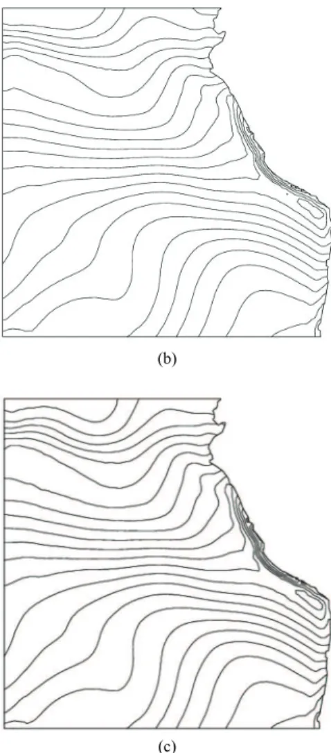
The influence of the mesh in the Hydrothermodynamic response is studied for three different discretizations. In Figure A1, it is presented the SST results for these three meshes. It is observed that for increasing number of nodes the SST get a similar pattern. For meshes with more than 2600 nodes the results show very small differences.
(a)
Figure A1. Calculated SST distribution at end March using: a) Mesh of 2369 nodes and 4455 elements b) Mesh of 2613 nodes and 4936 elements; c) Mesh of 2994 nodes and 5684 elements. Contour intervals are 0.5o
C.
(b)
(c)
Figure A1. (Continued).
References
Anderson, D., 1984, “An advective mixed layer model with application to the diurnal cycle of the low-level East African jet (Indian Ocean)”, Tellus – Series A, Vol. 36A, No. 3, pp. 278-291.
Anderson, D., McCreary, J.P., 1985, “Slowly propagating disturbances in a coupled ocean-atmosphere model”, Journal of the Atmospheric Sciences, Vol. 42, No. 6, pp. 615-629.
Bova, S.W., Carey G.F., 1995, “An entropy variable formulation and Petrov-Galerkin methods for the shallow water equations”. In: G.F. Carey (ed.), “Finite Element Modeling of Environmental Problems-Surface and Subsurface Flow and Transport”, John Wiley: London, pp. 85-114.
Brooks A.N., Hughes T.J., 1982, “Streamline upwind/Petrov-Galerkin formulations for convection-dominated flows with particular emphasis on the incompressible Navier-Stokes equations”, Computer Methods in Applied Mechanics and Engineering, Vol. 32, No. 1-3, pp. 199-259.
Bunker, A. F., 1976, “Computations of surface energy flux and annual air-sea interaction cycles of the North Atlantic Ocean”, Monthly Weather Review, Vol. 104, No. 9, pp. 1122-1140.
Carbonel, C.A.A.H., Galeão, A.C.N., 2006, “A stabilized finite element model for the hydrothermodynamical simulation of the Rio de Janeiro coastal ocean”, Communications in Numerical Methods in Engineering, Vol. 23, No. 6, pp. 521-534.
Carbonel, C.A.A.H., 2003, “Modelling of upwelling-downwelling cycles caused by variable wind in a very sensitive coastal system”,
Continental Shelf Research, Vol. 23, No. 16, pp. 1559-1578.
Carbonel, C., Galeão, A.C., Loula, A., 2000, “Characteristic response of Petrov-Galerkin formulations for the shallow water wave equations”,
Journal of the Brazilian Society of Mechanical Sciences, Vol. 22, No. 2, pp. 231-247.
Ribeiro, F.L., Galeão, A.C., Landau, L., 1996, “A space-time finite element formulation for the shallow water equations”. In: Proceedings of the International Conference on Development and Application of Computer Technics to Environmental Studies, pp 403-414.
Donea, J., Quartapelle, L., 1992, “An introduction to finite element methods for transient advection problems”, Computer Methods in Applied Mechanics and Engineering, Vol. 95, No. 2, pp. 169-203.
Enriquez, A.G., Friehe, C., 1997, “Bulk parameterization of momentum, heat, and moisture fluxes over a coastal upwelling area”, Journal of Geophysical Research, Vol. 102, No. C3, pp. 5781-5798.
Ripa, P., 1993, “Conservation laws for primitive equations models with inhomogeneous layers”, Geophysical and Astrophysical Fluid Dynamics, Vol. 70, No. 1-4, pp. 85-111.
Fofonoff, N.P., 1962. “Dynamics of ocean currents”. In: M.N. Hill (ed),
“The Sea, Vol. 1”, Interscience Publishers: New York, pp. 323-395. Rosenfeld, L.K., Schwing, F.B., Garfield, N., Tracy, D.E., 1994, “Bifurcated flow from na upwelling center: a cold water source for Monterey Bay”, Continental Shelf Research, Vol. 14, No. 9, pp. 931-939, 941-964. Hantel, M., 1971, “Zum Einfluss des Entrainmentprozesses auf the
Dynamik der Oberflachenschicht in einem tropisch-subtropischen Ozean”,
Deutsche Hydrographische Zeitschrift, Vol. 24, No. 3, pp. 120-137. Roed, L.P., Shi, X.B., 1999, “A numerical study of the dynamics and the energetics of cool filaments, jets, and eddies off the Iberian Peninsula”,
Journal of Geophysical Research, Vol. 104, No. C12, pp. 29817-29841. Hughes, T.J.R., Mallet, M., 1986, “A new finite element formulation for
computational fluid dynamics: III. The generalized streamline operator for multidimensional advective-diffusive systems”, Computer Methods in Applied Mechanics and Engineering, Vol. 58, No. 3, pp. 305-328.
Shakib, F., 1988, “Finite Element Analysis of the Compressible Euler and Navier Stokes Equations”, Phd. Thesis, Stanford University.
Kraus, E.B., Businger, J.A., 1994, “Atmosphere-Ocean Interaction”, 2nd
ed. Clarendon Press: Oxford, 362 p.
Stewart, R.H., 2004, “Introduction To Physical Oceanography Department of Oceanography”, Texas A & M University.
Lavoie, R.L., 1972, “A mesoscale numerical model of lake-effect storm”, Journal of Atmospheric Sciences, Vol. 29, No. 6, pp. 1025-1040.
Verboom, G.K., 1982, “Weakly-reflective Boundary Conditions for the Shallow Water Equations”, Delft Laboratory, Publication No. 26.
McCreary, J.P., Kundu, P.K., 1988, “A numerical investigation of the Somali Current during the Southwest Monsoon”, Journal of Marine Research, Vol. 46, No. 1, pp. 25-58.
Verboom, G.K., Stelling, G.S., Officier, M.J., 1983, “Boundary conditions for the shallow water equations”. In: M.B. Abbott and J.A. Cunge (eds.), “Engineering Applications of Computational Hydraulics, Vol. I”, Pitman Publ.: London.
McCreary, J., Kundu, P., 1989, “A numerical investigation of sea surface temperature variability in the Arabian Sea”, Journal of Geophysical Research, Vol. 94, No. C11, pp. 16097-16114.
Yoshida, K., 1967, “Circulation in the eastern tropical ocean with special references to upwelling and undercurrents”, Japan Journal of Geophysics, Vol. 4, No. 2, pp. 1-75.
Schop, P., Cane, M., 1983, “On equatorial dynamics, mixed layer physics and a sea surface temperature”, J. Phys. Oceanogr., Vol. 13, pp. 917-935.