A METHOD FOR COMPOSITE FAULT DETECTION AND ISOLATION
USING OVERLAPPING DECOMPOSITION
Rog´
erio Bastos Quirino
∗[email protected] md.cefetpr.br
Celso Pascoli Bottura
†∗Departamento de Tecnologia Eletromecˆanica, CEFET-PR. 85.884-000 Medianeira, PR, BRAZIL
†Laborat´orio de Controle e Sistemas Inteligentes, Departamento de M´aquinas, Componentes e Sistemas
Inteligentes, UNICAMP. P.O. Box 6101, 13083-970 Campinas, SP, BRAZIL
ABSTRACT
In this article, a method is developed for fault detec-tion in linear, stochastic, interconnected dynamic sys-tems, based on designing a set of partially decentral-ized Kalman filters for the subsystems resulting from the overlapping decomposition of the overall large scale system. The faulty sensors can be detected and isolated by comparing the estimated values of a single state from partially decoupled Kalman filters. The method is ap-plied to an example system with two sensors.
KEYWORDS: fault detection, overlapping, Kalman fil-ters, sensor failures, sensors.
RESUMO
Neste artigo ´e desenvolvido um m´etodo de detec¸c˜ao de falhas em sistˆemas dinˆamicos acoplados lineares e esto-c´asticos, baseado no projeto de filtros de Kalman parci-almente descentralizados aplicados aos subsistemas re-sultantes da decomposi¸c˜ao ”overlapping”do sistema glo-bal. A detec¸c˜ao da(s) falha(s) e o isolamento do(s) sen-sor(es) falho(s) s˜ao feitos atrav´es da compara¸c˜ao dos valores estimados dos estados redundantes dos filtros de Kalman parcialmente desacoplados. Um modelo de apli-ca¸c˜ao com dois sensores ´e utilizado na valida¸c˜ao do
m´e-Artigo submetido em 20/12/2000
1a. Revis˜ao em 3/6/2002; 2a Revis˜ao em 11/2/2003 Aceito sob recomenda¸c˜ao do Ed. Assoc. Prof. Liu Hsu
todo.
PALAVRAS-CHAVE: Detec¸c˜ao de falhas, decomposi¸c˜ao com sobreposi¸c˜ao, filtros de Kalman, falhas de sensores, sensores.
1
INTRODUCTION
An important problem facing engineers in designing complex industrial processes, which has attracted sci-entists and researchers in the field of systems science, is the problem of failure detection in running systems (Willsky, 1976 ; Isermman, 1984 ; Frank, 1990).
The failure detection problem is an extremely complex one, and the choice of an appropriate design depends heavily on the particular application.
An important issue to be considered by the designer of failure detection systems is the issue of computational complexity. One clearly needs a scheme that has rea-sonable time requirements. It would also be useful to have a design methodology that admits a range of imple-mentations, allowing a trade-off study between system complexity and performance.
SS1 x1,2 SS2 x2,2 SS3
Y1 Y2 Y3
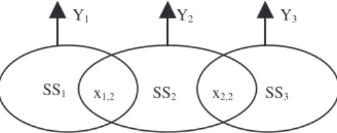
Figure 1: Overlapping decomposition for three subsys-tems.
We base this paper on the overlapping decomposition technique (Ikeda and Siljak, 1980) combined with a par-allel and distributed Kalman filter proposed in Quirino and Bottura, (2001) in order to yield a sensors multiple fault detection and isolation method.
A partially decoupled estimation methodology requires, when constructed, communication between the local fil-ters. In principle, such communication is in opposi-tion to the decentralizaopposi-tion philosophy of the overlap-ping technique. However, through this communication we achieve simultaneously two important aims: 1) The construction of a consistent estimator that complies with the detection structure; 2) The improvement of the per-formance of the detection system regarding its capacity to detect and isolate single faults as well as multiple faults.
The apparent contradiction that arises using distributed estimation techniques, developed in the two last decades and discussed in Quirino and Bottura (2001), jointly with the overlapping decomposition technique (Krtolica and Siljak, 1980), can have hindered progress in the de-velopment of methods for monitoring, distributed sensor fault detection and isolation.
Sensor Fault Detection (SFD) techniques for large-scale systems have been developed (Singh et al.,1983; Benkh-erouf and Allidina, 1987; Hassan et al., 1992), using an overlapping decomposition method.
This concept is accomplished (Ikeda and Siljak, 1980; Ikeda et al., 1981) by expanding the original system into a larger system comprised of a collection of intercon-nected subsystems. Although the order of the expanded system is higher than that of the original system due to the introduction of overlapping, the order of each sub-system (and consequently, the order of each one of the decentralized state estimators) is much lower. Further-more, it is only required that the subsystems be locally observable. This is easier to test for than the observ-ability of the original system.
In the method described by Hassan et al. (1992) state
observers for the interconnected subsystems are de-signed independently, neglecting the interaction terms between the subsystems.
The results obtained for suboptimal decentralized con-trol can be applied to the problem of decentralized state estimation (Krtolica and Siljak, 1980), by using duality.
It is thus possible to detect and identify a faulty sen-sor by comparing the discrepancies between estimates of the same (overlapping) state provided by different sub-observers. However, the sensor failures would only be detected and isolated correctly if they were assumed to occur one at a time.
In the following, we illustrate how a global system par-titioned into three subsystems with an expanded state space model in such a way as to generate two overlapped states.
Consider the case of overlapping decomposition for three partitioned subsystems, with two overlapped states x1,2 and x2,2 , as shown in Figure 1.
With respect to Figure 1, the rows of Table 1 show us each one of the ambiguous situations (column 1) be-tween simple (column 2) and multiple (column 3) faults, and the criterions (column 4) to them related. Such criterions (column 4) were established in Hassan et al. (1992) in order to treat uniquely simple fault (column 2) occurrences.
In this article we propose alternative criterions to those established in Hassan et al. (1992) , in order to avoid the ambiguity situations as shown in Table 1 and diagnose correctly simple faults as well as composite faults.
The use of the method developed by Hassan et al. (1992) would generate ambiguous situations and as con-sequences missed detections and false alarms. For exam-ple, in situation 4, as shown in Table 1, the composite failure of sensorsy1andy2, would produce a false alarm in sensory3and missed detections in sensorsy1 andy2.
In situation 1, as shown in Table 1, composite failure in all three sensors would not be diagnosed.
Thus, the SFD scheme proposed in Hassan et al. (1992) would fail to detect composite faults.
es-Table 1: Ambiguous situations for single and composite faults Sit. Single Faults Composite Faults Module of Estimation
Discrepances 1 no fault faults iny1,y2 andy3 |Z1,2|< ε1 and|Z2,2|< ε2 2 fault iny1 faults iny2 andy3 |Z1,2|> ε1 and|Z2,2|< ε2 3 fault iny2 faults iny1 andy3 |Z1,2|ε1 and|Z2,2|> ε2 4 fault iny3 faults iny1 andy2 |Z1,2|< ε1 and|Z2,2|> ε2 Z1,2= (χ1,2)SS1- (χ1,2)SS2;
Z2,2= (χ2,2)SS2– (χ2,2)SS3 ;
ε1, ε2 ≡constants to be determined.
(χ1,2)SSi≡estimate of the overlapped statex1,2 by the totally decoupled Kalman filter ofi-th subsystem.
(χ2,2)SSj≡estimate of the overlapped statex2,2 by the totally decoupled Kalman filter ofj-th subsystem. i= 1,2;j= 2,3.
timation structure. It is optimal in the sense of Kalman filtering and is based on the multiple projections (succes-sive orthogonalizations) method (Quirino et al., 1998).
The extension involves the use of a duality that exists between two state space representations.
It is derived from the application of an approach using the coupling and noise terms of the original system.
The algebraic structure developed is suboptimal, due to the fact that it does not take into account the updating of the state prediction based on the multiple innovations.
The article is organized as follows. Section two is con-cerned with the expansion and decomposition of a dy-namical system into a set of overlapping subsystems. The SFD procedure is described in section 3 and sim-ulations illustrating the method are given in section 4. Finally, some conclusions are given in section 5 .
2
SYSTEM MODEL AND
OVERLAP-PING DECOMPOSITION
Consider a large-scale linear interconnected system S, which is described by the following state and output equations:
S: xk+1=Axk+wk (1) yk=Hkxk+vk (2)
where x∈Rn, wk ∈Rn is the state noise vector, yk ∈ Rm is the output measurement vector and vk ∈ Rm is the noise disturbing the output. A and H are the system matrices of appropriate dimensions, in whichH is assumed to be a block-diagonal matrix withN blocks corresponding toN subsystems.
For the above system given by eqns. 1 and 2, we have
the following assumptions:
(1) wk and vk are Gaussian random vectors with zero mean and covariances respectively given byE{wjwt
k}= Qδjk ,E{vjvt
k}=Rδjk.
(2) The disturbance vectors are uncorrelated, i.e., E{vjwkt}= 0 ∀j, k.
(3) The initial state vector x(0) is a Gaussian ran-dom vector with mean E{x(0)} = X0 and covariance E{[x(0)−X0][x(0)−X0]t}=P0.
(4) x(0) and the noise vectorsvk and wk are uncorre-lated, i.e.,E{x(0)vtk}= 0, E{x(0)wkt}= 0 ∀k.
The systemSdescribed by equations (1) and (2) can be expanded into another systemS using a linear transfor-mation
xk=T xk (3)
wherex∈Rn(n >n) andT is an×n constant transfor-mation matrix. The expanded system is given by:
S : xk+1=Axk+wk (4)
yk =Hxk+vk (5)
wherewk is the expanded state noise andAand H are the new system matrices (with dimensionsn×n,m×n respectively) given by:
A=T ATI+M;H=HTI+L (6)
TI = (TtT)−1
Tt (7)
whereM and Lare complementary matrices of appro-priate dimensions (Ikeda and Siljak, 1980).
transformation matrix given by: T = I1,1 I1,2 I1,2 I2,1 . .. IN−1,1 IN−2,2 IN−2,2 IN,N (8)
whereIi,1is an identity matrix with dimension (ni-ni,2) × (ni-ni,2); Ii,2 is an identity matrix with dimension ni,2×ni,2, i=1,...,N.
3
FAULT DETECTION METHOD
In this section, we consider the problem of detecting the malfunctioning sensors of the augmented systemS, which comprises N overlapping subsystems. This will be achieved through the design of Partially Decentral-ized Hierarchical Kalman Filters (PDHKF), presented in Quirino and Bottura, (2001) for the subsystems and by comparing the estimated states, which are obtained by two successive filters for each subsystem.
Theith subsystemSiderived from the expansion is de-scribed by the following equations:
Si:xik+1=Aikxik+ N
j=1 i=j
Aijkxjk+wik (9)
yik=Hikxik+vki (10)
The results obtained for partially decentralized hierar-chical state estimation (Quirino and Bottura, 2001) can be applied by duality to the overlapping subsystems (9) and (10). The filters are designed as follows:
Consider the approximate equation for the expanded subsystemS
i:
Si:xik+1=Aikxik+ N
j=1 i=j
Aijkxjk+wik (11)
yik=Hikxik+vki (12)
where
wik= N
j=1 i=j
Aijkχjk+wik (13)
with χjk =xjk−xjk/k
By using (13) as a “plausible” approximation (Quirino and Bottura, 2001) to represent a white noise, we can es-timate the state xi
k+1, using a set of partially decoupled Kalman filters (Quirino and Bottura, 2001) described by the following stages:
Prediction Stage
xik+1/k=Aikxik/k+ N
j=1 i=j
Aijkxjk/k (14)
Pik+1/k =αik+1/kAikt+Qi
k (15)
where
αik+1/k =A i
kPik/k (16)
Qik =Qik+α ij
k+1/k (17)
αijk+1/k = N
j=1 i=j
AijPjk/kAijkt (18)
Qik Covariance matrix of thewik approximate expanded white noise;
Pik/k, Pjk/k Covariance matrices of the ith and jth ap-proximate expanded subsystems, respectively.
Correction Stage
xik/k =xik/k−1+Gikγk/k−1i (19)
where
Gik =Pik/k−1Hikt(HikPik/k−1Hikt+Rik)−1 (20)
denotes the gain matrices of the local Kalman filters and γk/k−i 1 is the measurement prediction error of the ith approximate expanded subsystem.
The covariance matrix ofxi
k/k , based onγk/k−1i can be written as:
Pik/k =KkiPik/k−1 (21) Kki =I−GikHik (22)
Due to the approximation (13), the prediction correction based on non local observations is unnecessary (Quirino and Bottura, 2001) .
Owing to overlapping decomposition, the state vec-tors xi and xi−1 share the part xi−1,2, i.e. , xi−1 = [xi−2,2
xi−1,1 xi−1,2
]tandxi= [xi−1,2 xi,1
Table 2: Sensor fault decision table for two sensors z1,2 Sensor fault decision
negative ≤ε fault iny1
>ε faults iny1 andy2
positive fault iny2
null normal operation
Let [xi−1,2k/k ]ss1 , [xi−1,2k/k ]ss2 represent the estimated val-ues of the state vectorxi−1,2 from the filters of subsys-temsi−1 andi, respectively.
For the case of two subsystems, during normal operation of the overall system we have
z1,2=E([x1k/k,2]ss1−[x1k/k,2]ss2) = 0 (23)
whereE is the mathematical expectance.
If one or more than one of theN subsystem sensors are malfunctioning, the above condition will be violated, as shown in Table 2.
As a result,Z1,2becomes biased (positive or negatively) because of the discrepance between estimates of the cor-responding overlapping state.
Thus, by examiningZ1,2 , the faulty sensors can be lo-calised as shown in the voting decision Table 2.
The tolerance value, ε, which is the magnitude of the departure from zero-mean, must be found for a specific application, depending on noise considerations and on model parameter uncertainty.
εis a constant which is usually determined by the experi-ence of the designer. However, in failure cases which are different from those considered in obtaining the value of ε, further investigation is required.
It is important to observe that such investigation can lead us to incorporate the failure estimation treatment into our proposal, due to the fact that different values ofεare useful in characterizing the failures.
The failure estimation problem involves the determina-tion of the extent of failure. This could be expressed by a sensor becoming completely non-operational(and be off or have hard-over failures), or by degradation in the form of a bias or reduced accuracy. The failures may be modeled as abrupt changes in the H matrix or as increase in the sensor covariance.
By inspecting the validity of eqn.(23), we can detect and locate the sensor failures among the N subsystems.
It is important to highlight that the use of decentralized
Approximate expanded system X2k/k= [ x1,2k/k x2,1k/k x2,2k/k]tO2
Failure Detection and Diagnosis : z1,2= E ( [ x1,2k/k ]ss1 - [ x1,2k/k ]ss2 ) 0 ?
Overlapping Observer SS1
Overlapping Observer SS2
Subsystem 2 Subsystem 1
y
1y
2P1k/k , X1k/k
P2k/k ,X2k/k
X1k/k= [ x1,1k/k x1,2k/k ]tO1
Decoupled Kalman Filters
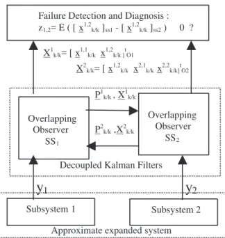
Figure 2: Approximate expanded system connected to failure detection system
estimation (14-22) modified the SFD scheme originally proposed in Hassan et al. (1992) (which uses differences between overlapping states of the subsystems), by the generation of different failure test conditions (Table 2). Another point to be noted is that in spite of not obtain-ing the best state estimate ofS, the unbias property is preserved, meaning that the scheme above will not only be useful as a composite fault detector but also as a good state estimator (by using the inverse of similarity transformation).
Figure 2 illustrates the use of the decentralized state estimators to detect faulty sensors when subsystemsS1 andS2 share the state variablex1,2.
Although the implementation of this SFD method re-quires communication between the subsystems, compos-ite faults are precisely detected and isolated and this enhances the reliability of the SFD scheme.
From the point of view of the sensor’s output, the sub-system estimators are completely decoupled, by the fact the state corrections are based on purely located obser-vations. In other words, such state corrections don’t take into account the successive orthogonalizations be-tween the subsystems. On the other hand, these es-timators take into consideration the interaction terms between the subsystems.
(i.e. strongly connected subsystems), a malfunction in any sensor could affect all the local filter estimates, and by consequence, compromise the response of the pro-posed SFD scheme.
Thus, it remains to show that the proposed SFD scheme also works satisfactorily in systems where the interac-tions may be strong, due to the fact the approximation (13) be just considered “acceptable” for weakly coupled systems (Quirino and Bottura, 2001).
In order to minimize the effect of noise, z1,2 is passed through a low-pass filter as follows:
z1,2(kf + 1) =zf1,2(k) +g.[z1,2(k+ 1)−z1,2(k)],f (24) where g is the filter gain. g and ε are chosen by sim-ulations. The gain g serves exclusively to smooth the estimator oscillations produced by the state and mea-surement noises.
In addition, if the state “Q” and measurement noise “R” covariance matrices, both diagonal, are such that the elements qii are identical for all i and rii are identical for alli, then a unique gain g will smooth all the state variables estimates simultaneously.
The filtered outputz1,2f is used to measure the departure of z1,2 from zero-mean, and thus to locate the faulty sensors.
4
APPLICATION AND SIMULATION
RE-SULTS
The results given in this section are obtained by consid-ering a 4th order system with two sensors outputs. By using an appropriate transformation matrix T and com-plementary matrices M and L, the approximate system is expanded into a 5th order system consisting of two interactive overlapping subsystems.
The actual parameter values used for the original 4th or-der system and the expansion obtained are given below:
Original System
xk+1=Axk+wk+c yk =Hkxk+vk
A=
0,18 0 0 0
−0,25 0,27 0 0
0,55 0 0,18 0
0 0,55 −0,25 0,27
ct=
4,5 6,15 2 2,65
H =
0 1 0 0 0 0 0 1
X0= [5 5 5 5];R= 10−3
I2;P0= 25I4;Q= 10−3 I4
Expanded Approximate System
xk+1=Axk+wk+c
yk =Hxk+vk
A=
0,18 0 0 0 0
−0,25 0,27 0 0 0
−0,25 0 0,27 0 0
0,55 0 0 0,18 0
0 0,55 0 −0,25 0,27
ct=
4,5 6,15 6,15 2 2,65
Q= 10−3
1 0 0 0 0 0 1 1 0 0 0 1 1 0 0 0 0 0 1 0 0 0 0 0 1
H =
0 1 0 0 0 0 0 1
P0= 25I5;R=R= 10−3 I2.
The overall system is split into two interconnected sub-systems, as shown by bold lines in A. The partially decentralized Kalman filters are calculated for the sub-systems.
A system simulation, which uses the matricesA, H ,Q andR of the approximate expanded original system is used to generate the measurementsy1 andy2.
Sensor faults are simulated as sudden changes in the ap-propriate elements of the measurement matrixH. The simulation results are obtained withg = 0.07 in equa-tion (24). In this applicaequa-tion,ε was taken to be equal to−0,6.
Case a: Normal operation. For this case, we have E([x1,2k/k]ss1−[x1,2k/k]ss2) = 0.
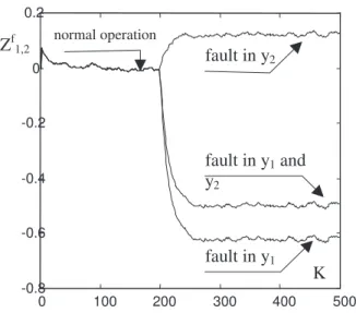
In this case, the matrix H is kept constant so that the simulated measurementsy1 andy2are the sen-sors outputs under no fault condition. The respec-tive estimates of the shared state are in very good agreement as can be seen from Figure 3 where the filtered differencezf1,2is shown. This indicates that both sensors are functioning normally.
In the following cases, failures of both sensors and of one sensor at a time are assumed to occur.
0 100 200 300 400 500 -0.8
-0.6 -0.4 -0.2 0 0.2
normal operation
fault in y
2Z
f1,2fault in y
1and
y
2fault in y
1K
Figure 3: Cases a, b, c and d of sensor faults
Case b: The sensor of subsystem 1 failed: (H1= [0 1.15]) at the iterationk= 200.
As result we haveE([x1,2k/k]ss1−[x1,2k/k]ss2)<0. The Figure 3 shows that, after the occurrence of the fault,z1f,2 becomes negatively biased which, ac-cording to the decision scheme in Table 2, indicates a fault in sensor 1.
Case c: The sensor of subsystem II failed: (H2= [0 0 1.15] ) at the iterationk= 200.
The filter results for this case (depicted in Figure 3) clearly indicate a positive deviation ofz1,2f from zero-mean, which corresponds to a fault in sensor 2.
Case d: Both sensors of the subsystems failed: (H1 = [0 1.15] and H2 = [0 0 1.15] ) at the iter-ation k = 200. Forε =−0.6 , in Table 2, these simultaneous faults are correctly detected by the filter as can be seen from the results in Figure 3.
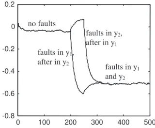
In figure 4, sequential failures of the sensorsy1and y2 are combined at the iterations k = 200 and k = 250. From the results in Figure 4, we can verify that the SFD scheme proposed will respond satisfactorily in diagnosing sequential failures, by the convergence of the single failure curves to that of the simultaneous failures situation shown in Fig-ure 3.
Since the filter calculations are performed on low-order blocks of subsystem equations, the SFD
pro-0
100
200
300
400
500
-0.8
-0.6
-0.4
-0.2
0
0.2
no faults
faults in y
1, after in y
2fault in y
2, after in y
1Z
f1,2K
Figure 4: Sequential faults
posed can work with accuracy and numerical sta-bility even for high-order systems.
Case e: Uncertainty in the parameters
In all the previous simulations, the partially decou-pled Kalman filters were provided with the exact expansion matrices and it was assumed that the system parameters are known exactly. In practice, there may be some uncertainty about the param-eter of the system and it is important to examine how this affects the SFD scheme.
To this end, the simulations performed in the cases of sequential and simultaneous faults are repeated with exactly the same conditions, except that the expanded matrixAused in the partially decoupled Kalman filtering scheme is perturbed in order to simulate parameter uncertainty, i.e., some of the parameters have been changed by more than 10%.
A=
0.16 0 0 0 0
−0.22 0.19 0 0 0 −0.25 0 0.24 0 0
0.45 0 0 0.1 0
0 0.5 0.56 −0.22 0.27
The PDHKF (Partially Decentralized Hierarchical Kalman Filter) results obtained are given in figures 5 and 6. It can be seen that the smoothed differ-ences Z1,2f have (non-zero) negative constant bias, even though there is no sensor fault.
0 100 200 300 400 500 -0.8
-0.6 -0.4 -0.2 0 0.2
faults in y
1and y
2K
fault in y
2no faults
fault in y
1Figure 5: Single and simultaneous faults with parameter uncertainty
figures 5 and 6. These results show a change to a different bias in Z1f,2 after the occurrence of each one of those faults.
Disturbances in the matrices Q, R, and P used by the PDHKF filter have also been simulated and sim-ilar results have been obtained (i.e.,Z1,2, depend-f ing on the fault locations, changes suddenly at some point in time, only when a sensor fault is present). Although the SFD scheme can cope with small pa-rameter uncertainty, robustness against larger un-certainty is an important consideration for practical applications and is the subject of current research.
5
CONCLUSION
In this paper, an extension of the Sensor Fault Detec-tion method introduced by Hassan et al.(1992) has been proposed. The objective of the extension was to detect and isolate precisely composite sensors malfunctioning. This is achieved by using an approximation which pro-vides estimated interactions between the subsystems as portions of system noise.
Suboptimal Kalman filters have been used to estimate the states of the overlapping subsystems and a proce-dure to incorporate new interactions within the filter equations has been described.
Simulation results using a low order system with two sensors have shown that the method operates satisfac-torily and that discrepances between estimates of the shared states of the subsystems can be used to identify
0 100 200 300 400 500
-0.8 -0.6 -0.4 -0.2 0 0.2
no faults
faults in y
2,
after in y
1faults in y
1,
after in y
2faults in y
1and y
2Figure 6: Single and sequential faults with parameter uncertainty
and precisely isolate malfunctioning sensors.
The method can be applied equally well to a large scale system decomposed into more than two overlapping sub-systems.
6
ACKNOWLEDGEMENTS
The authors wish to thank the reviewers for their thoughtful and helpful comments.
REFERENCES
Benkherouf, A., and Allidina, A.Y. (1987). Sensor fault detection using overlapping decomposition . Large Scale Systems, 12, pp. 3-21.
Frank, P.M. (1990). Fault diagnosis in dynamic systems using analytical and knowledge – based redundancy - A survey.Automatica, 26 (3), pp.459-474.
Hassan, M.F. , Sultan, M.A. , and Attia, M.S. (1992). Fault detection in large-scale stochastic dynamic systems. IEE Proc. D,Control Theory Appl., 139 (2), pp.119 –124.
Ikeda, M., and Siljak, D. D. (1980). Overlapping decom-positions, expansions and contractions of dynamic systems. J. Large-Scale systems,1, pp.29-38.
Isermann, R. (1984). Process fault detection based on modelling and estimation methods – A survey. Au-tomatica, 20 (4), pp. 387-404.
Krtolica, R., and Siljak, D.D. (1980). Suboptimality of decentralized stochastic control and estimation.
IEEE Trans. Autom. Control, AC-25, pp. 76-83.
Quirino, R.B. , Bottura, C.P., and Costa Filho, J.T. (1998).A computational structure for parallel and distributed Kalman filtering. Proceedings of the
XII Congresso Brasileiro de Autom´atica, pp. 747-753.
Quirino, R.B. , and Bottura, C.P. (2001).An approach for distributed Kalman filtering. Revista Controle & Automa¸c˜ao da SBA (Sociedade Brasileira de Au-tom´atica), Vol.12, No.1.
Singh, M.G. , Hassan, M.F. , Chen, Y.L. , and Pan, O.R. (1983). New approach to failure detection in large-scale systems . IEE Proc.D,Control Theory Appl.,
130 (5), pp. 243-249.