Progressivity of Personal Income Tax in
Brazil
∗
Horacio Levy
†
, José Ricardo Nogueira
‡
, Rozane Bezerra de Siqueira
§
,
Herwig Immervoll
¶
, Cathal O’Donoghue
k
Contents: 1. Introduction; 2. Income Tax Indexation and Inflation in Brazil; 3. Fiscal Drag and Distortions of the Tax Function; 4. Method; 5. The Brazilian Income Tax; 6. Income Tax and Inflation; 7. Conclusions.
Keywords: Income Tax; Inflation; Progressivity; Redistribution; Latin America, Brazil
JEL Code: H22; H23; C81.
Income tax reform in Brazil has mainly stressed changes in rates, aiming at increasing its progressivity. One aspect frequently overloo-ked is that, in the absence of adjustments of the tax rules to inflation, the level and distribution of the income tax burden can be substantially affected. We use a microsimulation model to simulate the potential re-venue and distributive effects of inflation on the income tax in Brazil. Our findings suggest that if the income tax is not adjusted for infla-tion, progressivity would decrease but redistribution would increase due to a larger tax burden, but income inequality would not substanti-ally change.
No Brasil, reformas do imposto de renda têm enfatizado mudanças nas alíquotas, objetivando o aumento de sua progressividade. Um aspecto fre-quentemente desconsiderado é que, na ausência de ajustamentos das regras do imposto em relação à inflação, o nível e distribuição da carga do imposto
∗A previous version of this paper was presented at the 1st General Conference of the International Microsimulation Association, Celebrating 50 Years of Microsimulation, August 2007, Vienna, Austria, hosted by the European Centre for Social Welfare Policy and Research. We would like to the Editor for useful comments on earlier drafts of the paper. Responsibility for any remaining errors is ours alone.
†ISER University of Essex, Colchester and ECV, Vienna. E-mail:[email protected]
‡Departamento de Economia, Universidade Federal de Pernambuco, Recife. Correspondence address: José Ricardo Nogueira, Departamento de Economia, CCSA, Universidade Federal de Pernambuco, Cidade Universitária, 50670-901 Recife-PE, (81) 2126-8378, Ramal 256. E-mail:[email protected]
§Departamento de Economia, Universidade Federal de Pernambuco, Recife. E-mail:[email protected] ¶OECD, Paris, ECV, Vienna, ISER University of Essex, Colchester and IZA, Bonn. E-mail:[email protected]
podem ser substancialmente afetados. Utilizamos um modelo de microssim-ulação para estimar os potenciais efeitos distributivos e arrecadatórios da inflação sobre o imposto de renda no Brasil. Os resultados sugerem que não ajustando o imposto de renda de acordo com a inflação, sua progressivi-dade diminui e seu efeito distributivo aumenta. Entretanto, a desigualprogressivi-dade de renda não muda significativamente.
1. INTRODUCTION
Since 1997, when the government abolished the existing automatic adjustment of the income tax1
schedule according to inflation, unions have pressed the government to readopt some regular indexing mechanism. However, the adjustments made in the last decade have been irregular. Only in 2007 a regular indexing regime was put in place, by which the income tax schedule is adjusted in accordance with the inflation target set by the Brazilian Central Bank. Thus, at the centre of the fiscal policy debate in Brazil are the effects of inflation on the personal income tax. A key issue involved is the distributional and revenue impact of the fiscal drag. This paper seeks to contribute to the debate by measuring the extent of that impact.
Few studies have attempted to analyze the distributive effect of the income tax in Brazil,2 one
main reason being the fact that the main data set used, the PNAD, does not contain direct information on income tax payments by individuals or families. To overcome this difficulty, we use a tax-benefit microsimulation model, BRAHMS, to investigate how inflation may affect the distributional features of the income tax in Brazil. This is done by simulating the amounts of income tax paid by individuals and families, using income and other relevant characteristics found in the micro data for Brazil. We take 2003 as the baseline. The analysis is performed for the period 2003-2008, with the nominal values of incomes and income tax parameters adjusted according to the inflation rate for each year.
Besides this introduction, the paper is divided in six sections. Section 2 gives some background information on the issue of income tax indexation in Brazil. Section 3 discusses the inflation-based distortions in the tax function induced by the presence of fiscal drags. Details about BRAHMS, the data used, the simulations performed, and the redistributive measures employed in the analysis are given in Section 4. Following on this, Section 5 reports the simulation of the distribution of income tax burden in Brazil and its progressivity for the 2003 baseline. In Section 6 we analyze how the impact of inflation on the nominal values of income tax payments affects the progressivity of the income tax. Finally, Section 7 presents the concluding remarks.
2. INCOME TAX INDEXATION AND INFLATION IN BRAZIL
Since the 1960s, when the government introduced an official mechanism of adjustment of monetary values known ascorreção monetária, Brazil has developed a large experience with indexation. For most policy analysts,3this process of generalized indexation gave rise, over the years, to a self-reproducing
inflationary process that was at the root of the hyper-inflation of the 1980s and early 1990s.4It is thus
not surprising that, after the successful economic stabilization plan enacted in 1994, policy makers have developed reluctance in resorting to statutory indexation.
1From now on, for convenience, we use the term income tax to refer to personal income tax. 2See, for example, Rocha (2002) and Hoffmann (2002).
This is reflected in the absence of a regular inflation-adjustment scheme for the personal income tax in the last decade. In fact, for six years, from 1996 to 2001, there was no adjustment of thresholds in the income tax schedule. Mainly due to pressure from trade unions and taxpayers there was some irregular adjustment between 2001 and 2006. The mounting public reaction to the infrequent adjustment of the personal income tax has also led the government to announce that for the period 2007 to 2011 the schedule is to be adjusted according to the Central Bank inflation target for that period, which was set at 4.5%.
Yet tax authorities in Brazil have argued that, besides fuelling inflation, the use of an automatic adjustment mechanism for the personal income tax schedule further reduces the (already small) number of taxpayers and the tax base through increases in the exemption limit.5
They argue that this tend to have a negative impact both on tax revenue and on theprogressivityof the personal income tax (Secretaria da Receita Federal, 2004).
On the other hand, taxpayers argue that the corrosive impact on disposable incomes, especially wages, of not adjusting the tax schedule by inflation is regressive. It is also frequent the perception among the population that irregular indexation has allowed the government to significantly increase income tax revenue.
Thus, there seems to be a conflicting view about the distributive and revenue effects of adjusting the income tax schedule by inflation between the Brazilian tax authorities and the general public. The former stressing the regressive impact of the adjustment and the potential revenue loss, the latter emphasizing the opposite view.
3. FISCAL DRAG AND DISTORTIONS OF THE TAX FUNCTION
Following Immervoll (2005), this paper focuses on the effect of inflation-induced distortions of the tax function.6
Let taxestbe a function of pre-tax incomey : t= t(y). Note that, while omitted here for conve-nience, other tax-relevant characteristicsz(such as family structure or employment status) will gener-ally enter the tax function. In a typical income tax system the tax function incorporates adjustmentsa
applied to pre-tax incomeyto yield taxable income (e.g. in the form of deductions), the tax rate sched-ules(.)as well as tax creditsc. Since bothaandcmay depend onywe havet(y) =s(y−a(y))−c(y). If not corrected, inflation erodes the real values of any nominally defined parameters ofs(.),a(.)and
c(.). The erosion of tax-bracket limits is perhaps the most obvious effect. The two factors determining to which extent inflation alters the real tax burden levied on a given pre-tax incomeyare the rate of inflation and the shape of the tax functiont(.).
How will the erosion of the real value of tax function parameters affect household incomes? On a theoretical level, Immervoll (2005) has shown that, while inflation-induced erosions of tax credits will always reduce liability progressivity, the effect is ambiguous as far as the erosion of deductions and tax bracket limits are concerned. In addition, theoretical conclusions about how inflation might affect progressivity in a nominally defined tax system are more difficult to arrive at oncecoraare functions ofy(as is, for instance, the case if earnings-related social contribution payments are tax deductible). In these cases, the results would depend both on the functional forms ofc(y)anda(y)and on whether and how these are distorted by inflation. In any case, if we are ultimately interested in how inflation affects the degree to which income taxes equalise net household incomes then results regarding liability progressivity are not sufficient. In addition one needs to know the size of tax burdens before inflation as well as the pattern of household sharing between tax units with different pre-tax incomes.
5The number of taxpayers in 2003 corresponded to about 6% of the economically active population (Secretaria da Receita Federal,
2004).
6For a detailed discussion on this and other channels through which changes in the general price level affect real tax burdens
Earlier empirical studies suggest a regressive nature of fiscal drag in the sense that, in relative terms, tax burdens increase by more for low-income groups than for high-income taxpayers. There have been studies for Australia (Taxation Review Committee, 1974), Canada (Vukelich, 1972, Jarvis, 1977), the USA ((Goetz and Weber, 1971, Von Furstenberg, 1975, Sunley and Pechman, 1976) and Italy (Majocchi, 1976, Lugaresi and Nicola, 1991). These studies also show that, in a progressive tax system, average tax rates increase for all income groups and that any discretionary adjustments of the tax schedule have generally less than compensated for the effects of inflation.
In his study of three European countries (Germany, the Netherlands and the UK), Immervoll (2005) has provided micro-based analyses of the effects of inflation-induced tax-burden changes on the distri-bution of household incomes. He found that, even during times of low inflation, effects on tax burdens can be substantial if no regularly applied mechanism exists whereby tax and contribution rules are inflation-adjusted. For all three countries, an erosion of nominally defined tax parameters was found to reduce overall tax progressivity but, as a consequence of increasing overall tax liabilities, enhance the equalising properties of tax systems.
4. METHOD
4.1. Model and data
Our analysis uses BRAHMS, the Brazilian Household Microsimulation System.7 BRAHMS is a
tax-benefit model that calculates personal income tax, social insurance contributions, social tax-benefits and disposable incomes for a representative sample of the Brazilian population. This is done by combining personal and household characteristics from each observation in the sample with detailed institutional information of the tax and benefit rules. The version of BRAHMS used here is 2003b. It relies on the data and the policy rules for the (baseline) year 2003.
Each tax and benefit is calculated in accordance to the legal system so that interactions between different policies are accounted for (e.g. tax deductibility of employees’ social insurance contributions). Income components that are not simulated (such as market incomes or pensions) are taken directly from the data. Any tax deductions, allowances and other provisions that depend on income, family situations or other characteristics recorded in the underlying micro-data are taken into account in the simulations.
BRAHMS’s version 2003b uses micro-data taken from the 2003 National Household Survey (Pesquisa Nacional por Amostra de DomicíliosPNAD). PNAD is the main socio-economic household survey in Brazil. The 2003 sample consists of 133,255 households and 384,834 individuals. The survey provides detailed information on socio-demographic and labour market information relevant for calculating tax burdens and benefit entitlements. For example, the survey distinguishes between workers who are and are not registered in the social security system or affiliated to a trade union. This information is crucial for taking into account tax evasion and to determine the eligibility to insurance benefits.
4.2. Simulation
INCOME TAX SIMULATION
In order to account for the large number of informal workers, income taxes and contributions simu-lated in BRAHMS are only computed for individuals who are registered in the social security or affiliated to a trade union. All other individuals reporting employment or self-employment income are assumed to belong to the informal sector and pay no taxes.8In fact, over 90% of all personal income tax in Brazil
7For more details on BRAHMS, see Immervoll (2005) and Immervoll et al. (2006).
is withheld at the source, which presupposes a formal work relation. Simulated contributory benefits are also conditional on membership in the social security scheme.
In 2003, all residents were required to file income tax returns if their taxable income exceeded an exemption limit equivalent to 4.4 times the minimum wage (MW).9Taxable income includes earnings,
property income, pensions and earnings-related contributory benefits.10 Maintenance transfers,
means-tested benefits and unemployment benefits are not subject to income tax. With a high degree of income inequality, a relatively generous exemption threshold, and the sizable informal sector, only about 6% of the economically active population pays income tax in Brazil
Personal income tax is levied at the individual level. However, taxpayers can also file jointly and ben-efit from a deduction (about 44% of MW) for each dependent relative.11There are also tax allowances for
public and private insurance contributions,12education (about 70% of MW for each dependent relative),
and medical expenses (subject to no limit), and for pensioners aged 65 or more of 4.4 MW. Alternatively, these itemised allowances can be replaced by a standard deduction equivalent to 20% of taxable in-come. The tax schedule consists of two bands. The marginal tax rate is 15% above the exemption limit and 27.5% for taxable income above twice the exemption limit.
Simulations in BRAHMS assume that individuals choose the tax and benefit options that maximise disposable income at the family level. Therefore, family members choose the taxation scheme (individ-ual or joint) and tax allowances that minimise the income tax liability of the family.
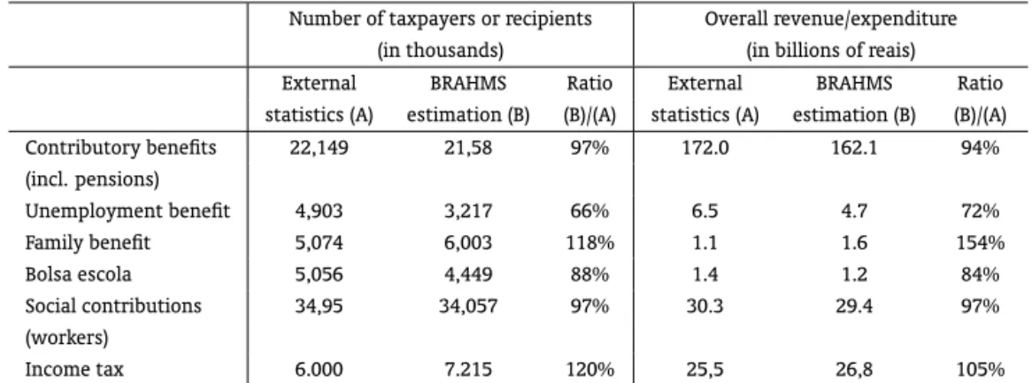
Comparisons of BRAHMS output against a number of official “headline” statistics are shown in Ta-ble 1. In general, the estimates compare reasonably well with availaTa-ble reference figures. Observed deviations are in line with those found for tax-benefit models in other countries and attributable to the data limitations and assumptions described above.13 More detailed validation-related data can be
obtained from the authors on request.
INFLATION ADJUSTMENT SIMULATION
One of the key advantages of the microsimulation approach is its ability to analyse one type of change (e.g., policy rules, incomes, personal characteristics, etc) at a time while holding “everything else” constant.14In the present study, this allows us to focus on the effects of inflation on the tax system
while keeping everything else constant (for example, changes in social contributions or in income due to other factors).
The effects of inflation on income tax are calculated by increasing all monetary variables in the micro-data in line with inflation, while using alternative hypotheses about inflation adjustment of income tax monetary parameters (e.g., thresholds in the tax schedule). In order to distinguish the effect on the income tax from that on other policies, all other simulated policies (i.e., benefits and social contributions) are also increased by inflation.15 Changes in real tax burdens can then be computed as
the arithmetic difference between the “before” (“baseline”) and “after” inflation scenarios. The analysis 9To facilitate interpretation, monetary values are expressed as a proportion of the national minimum wage (MW). In 2003, the
MW amounted to 240reaisper month, which corresponds to approximately 25% of the average wage. It is equivalent to US$ 129 in purchasing power parities.
10Investment income is subject to income tax, but withheld at the source and with different set of rates.
11These include spouses, children aged under 22 (or 25 when in education), and other relatives with taxable income below the
exemption limit.
12Public insurance contributions are deducted in full while private insurance contributions are deducted up to 12% of taxable
income.
13See, for example, the EUROMOD country reports onhttp://www.iser.essex.ac.uk/msu/emod/countries/. 14For an introduction to the microsimulation approach, see Redmond et al. (1998).
15Thus, the underlying assumption is that only income tax is not automatically and fully adjusted for inflation. In practice, social
Table 1: Numbers of recipients/payers and cost/revenue of benefits/taxes in 2003: BRAHMS simulations compared with external statistics
Number of taxpayers or recipients Overall revenue/expenditure (in thousands) (in billions of reais) External BRAHMS Ratio External BRAHMS Ratio statistics (A) estimation (B) (B)/(A) statistics (A) estimation (B) (B)/(A) Contributory benefits 22,149 21,58 97% 172.0 162.1 94% (incl. pensions)
Unemployment benefit 4,903 3,217 66% 6.5 4.7 72%
Family benefit 5,074 6,003 118% 1.1 1.6 154%
Bolsa escola 5,056 4,449 88% 1.4 1.2 84%
Social contributions 34,95 34,057 97% 30.3 29.4 97% (workers)
Income tax 6.000 7.215 120% 25,5 26,8 105%
Sources: OECD (2005), Ministério da Economia (2005), Ministério do Seguro Social (2005), and authors’ own elaboration using BRAHMS, version 2003b.
is thus static in nature as it does not attempt to capture any behavioural adjustments that tax units may consider in response to changing tax burdens. This should be kept in mind when interpreting results particularly when looking at the cumulative effects of inflation over longer periods of time.16
4.3. Measures of inequality, redistribution and progressivity
To measure the effects of inflation on the distributional properties of the tax system, we use a set of common inequality indicators and compare them17between a “before inflation” and “after inflation”
scenario. The inequality measures used are members of the so-called single parameter Gini (or S-Gini) family (Donaldson and Weymark, 1980, Yitzhaki, 1983). By choosing the value of an inequality aversion parameterv, the S-Gini (SG) allows different weightswto be put on the contribution of lower versus higher income groups to total inequality:18
SG(v) =
1 Z
0
w(p−L(p))dp (1)
where
w=v(v−1)(1−p)v−2, v >1 (2)
pis the rank of individuals in a population with individual observations ordered in ascending order of the variable (here income) whose inequality is to be measured andL(p)is the Lorenz curve,i.e., the share of total income earned by the poorestp.100%. Forv = 2, we havew = 2andSG(v)is the standard Gini coefficient of inequality where departures from equality(p−L(p))are weighted equally for allp, whilev >2(<2)gives more weight to smaller (larger)p.
index depends on negotiations between unions and the government, differing by union category). Private employee pensions, other than the minimum pension, are readjusted by inflation.
16However, in subsection 6.3 below, we discuss some of the likely behavioural effects of inflation.
17The analysis does not, therefore, consider the inter-temporal redistribution mechanisms built into social insurance schemes. 18See, e.g., Duclos and Araar (2006). A stimulating discussion of alternative interpretations of Gini coefficients is provided by
Choosing an appropriatev, one can rank different distributions (e.g. before- and after-tax incomes) in terms of inequality or, alternatively, find the inequality aversion parametervwhere rankings change. For empirical applications, it is therefore desirable to find intuitive interpretations of differentvvalues. In principle, and as demonstrated by Blackorby and Donaldson (1978), relative inequality indices can be linked to a particular social evaluation function. For the S-Gini, a simple method for determining useful ranges ofv is presented by Duclos (2000). Consider Okun (1975) “leaking bucket” experiment where a hypothetical transfer from a richer person to a poorer person involves some efficiency loss in the sense that the gain enjoyed by the recipient is less than the loss suffered by the donor. Linkingv
to this efficiency loss, it is possible to derive, for a givenv, the implied fraction of the transfer that can be “lost” in the process while still making the transfer socially desirable. Choosing these amounts of tolerable wastage is perhaps more feasible or, at least, more intuitively appealing than directly deciding on an appropriate value ofv. For rank-preserving transfers from a person with rankp1 = 0.67to a
person with rankp2 = 0.33it turns out that withv = 2, the implied tolerated wastage amounts to
50% of the transferred amount. Withv= 1.5the amount would be only 29% and withv= 3a rather high 75% so that a transfer would still be judged desirable if only a fourth of the amount paid byp1
reaches the recipientp2.19 In the analysis that follows, we will present results for these three values of v.
The difference between the S-Gini index of inequality of pre-tax incomeSGgand the S-Gini
concen-tration index of net incomeCInis a measure of vertical redistribution. It indicates to which extent net
incomes are more equally distributed than gross incomes and, forv= 2, corresponds to the well-known Reynolds-Smolensky redistribution indexRS(Reynolds and Smolensky, 1977)
RS=SGg2−CIn(2) = 2
1 Z
0
p−Lg(p)dp−
1 Z
0
p−Cn(p)dp
(3)
whereLg(p)andCn(p)are, respectively, the Lorenz and concentration curves of before- and after-tax
income. If the tax function incorporates characteristics other than income, then income units may have a different order of incomes before and after the operation of the tax system. For example in Brazil the income tax allowance for pensioners aged 65 or more will cause these pensioners, after the operation of the tax, to shift up the distribution relative to younger individuals with the same pre-tax income. If non-income characteristics are judged irrelevant, re-ranking can be regarded as an indication of horizontal inequity and thus reduces the equalising effect of the tax. In this case the redistributive effectREof a tax is better measured as the difference between the pre- and post tax S-Gini indices of inequality, which captures the effect of re-ranking, expressed by the termd, on vertical redistribution:
RE =SGg(2)−SGn(2) =RS−d (4)
The inequality reducing properties of a tax depend on the inequality of the distribution of tax bur-dens as well as their size. Formally, it can be shown that
RE =k r
1−r −d (5)
where
r=(µg−µn) (µg)
(6)
19Givenv, tolerable efficiency losses increase with the rank difference of the two individuals. For
k= 2
1 Z
0
p−Ct(p)dp−SGg(2) (7)
d=SGn(2)−2
1 Z
0
p−Cn(p)dp (8)
and ris the size of the tax instrument expressed as the relative difference between mean gross and net incomesµg and µn,k is the Kakwani progressivity index (Kakwani, 1977), anddis the
above-mentioned re-ranking term measuring by how much vertical redistribution is reduced as a result of differences in the ordering of gross and net incomes (Atkinson, 1980, Plotnick, 1981).20 C
t(p) and
Cn(p)are, respectively, the cumulative proportions of total tax burdens and net incomes at point p
where individuals are ordered in terms of gross incomes. Since the decomposition works analogously for
w6= 2, we can derive measures of redistribution (RE) and progressivity (k) using different inequality aversion parametersv.
5. THE BRAZILIAN INCOME TAX
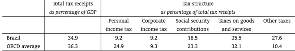
Although usually at the centre of the tax policy debate in Brazil, the share of the personal income tax on the overall tax revenue is smaller than in other countries. Table 2 shows that despite a similar total tax burden, as a proportion of GDP, the revenue derived from personal income taxation in Brazil is much lower than in the OECD average.
Table 2: Taxation in Brazil and in the OECD: 2003
Total tax receipts Tax structure as percentage of GDP as percentage of total tax receipts
Personal Corporate Social security Taxes on goods Other taxes income tax income tax contributions and services
Brazil 34.9 9.2 9.2 18.5 35.5 27.6
OECD average 36.3 24.9 9.3 23.3 32.1 10.4
Sources: Ministério da Economia (2005), OECD (2005) and OECD (2006).
Tax-benefit microsimulation allows us to go beyond aggregates and learn more about how the in-come tax is distributed. Table 3 reports the distribution of simulated inin-come tax liabilities as a propor-tion of total income tax revenue and as a proporpropor-tion of household disposable income. These figures relate to the simulation of the 2003 tax-benefit rules on 2003 data from the PNAD. Throughout the pa-per this simulation is taken as a “baseline”. According to the simulation, the average income tax burden is 3.7 percent of the total household disposable income. Interestingly, and reflecting the high income inequality and relatively generous income tax exemption limit, only in the top decile the tax burden is higher than the average. The distribution of income tax liabilities in Brazil is very progressive. About 95% of the income tax revenue is paid by the richest 10 percent. The vast majority of the population is exempted.
The inequality reducing effect of the income tax in Brazil is limited. The S-Gini index after income tax is just slightly lower than before it. Table 4 shows that such low redistribution is driven by the 20Aronson et al. (1994) show that, since the unequal taxation of equal tax bases also reduces the equalising properties of a tax,
Table 3: Distribution of income tax by deciles: Brazil 2003 Deciles % HDI % income tax revenue
1 0.0% 0.0%
2 0.0% 0.0%
3 0.0% 0.0%
4 0.0% 0.0%
5 0.0% 0.0%
6 0.0% 0.0%
7 0.0% 0.0%
8 0.2% 0.6%
9 1.0% 4.5%
10 8.0% 94.8%
Total 3.7% 100.0%
Note: Deciles are computed for individuals ranked according to household disposable income (HDI) equivalised by the “modified OECD” equivalence scale.
HDI are calculated as the sum of all income sources of all house-hold members net of income tax and social insurance contribu-tions.
Source: Authors’ own elaboration using BRAHMS, version 2003b.
small size of the income tax (r), despite high progressivity (k). These findings are qualitatively similar for different values of the inequality aversion parameterv. However, progressivity and redistribution are lower for larger values ofv(i.e., a larger weight on the bottom income groups), as income tax only affects the top of the income distribution so that little redistribution is achieved at the bottom.
Table 4: Income inequality, redistribution and progressivity: Brazil 2003
v= 1.5 v= 2.0 v= 3.0
S-Gini
Income before income tax 0.3870 0.5380 0.6690 Income after income tax 0.3729 0.5241 0.6580 Redistribution[RE=k∗r/((1−r)−d)] 0.0142 0.0140 0.0110 Progressivity[k] 0.4189 0.4118 0.3256 Size of instrument [r] 0.0328 0.0328 0.0328
Re-ranking[d] 0.0001 0.0001 0.0000
Note: Income before income tax is calculated as the sum of all income sources of all household members, net of social insurance contributions but not of income tax, equivalised by the “modified OECD” scale. Income after income tax is the equivalised HDI (see note in Table 3). For details on indices and on inequality aversion parameterv, see subsection 4.3.
Source: Authors’ own elaboration using BRAHMS, version 2003b.
density of incomes subject to IT within the [R$ 0, R$5000] interval. Although most people have incomes that are well below the income tax exemption limit and are unlikely to be affected by the lack of indexation unless inflation is exceptionally high or monetary parameters are not revised for a long period of time, there is a significant group of individuals just below the exemption limit that would be potentially affected by the lack of inflation adjustment. Nevertheless, differently from the evidence in other countries (Saez, 1999, Immervoll, 2005), no particular “bunching” is observed.
6. INCOME TAX AND INFLATION
6.1. Income tax responsiveness to inflation
How responsive is the Brazilian income tax to inflation? In particular, how the tax burden, number of taxpayers, progressivity and redistribution would be affected if no inflation adjustment was car-ried out? Here, we address those questions by simulating changes to the 2003 (baseline) scenario. In practice, the simulations consist on increasing all monetary inputs to the income tax calculation (e.g., market income, benefits, expenditures and social contributions) by synthetic inflation rates, while keep-ing the 2003 income tax rules constant. The differences between the new results and those from the baseline simulation are due to the lack of inflation adjustment in the income tax.
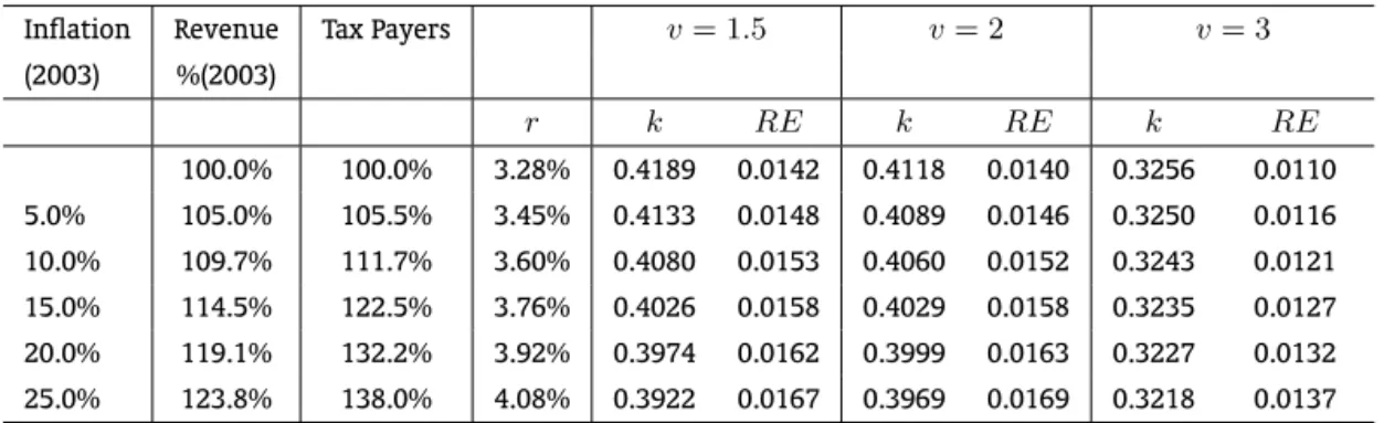
Table 5 presents the size, progressivity and redistributive effect of the income tax for a set of syn-thetic inflation rates (5, 10, 15, 20 and 25 percent) assuming no inflation adjustment. These results reveal that income tax revenue is quite responsive to inflation. If no adjustment is carried out, 10 per-cent inflation would increase the revenue, in real terms with respect to 2003, by 9.7 perper-cent and the tax burden from 3.28 to 3.6 percent. The number of taxpayers is even more responsive to fiscal drag, 10 percent inflation would increase it by 11.7 percent. If no adjustment was applied on the income tax after a 20 percent increase in prices the number of taxpayers would rise by almost a third.
Table 5: Income tax size, progressivity and redistribution: no adjustment to synthetic inflation rates
Inflation Revenue Tax Payers v= 1.5 v= 2 v= 3
(2003) %(2003)
r k RE k RE k RE
100.0% 100.0% 3.28% 0.4189 0.0142 0.4118 0.0140 0.3256 0.0110
5.0% 105.0% 105.5% 3.45% 0.4133 0.0148 0.4089 0.0146 0.3250 0.0116
10.0% 109.7% 111.7% 3.60% 0.4080 0.0153 0.4060 0.0152 0.3243 0.0121
15.0% 114.5% 122.5% 3.76% 0.4026 0.0158 0.4029 0.0158 0.3235 0.0127
20.0% 119.1% 132.2% 3.92% 0.3974 0.0162 0.3999 0.0163 0.3227 0.0132
25.0% 123.8% 138.0% 4.08% 0.3922 0.0167 0.3969 0.0169 0.3218 0.0137
Note: Indices computed through the comparison of income “before” and “after” income tax.ris the size of the tax,kis the Kakwani progressivity index,REis the redistributive effect. For details on indices and on inequality aversion parameterv, see subsection 4.3.
Source: Authors’ own elaboration using BRAHMS, version 2003b.
reducing progressivity at the top. In fact, after 15 percent inflation progressivity would be higher for
v= 2compared tov= 1.5.
Table 6: Proportion of income tax by deciles: no adjustment to synthetic inflation rates Deciles 2003 Inflation
5% 10% 15% 20% 25%
1 0.0% 0.0% 0.0% 0.0% 0.0% 0.0%
2 0.0% 0.0% 0.0% 0.0% 0.0% 0.0%
3 0.0% 0.0% 0.0% 0.0% 0.0% 0.0%
4 0.0% 0.0% 0.0% 0.0% 0.0% 0.0%
5 0.0% 0.0% 0.0% 0.0% 0.0% 0.0%
6 0.0% 0.0% 0.0% 0.0% 0.0% 0.0%
7 0.0% 0.1% 0.1% 0.1% 0.2% 0.2%
8 0.6% 0.7% 0.9% 1.0% 1.2% 1.4%
9 4.5% 5.0% 5.4% 5.9% 6.3% 6.7%
10 94.8% 94.2% 93.6% 93.0% 92.3% 91.7% Total 100.0% 100.0% 100.0% 100.0% 100.0% 100.0%
Note: Deciles are computed for individuals ranked according to household disposable income (HDI) equivalised by the “modified OECD” equivalence scale. HDI are calculated as the sum of all income sources of all household members net of income tax and social insurance contributions.
Source: Authors’ own elaboration using BRAHMS, version 2003b.
On the other hand, redistribution (RE) would rise with fiscal drag. Thus, recalling equation (5), the reduction in progressivity (k) is more than compensated by the higher tax burden (r). The redistributive effect increases monotonically with the inflation rate. Usingv= 2,10percent inflation would increase redistribution by 8.7 percent, while 20 percent inflation would increase it by 17 percent. With regard to the inequality aversion parameterv, in proportional terms, rises in redistribution are higher for larger values ofv. For an inflation of 20 percent, the redistributive effect would rise by 14, 17 and 19 percent withv equal to 1.5, 2 and 3, respectively. Contrary to results presented in Table 4, redistribution is no longer monotonically lower for larger values ofv. For an inflation larger than 15 percent, redis-tribution with v = 2would be higher than withv = 1.5. Nevertheless, as the redistributive effect of the income tax is quite low, even after relatively high levels of inflation, income tax redistribution would still be rather low. If no adjustment was introduced after 25 percent inflation, the reduction on income inequality (measured by the standard Gini coefficient) would be from 0.5241 to 0.5212 and not statistically significant.21
6.2. Income tax, inflation and adjustment in the period 2003-2008
Since 1999 all major changes on the rules of the personal income tax have been eventual increases in monetary parameters.22Although such increases were discontinuous and not in line with the inflation
in any particular year, they consisted on uniform increases of the monetary elements of the income tax (deductions, limits and thresholds) by a single factor. Thus, it is generally accepted that such increases
21Confidence intervals, calculated using bootstrap techniques, are available from authors on request.
22In 1999 the highest rate of personal income tax was raised from 25 to 27.5 percent. Interestingly, the tax schedule limits and
were partial and time-lagged inflation adjustments. This irregular indexation policy has been revised in recent years. It is clear from Table 7 that the uprating factors for 2005 and 2006 were considerably higher than inflation, probably aiming to compensate the lack of adjustment in previous years. A regular and transparent indexation approach has been introduced for the 2007-2010 period. Income tax monetary parameters are uprated by the inflation target set by the Central Bank.
Table 7: Income tax adjustment and inflation: 1997–2010
Year Income tax schedule Inflation
Band 1 (reais) Band 2 (reais) Adjustment (%)
1997 900 1,8 – 5.2
1998 900 1,8 0.0 1.7
1999 900 1,8 0.0 8.9
2000 900 1,8 0.0 6.0
2001 900 1,8 0.0 7.7
2002 1,058 2,115 17.5 12.5
2003 1,058 2,115 0.0 9.3
2004 1,058 2,115 0.0 7.6
2005 1,164 2,326 10.0 5.7
2006 1,257 2,512 8.0 3.1
2007 1,314 2,625 4.5 3.5*
2008 1,373 2,743 4.5 4.1*
2009 1,435 2,867 4.5 –
2010 1,499 2,996 4.5 –
Note: Inflation index: extended consumer price index (Índice Nacional de Preços ao Consumidor Amplo – IPCA).
* Central Bank IPCA forecast.
Source: Banco Central do Brasil (2007).
How recent inflation adjustment policies have affected the burden and distributional effect of the income tax in Brazil? What would have been the burden and distributional effect of the income tax if no inflation adjustment had been applied between 2003 and 2008? In order to answer those questions we run two sets of simulations: actual inflation adjustmentandnoadjustment. In both scenarios all monetary inputs to the income tax are increased in line with the inflation rates in Table 7. However, while in the former scenario all income tax monetary parameters are uprated in line with the adjust-ment factors in Table 7, in the later all income tax rules are held as in 2003. It should be borne in mind that the simulations ofactual inflation adjustmentin 2004-2008 do not take into account the real evolution of incomes and of other determinants of income tax (e.g., household composition or medical and education expenses), therefore the results cannot be interpreted as forecasts of the income tax on those years.
Those indicators fall further in 2007 and 2008 as inflation forecasts are lower than inflation targets for both years. Comparing 2008 and 2003 scenarios, the revenue (in real terms) falls by 2.6 percent, the tax burden to 3.19 percent and the number of taxpayers by 6 percent. In contrast, if no inflation adjustment was applied in the period, the revenue (in real terms) would rise by 25 percent, the tax burden to 4.12 percent and the number of taxpayers by 39 percent.
Table 8: Income tax size, progressivity and redistribution: actual inflation and adjustment
Year Revenue Tax payers v= 1.5 v= 2 v= 3
% (2003)
r k RE k RE k RE
2003 100.0% 100.0% 3.28% 0.4189 0.0142 0.4118 0.0140 0.3256 0.0110
Actual inflation adjustment
2004 107.4% 108.3% 3.53% 0.4105 0.0150 0.4074 0.0149 0.3246 0.0119
2005 103.4% 104.5% 3.39% 0.4151 0.0146 0.4098 0.0144 0.3252 0.0114
2006 98.7% 95.0% 3.24% 0.4204 0.0141 0.4126 0.0138 0.3258 0.0109
2007 97.8% 94.4% 3.21% 0.4214 0.0140 0.4131 0.0137 0.3259 0.0108
2008 97.4% 94.0% 3.19% 0.4218 0.0139 0.4133 0.0136 0.3260 0.0108
No adjustment
2004 107.4% 108.3% 3.53% 0.4105 0.0150 0.4074 0.0149 0.3246 0.0119
2005 113.3% 121.3% 3.72% 0.4040 0.0156 0.4037 0.0156 0.3237 0.0125
2006 116.6% 124.9% 3.84% 0.4002 0.0160 0.4016 0.0160 0.3231 0.0129
2007 120.4% 133.0% 3.96% 0.3959 0.0163 0.3991 0.0165 0.3224 0.0133
2008 125.0% 139.1% 4.12% 0.3908 0.0168 0.3960 0.0170 0.3216 0.0138
Notes: Indices computed through the comparison of income “before” and “after” income tax.ris the size of the tax,kis the Kakwani progressivity index,REis the redistributive effect. For details on indices and on inequality aversion parameterv, see subsection 4.3.
Source: Authors’ own elaboration using BRAHMS, version 2003b.
Consistently with results presented above, progressivity falls/rises and redistribution rises/falls when the level of adjustment is lower/higher than inflation. Proportional changes in progressivity are larger for the inequality aversion parameter v = 1.5, while changes in redistribution are larger forv = 3. Nevertheless, in all cases the changes in progressivity and redistribution are very small. The largest progressivity and redistribution variations are in the year 2004, usingv = 2progressivity decreases by 1.1 percent and redistribution increases by 6.7 percent. As, over the whole (2003-2008) period, the adjustment is larger than inflation, progressivity is slightly larger and redistribution lower 2008 than in 2003. Thus, measured by the standard Gini coefficient (v = 2), income inequality rises from 0.5241 to 0.5244 (this difference is not statistically significant). If no inflation adjustment had been implemented over whole period, progressivity would have fallen to 0.3960 and redistribution would have increased to 0.0170 (usingv = 2). In that case, the standard Gini coefficient would have fallen to 0.52108 (this difference is also not statistically significant).
6.3. The likely effects of inflation on tax payments under behavioural responses
In the standard model of labour supply, a progressive income tax influences individual choices through a change in the marginal wage as well as a change in lump sum income. This can be illus-trated using a two-good diagram, following Auerbach (1985, p.85).23 For example, consider the case of
the Brazilian income tax, with an exemption limit and two marginal rates,t1et2. This leads to three after-tax wages: w0 equal to pre-tax wage;w1 = w0(1−t1)ew2 = w0(1−t2). The individual’s pre-tax and after-tax budget lines are represented in Figure 2.H1andH2correspond to hours supplied at the intersection of the two tax brackets.
The important point to note is that the effect of this progressive tax on the behaviour of an individ-ual whose preferred hours of work were previously betweenH1andH2is equivalent to the effect of a
proportional tax at ratet1plus lump sum incomey1. If the individual’s preferred hours of work were
previously aboveH2the effect of the tax is equivalent to the effect of a proportional tax at ratet2plus
lump sum incomey2.24
By reducing the real value of deductions and the real width of the tax brackets, inflation decreases the lump sum incomes of all individuals above the exemption limit. As long as they remain on the same budget segment, this would induce more labour supply. However, there may be some ‘bracket creep’: some individuals initially below the exemption limit may be moved to the second budget segment, with a positive marginal ratet1and some people previously on the second budget segment may shift
to the third tax bracket, with higher marginal ratet2.
As can be seen from Figure 2, shifting to a higher tax bracket reduces marginal wage and increases lump sum income. The change in wage alone leads to offsetting ‘income and substitution effects’ (just as in the standard economic analysis of price changes), and the change in lump sum income generates a further ‘income effect’ which induces less labour supply. Thus, in the case of individuals which remain on the same tax bracket, including all those in the highest tax bracket, inflation will cause them to increase work effort and therefore pay more tax. But, if an individual is moved to a higher tax bracket, labour supply responses can go either way, depending on preferences. In the case of Brazil, we might expect a positive net effect of inflation on income tax revenue in the presence of labour supply responses, possibly higher than that estimated in this paper, since the bulk of the tax is collected from people in the highest tax bracket.25
It should be noted that in attempting to capture labour supply responses to tax changes, it is crucial to correctly associate individuals with differing wage and income responses to appropriate points on the tax schedule, since wage elasticities and effective marginal tax rates diverge substantially across individuals. As argued by Blundell (1996), it is difficult to believe that such task can be achieved without a micro-simulation (behavioural) model. On the other hand, there are channels through which inflation may alter the behavioural and distributional effects of taxation which can only be captured within a general equilibrium framework. For instance, it is well known that inflation tends to increase the real capital income tax burden in a nominally based tax system and thus reduces the real net return on savings. A number of articles have used general equilibrium growth models to analyse how this affects the real equilibrium and the growth path of the economy, as well as wealth distribution.26
7. CONCLUSIONS
Making use of a tax-benefit microsimulation model for Brazil to simulate different scenarios regard-ing the level of inflation and the adjustment of the income tax rules, we have assessed the potential revenue and distributive effects of inflation on the income tax.
23See also Hausmann (1985). 24Lump sum incomes
y1andy2are also referred to as ‘virtual incomes’.
Our results show that the income tax revenue is quite elastic to fiscal drag. Income tax burden would increase if tax rules are not adjusted for inflation. Nevertheless, as the income tax burden in Brazil is quite low, it would remain rather low if inflation is moderate and the period without adjustment is not excessively long.
The influence of fiscal drag on the distributive properties of the income tax is considerable. Our simulations show that income tax progressivity would decrease if it is not adjusted for inflation. The reduction level would increase with inflation. As the income tax only affects the top of income distribu-tion, progressivity changes would be significantly lower for measures that give larger weight to bottom income groups.
As to redistribution, inflation-induced reductions in progressivity are more than compensated by higher tax burdens. Redistribution increases with inflation if the income tax is left unadjusted. Yet again, as the redistributive effect of the income tax is quite low, even after relatively high levels of inflation, income tax redistribution would still be rather low. If no adjustment was introduced after 25 percent inflation, the reduction on income inequality (measured by the standard Gini coefficient) – from 0.5241 to 0.5212 – would not be statistically significant.
After a period of no or irregular adjustment, income tax has been considerably adjusted for inflation in recent years. In 2005 and 2006, inflation adjustment compensated the lack of adjustment in previous years. From 2007 to 2010, income tax monetary parameters are adjusted in line with the inflation target set by the Central Bank. As the rate of adjustment for 2003-2008 is larger than the expected inflation, the revenue (in real terms), tax burden and the number of taxpayers in 2008 are lower than in 2003. Progressivity is slightly higher, but not enough to compensate the lower tax burden as redistribution goes down.
Hence, our findings contradict the view that adjusting income tax for inflation would reduce the tax base andprogressivity. Quite the opposite, our results show that the lack of adjustment reduces progressivity, although it increases the redistributive effect through a larger tax burden. On the other hand, we agree that the income tax base is small and that most alternative taxes (mainly indirect ones) are potentially less progressive (if not regressive) than the income tax. However, in our view, fiscal drag should not be used as an alternative to tax reform. First, because it only would significantly change the redistributive effect of the income tax if inflation is exceptionally high or no adjustment is carried out for a long period of time. Second, because the size of income tax base, revenue and redistributive effect should be determined by transparent and explicit policy objectives that are consistent over time rather than by circumstantial inflation rates.
Careful modelling of policy alternatives can contribute to the design of the income tax to reach policy objectives. This paper has illustrated the potential of tax-benefit microsimulation techniques in assessing the revenue and distributive effect of tax reforms and of policies under different scenarios (such as different levels of inflation and policy rule adjustment).
BIBLIOGRAPHY
Aronson, J. R., Johnson, P., & Lambert, P. (1994). Redistributive effect and unequal tax treatment. Eco-nomic Journal, 104:262–70.
Atkinson, A. B. (1980). Horizontal equity and the distribution of the tax burden. In Aaron, H. J. & Boskin, M., editors,The Economics of Taxation. Brookings Institution, Washington, D.C.
Auerbach, A. J. (1985). The theory of excess burden and optimal taxation. In Auerbach, A. J. & Feldstein, M., editors,Handbook of Public Economics. North-Holland, Elsevier, Amsterdam.
Blackorby, C. & Donaldson, D. (1978). Measures of relative equality and their meaning in terms of social welfare.Journal of Economic Theory, 18:59–80.
Blundell, R. (1996). Labour supply and taxation. In Devereux, M., editor,The Economics of Tax Policy. Oxford University Press, Oxford.
Bresser-Pereira, L. C. (1991). A lógica perversa da estagnação: Dívida, déficit e inflação no Brasil. Revista Brasileira de Economia, 45:187–211.
Donaldson, D. & Weymark, J. A. (1980). A single parameter generalization of the Gini indices of inequal-ity. Journal of Economic Theory, 22:67–86.
Duclos, J. Y. (2000). Gini indices and the redistribution of income. International Tax and Public Finance, 7:141–162.
Duclos, J. Y. & Araar, A. (2006). Poverty and Equity: Measurement, Policy and Estimation with DAD. Series: Economic Studies in Inequality, Social Exclusion and Well-Being, volume 2. Springer, New York.
Durevall, D. (1999). Inertial inflation, indexation and price stickiness: Evidence from Brazil. Journal of Development Economics, 60:407–421.
Feldstein, M. (1997). The costs and benefits of going from low inflation to price stability. In Romer, C. & Romer, D., editors,Reducing Inflation: Motivation and Strategy. University of Chicago Press, Chicago. Feldstein, M. (1999).The Costs and Benefits of Price Stability. The University of Chicago Press, Chicago. Franco, G. (2004). Auge e declínio do inflacionismo no Brasil. In Giambiagi, F. e. A., editor,Economia
Brasileira Contemporânea, 1945/2004. Editora Campus, Rio de Janeiro.
Goetz, C. J. & Weber, W. F. (1971). Intertemporal changes in real federal income tax rates, 1954-70.
National Tax Journal, 24:51–63.
Hausmann, J. (1985). Taxes and labor supply. In Auerbach, A. & Feldstein, M., editors,Handbook of Public Economics. North-Holland, Amsterdam.
Heer, B. & Sussmuth, B. (2007). Effects of inflation on wealth distribution: Do stock market participation fees and capital income taxation matter? Journal of Economic Dynamics and Control, 31.
Hoffmann, R. (2002). O efeito potencial do imposto de renda na desigualdade. Pesquisa e Planejamento Econômico, 32:107–113.
Immervoll, H. (2005). Falling up the stairs: The effect of bracket creep on household incomes. Review of Income and Wealth, 151:37–62.
Immervoll, H. (2007). Fiscal drag– An automatic stabiliser? In Bargain, O., editor,Micro-Simulation in Ac-tion: Policy Analysis in Europe Using EUROMOD, pages 165–198. Elsevier, Research in Labor Economics. Immervoll, H., Levy, H., Nogueira, J. R., O’Donoghue, C., & Siqueira, R. (2006). Simulating Brazil’s tax-benefit system using BRAHMS, the Brazilian household microsimulation model. Economia Aplicada, 10:203–223.
Jarvis, G. (1977). Real income and average tax rates: An extension for the 1970–75 period.Canadian Tax Journal, 25:206–15.
Kakwani, N. C. (1977). Measurement of tax progressivity: An international comparison. Economic Journal, 87:71–80.
Lugaresi, S. & Nicola, F. D. (1991). Tax policy and income redistribution in Italy. TIDI Discussion Paper n. 152.
Majocchi, A. (1976). Effetti distorsivi dell’inflazione nel quadro dell’imposizione progressiva sul reddito delle persone fisiche. In Gerelli, E., editor,Imposte e Inflazione, pages 110–54. Franco Angeli, Milan. Ministério da Economia (2005). Orçamento social do governo federal 2001-2004. Brasília: Secretaria de
Política Econômica, Ministério da Fazenda.
Ministério do Seguro Social (2005). Anuário estatístico da previdência social. Brasília. Neudeck, W. (1981). Inflation and the taxation of capital income. Empirica, 8.
OECD (2005). Economic survey of Brazil 2005. Paris: Organisation for Economic Co-operation and Development.
OECD (2006). OECD in figures 2006–2007. Paris: Organisation for Economic Co-operation and Develop-ment.
Okun, A. M. (1975). Equality and Efficiency, the Big Tradeoff. Brookings Institution, Washington, D.C. Plotnick, R. D. (1981). A measure of horizontal equity.Review of Economics and Statistics, 63:283–88. Ramalho, V. (2003). Simonsen: Pioneiro da visão inercial da inflação. Revista Brasileira de Economia,
57:223–238.
Redmond, G., Sutherland, H., & Wilson, M. (1998). The Arithmetic of Tax and Social Security Reform: A User’s Guide to Microsimulation Methods and Analysis. Cambridge University Press, Cambridge. Reis, M. & Ulyssea, G. (2005). Cunha fiscal, informalidade e crescimento: Algumas questões e propostas
de política. Texto para Discussão n. 1068, IPEA.
Reynolds, M. & Smolensky, E. (1977). Public Expenditure, Taxes and the Distribution of Income: The United States 1950, 1961, 1970. Academic Press, New York.
Rocha, S. (2002). O impacto distributivo do imposto de renda sobre a desigualdade de renda das famílias.
Pesquisa e Planejamento econômico, 32:73–105.
Secretaria da Receita Federal (2001). Considerações sobre o imposto de renda da pessoa física no Brasil. Texto para Discussão n. 14, Brasília.
Secretaria da Receita Federal (2004). O imposto de renda das pessoas físicas no Brasil. Estudos Tribu-tários 14, Brasília.
Sunley, E. M. J. & Pechman, J. E. (1976). Inflation adjustment for the individual income tax. In Aaron, H. J., editor,Inflation and the Income Tax, pages 153–72. Brookings Institution, Washington.
Taxation Review Committee (1974). Preliminary report. Canberra.
Von Furstenberg, G. M. (1975). Individual income taxation and inflation.National Tax Journal, 27:117–25. Vukelich, G. (1972). The effect of inflation on real tax rates. Canadian Tax Journal, 20:327–42.
Wagstaff, A., Dooslaer, E. V., Burg, H. V. D., Calonge, S., Christiansen, T., Citoni, G., Gerdtham, U. G., Gerfin, M., Gross, L., Hakinnen, U., John, J., Johnson, P., Klavus, J., Lachaud, C., Lauridsen, J., Leu, R. E., Nolan, B., Peran, E., Propper, C., Puffer, F., Rochaix, L., Rodriguez, M., Schellhorn, M., Sundberg, G., & Winkelhake, O. (1999). Redistributive effect, progressivity and differential tax treatment: Personal income taxes in twelve OECD countries. Journal of Public Economics, 72:73–98.
Yitzhaki, S. (1983). On an extension of the Gini index. International Economic Review, 24:617–28. Yitzhaki, S. (1998). More than a dozen alternative ways of spelling Gini.Research on Economic Inequality,