On evaluation of shape sensitivities of non-linear critical loads
E. Parente Jr.
1;∗;†and L. E. Vaz
21Civil Engineering Department;Federal University of Pernambuco;Recife;Brazil
2Civil Engineering Department;Pontical Catholic University of Rio de Janeiro;Rio de Janeiro;Brazil
SUMMARY
The present paper focuses on the evaluation of the shape sensitivities of the limit and bifurcation loads of geometrically non-linear structures. The analytical approach is applied for isoparametric elements, leading to exact results for a given mesh. Since this approach is dicult to apply to other element types, the semi-analytical method has been widely used for shape sensitivity computation. This method combines ease of implementation with computational eciency, but presents severe accuracy problems. Thus, a general procedure to improve the semi-analytical sensitivities of the non-linear critical loads is presented. The numerical examples show that this procedure leads to sensitivities with sucient accuracy for shape optimization applications. Copyright ? 2002 John Wiley & Sons, Ltd.
KEY WORDS: shape sensitivity analysis; structural optimization; non-linear structures; object-oriented programming
1. INTRODUCTION
The structural shape optimization aim is to nd a shape, dened by a set of design variables, that minimizes a cost function and satises a set of constraints. Generally, these constraints are dened in terms of structural responses, such as displacements and stresses. Currently, the shape optimization process is normally performed under the assumption of linear behaviour, which renders the structural optimization simple and ecient. It is important to note that this approach leads to economic and safe designs for a wide variety of structures.
However, there are some practical structures for which the load-carrying capacity can be strongly decreased by non-linear eects. As pointed out in a classic work [1], optimization can generate structures with severe instability problems. However, some recent works [2–4] have been demonstrating that this is not a intrinsic characteristic of the structural optimization,
∗Correspondence to: E. Parente Jr., Civil Engineering Department, Federal University of Pernambuco, Av.
Academico Helio Ramos s/n, CEP 50740-530, Recife, Pernambuco, Brazil
†E-mail: [email protected]
Contract=grant sponsor: CNPq-Brazilian Council for Scientic and Technological Development
but rather a problem associated with the use of inadequate analysis procedures and the lack of appropriate optimization constraints.
It is well known that the gradient-based algorithms are the most ecient for structural optimization. To nd a search direction for the optimization process, these algorithms require the evaluation of the derivatives of the objective and constraint functions with respect to the design variables. Therefore, errors in the evaluation of these gradients lead to severe convergence problems and, possibly, to the failure of the optimization process. It should be noted that these gradients depend on the derivatives (sensitivities) of structural response quantities.
In order to generate safe designs it is necessary to consider the geometrically non-linear eects and include critical load constraints, in addition to the traditional displacement and stress constraints, in the optimization problem. Thus, it is necessary to compute the sensitivities of these structural responses. Since the procedures to the computation of the displacement and stress sensitivities are already well known, this paper focus on the computation of the sensitivities of the non-linear critical loads.
It is important to note that there are several works about the computation of the sensitiv-ities of critical loads of non-linear structures. However, most of them deal only with limit points [5–11]. There are also works dealing with bifurcation points, but some of them do not specically address nite element applications [12, 13], while others are restricted to the semi-analytical approach [2, 3]. Therefore, the aim of this paper is to discuss dierent approaches for the computation of the shape sensitivities of limit and bifurcation loads of non-linear structures discretized in nite elements.
Initially, the expressions for FE geometrically non-linear analysis are presented with em-phasis on isoparametric continuum elements formulated using the total Lagrangian approach. After that, the basic expressions required for the analytical evaluation of the sensitivities of limit and bifurcation loads are derived using the same matrix notation used for geometrically non-linear analysis. The sensitivity of vectors and matrices of the continuum isoparametric elements are detailed discussed. Whenever possible, the original expressions are modied in order to achieve more computational eciency.
The analytical approach produces exact sensitivities for a given nite element mesh, increas-ing the eciency and the reliability of the shape optimization process. However, it should be noted that the application of the analytical approach to more complex elements is not simple, and alternative procedures should be addressed. Therefore, the present work also discusses the nite dierence and the semi-analytical approaches. The latter combines the eciency of the analytical approach with the generality and simplicity of the nite dierence approach. However, since the semi-analytical sensitivities can present severe accuracy problems, this approach is not reliable.
In order to obtain a computational procedure for the evaluation of the critical load sensitivity of non-linear structures that maintains the positive aspects of the semi-analytical approach, but does not present its accuracy problems, the rened semi-analytical approach [8, 9, 11] will be extended in the present work to deal with non-linear bifurcation loads.
in the comparison of the quality of the sensitivities computed by the semi-analytical and the rened semi-analytical methods.
2. GEOMETRICALLY NON-LINEAR ANALYSIS
The linear analysis is based on the hypothesis that the displacements and strains developed in the structure due to the applied loads are innitesimal. Thus, the geometry of the structure remains constant during the loading process and there is no practical dierence between the original and the deformed congurations. Therefore, the equilibrium equations can be written in the undeformed (known) geometry.
However, there are some slender structures which can present large displacements without the development of large strains and with the stresses not growing beyond the elastic limit of the material. Moreover, there are other structures which present bifurcation buckling, due to compressive membrane stresses, even when the displacements are small (classic elastic instability problem). In both cases, the linear analysis cannot predict correctly the load carrying capacity of the structure. Therefore, it is necessary to use the non-linear equilibrium equations to describe the structural behaviour.
There are dierent procedures for geometrically non-linear analysis. In the total Lagrangian (TL) approach, all static and kinematic variables at the current state are referred to the initial conguration, while in the updated Lagrangian (UL) approach they are referred to the last calculated conguration. Therefore, dierent stress and strain tensors should be used for each formulation, but, if appropriate stress–strain relationships are used, both procedures lead to the same results [14].
The total and the updated Lagrangian approaches are based on the use of sophisticated stress and strain tensors in order to deal with the eects of nite rigid body rotations. On the other hand, the corotational approach solves this problem providing a single frame that continuously rotates with the element. The use of this rotating reference system eliminates the rigid body rotations prior to strain computation, allowing the application of the standard small strain–displacement relationship [15].
In the comparison of the non-linear formulations it is important to remember that, in a shape optimization standpoint, the structural responses are functions of the element undeformed geometry, which is dened by a set of design variables. Thus, the aim of the shape sensitivity analysis is to compute the changes in the structural responses caused by changes in the initial geometry. An important dierence between the non-linear formulations is that the integrations necessary to compute the vectors and matrices of the nite elements formulated according to the TL and the corotational approaches are carried out over the initial geometry, while the integrations of the UL elements are carried out over a deformed geometry. Therefore, the element vectors and matrices are explicit functions of the initial geometry for the former approaches and implicit functions for the latter.
corotational approach is applied mainly for the development of beam and shell elements. As the application of the analytical method for these elements is not straightforward, their formulation will not be discussed in the present paper.
2.1. Basic equations
Whether the displacements are large or small, the equilibrium conditions between the internal and external forces must the satised. Using the Principle of Virtual Work, the equilibrium equations of a FE model can be written as
r(u; ) =g(u)−f=0 (1)
where u is the nodal displacement vector, r is the unbalanced load vector, g is the internal force vector, f is reference load vector, and is the load factor. The element internal force vector is given by
g(u) =
V
BtAdV (2)
where V is the element volume, A is the stress vector and B comes from the strain vector (U) variation
U=@U
@uu= B(u)u (3)
For small strains, but large displacements and rotations, a linear stress–strain relationship can be assumed. Thus, one can write
A=CU (4)
where C is the elastic constitutive matrix.
In order to evaluate the nodal displacements, it is necessary to solve the system of non-linear equilibrium equations using an iterative method. However, it is important to note that to determine the behaviour of a given structure it is not sucient to compute a single equilibrium point, but to trace the equilibrium path of this structure. The simplest procedure to trace the equilibrium path is the Load Control Method with Newton–Raphson iterations. This method is based on the linearization of the equilibrium equations at a prescribed load level.
For a xed load factor, the linearization of Equation (1) yields
Ku= −r (5)
where the tangent stiness matrix is dened by
Ku=@g
@uu=
V Bt@A
@udV+
V
@Bt
@uAdV
u (6)
After the computation of the incrementsu, the new displacement vectorun is computed from the old vector uo using the well-known expression
0
B
A C
λ
u
(a)
L2 B
L1
0 u
λ
(b)
Figure 1. Equilibrium paths and critical points.
and the internal force vector is computed based on this updated vector. The iterations are performed until the residual is smaller than a prescribed tolerance. In order to trace the equilibrium path, it is necessary to increment the load factor and repeat the iteration cycle. It should be noted that the stiness matrix and the internal force vector are assembled from element contributions exactly as is carried out in linear problems.
The Load Control Method can trace the load–displacement curve before the occurrence of a limit point (segment OA in Figure 1(a)), but generally it will fail to converge beyond this point. Moreover, even if it converges it will miss the segment ABC, leading to erroneous conclusions about the structural behaviour. To trace the complete equilibrium path depicted in Figure 1(a), it is necessary to use more sophisticated path-following methods, as the Dis-placement Control Method [16], the various forms of the Arc Length Method [17–19] or the Generalized Displacement Control Method [20], to cite some examples.
2.2. Critical points
The analysis of a given structure is not complete without the determination of its load carrying capacity. Thus, it is necessary to compute the critical points of the load–displacement curve. There are two dierent types of critical points, as depicted in Figure 1(b). A limit point arises when the equilibrium path reaches a local extremum, as the points L1 (maximum) and L2 (minimum), while a bifurcation occurs when dierent equilibrium paths meet at a certain point, as the point B in Figure 1(b).
A point (u, ) of the load–displacement curve is a critical point when the stiness matrix of the FE model is singular. Thus, a critical point can be detected using the condition
det K(u; ) = 0 (8)
An alternative approach to the critical point detection is to use the null eigenvector condition
K(u; )v=0 (9)
point. To perform this task, it is convenient to describe the load–displacement curve using a single parameter (s) that never decreases during the loading process, like the curve length.
Using the parametric form, Equation (1) can be written as
r(u(s); (s)) =0 (10)
and its dierentiation w.r.t. the curve parameter yields
dr ds=
@r
@u du ds +
@r
@
d
ds=K
du ds −f
d
ds=0 (11)
Using condition (9) and the symmetry of the stiness matrix, it can be shown that vtK=0 at a critical point. Therefore, the multiplication of Equation (11) by vt leads to the condition
(vtf)d
ds= 0 (12)
which can be used to classify the critical points. As pointed out early, a limit point is char-acterized by the fact that the load–displacement curve reaches an extremum value, so the condition d=ds= 0 must hold for these points. Therefore, the following criteria can be used to classify the critical points:
vtf = 0 ⇒ limit point
vtf= 0 ⇒ bifurcation point (13)
It is interesting to note that the bifurcation points are characterized by the orthogonality between the external load vector and the buckling mode.
From a computational standpoint, it is not convenient to use expression (13) since the scalar product vtf does not precisely vanishes. Thus, a slightly modied criteria will be used in this work:
|cos(v;f)|¿tol ⇒ limit point
|cos(v;f)|6tol ⇒ bifurcation point (14)
where the cosine of the angle between the vectors v andf is computed from
cos(v;f) = v tf
v f (15)
and tol is a tolerance in the range between 10−5 and 10−7. It is important to note that the criteria adopted in the present work is not aected by the number of degrees of freedom of the FE model.
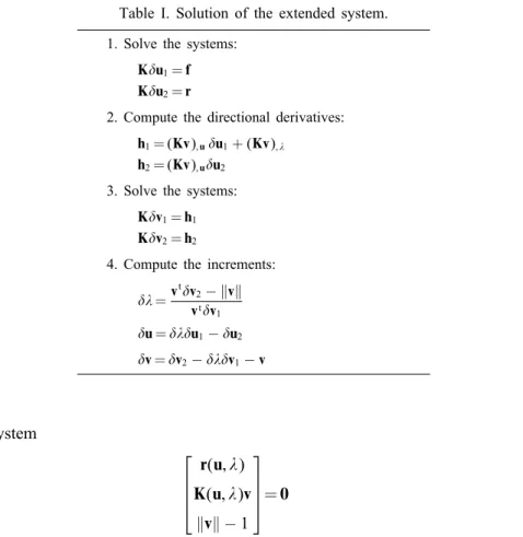
Table I. Solution of the extended system.
1. Solve the systems:
Ku1=f Ku2=r
2. Compute the directional derivatives:
h1= (Kv);uu1+ (Kv); h2= (Kv);uu2
3. Solve the systems:
Kv1=h1 Kv2=h2
4. Compute the increments:
=v
t
v2− v vtv
1
u=u1−u2
v=v2−v1−v
extended system
r(u; ) K(u; )v
v −1
=0 (16)
where the eigenvector length constraint is necessary to avoid the trivial solution (v=0) [21]. The solution of this extended system gives the critical point (u, ) as well as the buckling mode (v), which can be used for the critical point classication. Since only one eigenvector is included in the system, this procedure is restricted to limit and simple bifurcation points [21].
The linearization of expression (16) yields the system
K 0 −f
(Kv);u K (Kv);
0t vvt 0
u
v
= −
r
Kv
v −1
(17)
which allows the computation of the increments u, v and . This system has 2n+ 1 variables and equations, but it can be solved in a simple and ecient manner using an appropriate scheme, as shown in Table I.
due to the extra backsubstitutions and the computation of the vectors h1 and h2 becomes less important when the number of dofs increases and the computational cost is dominated by the factorization process.
A central step for the success of the computation of critical points using extended systems is the computation of the vectors h1 and h2. These vectors depend on the derivatives (Kv);u and (Kv); , but it is known that for displacement independent loads (Kv); =0. Starting from the expression of the strain energy, it is possible to nd the analytical expressions of the directional derivatives [21]. However, the practical application of the analytical approach is limited to simple elements, and to nd a more general solution, it is interesting to use an approximate method.
Considering the symmetry of the stiness matrix, the application of the nite dierence method [22] yields
h1= 1
[K(u+v)u1−K(u)u1] =
1
[K(u+v)u1−f]
h2= 1
[K(u+v)u2−K(u)u2] =
1
[K(u+v)u2−r]
(18)
which can be used to compute h1 and h2 in a simple and ecient way. Moreover, since they do not depend on the element type, these expressions can be implemented once and used for all available element types of a given FE program. Generally, a perturbation () in the range (10−3¡v=u¡10−8) leads to accurate results [2]. Finally, it is important to note that the computation of the global vectors h1 and h2 is carried out summing up the contribution of each element, using exactly the same procedure applied for the assembly of the global internal force vector.
2.3. Isoparametric elements
In order to present the basic features of the isoparametric elements based on the TL formu-lation, the plane stress case will be used as an example. However, the extension to plane strain, axisymmetric and three-dimensional cases is straightforward [14, 15]. In the isopara-metric formulation, the displacement eld inside each element is interpolated from the nodal displacements
u v
=
Niui
Nivi
=Niui=
N1 0 · · · Nm 0 0 N1 · · · 0 Nm
u1
v1 .. .
um
vm
=Nu (19)
where the shape functions (Ni) are polynomials that depend on the element parametric co-ordinates (r, s) and m is the number of element nodes. In this equation and in the rest of this paper, the summation convention for repeated indices is used. The equation above shows that the interpolation matrix N for a generic element can be written as
To allow the use of elements with curved sides, the element geometry is interpolated from the nodal co-ordinates (xi, yi) using the same functions used to the displacement interpolation. Thus,
x=Nixi and y=Niyi (21) The TL formulation is based on the use of the Green–Lagrange strains and of the second Piola–Kirchho stresses. For the plane stress case, the strains are
x y xy =
u; x
v; y
u; y+v; x + 1 2(u
2 ; x+v2; x) 1
2(u 2 ; y+v2; y)
u; xu; y+v; xv; y
(22)
Therefore, the Green–Lagrange strains are computed from the displacements derivatives. Using Equation (19), it can be shown that these derivatives can be computed from
u; x
u; y
v; x
v; y = l11 l12 l21 l22 =
Ni; xui
Ni; yui
Ni; xvi
Ni; yvi =
Ni; x 0
Ni; y 0 0 Ni; x 0 Ni; y
ui vi
=Giui=Gu (23)
where Ni; x and Ni; y are the derivatives of the shape functions w.r.t. the Cartesian co-ordinates
x and y, respectively. It should be emphasized that, using the TL approach, these derivatives are computed over the undeformed geometry.
Using Equations (22) and (23), the Green–Lagrange strains inside an element can be com-puted from
U=B(u)u (24)
where the matrix B, which relates the element strains with the nodal displacements, is given by the sum of two matrices
B=B0+ 12BL(u) (25)
The matrix B0 is the same matrix used in linear analysis and BL is a matrix which depends linearly on the nodal displacements. The matricesB0 and BL have the same format of matrix N, but each sub-matrix is given by
B0i=
Ni; x 0 0 Ni; y
Ni; y Ni; x (26) and
BLi=
l11Ni; x l21Ni; x
l12Ni; y l22Ni; y
l11Ni; y+l12Ni; x l21Ni; y+l22Ni; x
Performing the variation of the strain vector, as in Equation (3), it can be shown [15, 24] that matrix B is given by
B=B0+BL(u) (28)
Using Equation (6) it can be shown [15, 24] that the stiness matrix is composed by two terms, the elastic stiness matrix and the geometric (or initial stress) stiness matrix
K=KE+KG=
V
BtCB dV+
V
GtSGdV (29)
where the stress matrix is given by
S=
x xy 0 0
xy y 0 0
0 0 x xy
0 0 xy y
(30)
The stresses that appear in this matrix correspond to the total strains and should be computed using Equation (4). It can be realized that the geometric matrix (KG) is symmetric since the stress matrix (S) is symmetric. On the other hand, the elastic stiness matrix (KE) is symmetric whenever the constitutive matrix (C) is symmetric. Thus, the tangent stiness matrix of the isoparametric elements based on the TL formulation is generally symmetric.
The derivativesNi; x andNi; y used in the previous expressions can be computed from
Ni; x
Ni; y
=
r; x s; x
r; y s; y
Ni; r
Ni; s
=
Ni; r
Ni; s
(31)
where is the inverse of the Jacobian matrix
J=
Ni; rxi Ni; ryi
Ni; sxi Ni; syi
(32)
Finally, the element innitesimal volume which appears in Equations (2) and (29) can be written as
dV=t|J|d =t|J|drds (33)
where t is the element thickness. Owing to the use of the TL formulation, the Jacobian matrix and its determinant are computed using the co-ordinates (xi, yi) of the undeformed geometry. The integrations necessary to compute the internal force vector and the stiness matrix generally are carried out using the Gauss quadrature.
It is interesting to note that the expressions presented in this section to the computation of
The generality of the isoparametric formulation can be fully exploited using the concepts of the object-oriented programming. Applying this paradigm, the FEMOOP program [25] de-nes the behaviour of a generic nite element in the cElement base class, while the derived class (cElcParam) denes the behaviour of the isoparametric elements using generic methods to compute U, A, g, and K.
Moreover, an object of cElement class contains pointers to two auxiliary classes. The
cAnmModel class is responsible for the specic features of the type of analysis being per-formed (e.g. truss, plane stress, plate, shell, solid, etc.), while the cShapeclass deals with the geometric and eld interpolation aspects of an element (e.g. Q4, Q8, T6, BRICK8, BRICK20, TET10, etc.).
Therefore, the implementation of the geometric non-linear capability in this program was rather simple, since only two modications were necessary. The rst was the derivation of a sub-class (cElcParamTL) to implement the dierences between the generic behaviour of linear and non-linear isoparametric elements, and the second was the implementation of methods to compute the matrices BL, G, and S for the dierent analysis models. It should be emphasized that modications in the cShape class were not necessary.
3. SENSITIVITY ANALYSIS
The dierent methods for the computation of the sensitivity of the critical load factor w.r.t. shape variables will be discussed in following sections. The aim is to present the complete expressions required for sensitivity computation and to compare the methods considering the aspects of accuracy, eciency and computer implementation.
It is important to note that there are two basic approaches to sensitivity computation. The discrete approach is based on the dierentiation, numerical or analytical, of the governing equations of the FE model. On the other hand, the continuum approach [26, 27] is based on the dierentiation of the variational equations of the problem before the FE discretization. Due to its simplicity, only the discrete approach is used in the present work.
3.1. Analytical method (AM)
This section presents the mathematical expressions required for the analytical computation of the shape sensitivities of the critical points of non-linear structures. In order to simplify the presentation, and without loss of generality, it will be considered a structure described by only one design variable (x). Initially, the general expressions required for sensitivity computation will be presented. These expressions are independent of the element type and valid for shape and size variables. After that, these general equations will be specialized for shape variables and isoparametric elements.
The system of equilibrium equations of a FE model can be written as
g(u; x)−f(x) =0 (34)
where u and are implicit functions of the design variable x. The dierentiation of this equation yields
@g
@u du dx+
@g
@x −
d
dxf−
df
Since K=@g=@u, this expression can be rewritten as
Kdu dx −
d
dxf=
df dx −
@g
@x=p (36)
where p is known as the ‘pseudo-load’ vector. It is important to note that the pseudo-load computation involves only the partial derivative of the internal force vector w.r.t. the design variablex. Therefore, the displacements are kept xed during the computation of the pseudo-load vector.
Considering a xed load level, the term d=dx vanishes. Thus, the sensitivity of the nodal displacements can be computed from
Kdu
dx=p (37)
These sensitivities are necessary to deal with displacement and stress constraints, which are applied at a load level smaller than the critical one.
On the other hand, multiplying Equation (36) by vt and using the critical load condition (vtK=0), the expression
d
dx= −
vtp
vtf (38)
which can be used for the computation of the critical load sensitivity, is obtained. The com-putation of the critical load sensitivity using this expression is simple and ecient, once the buckling mode (v) was already evaluated during the determination of the critical point. How-ever, it is important to note that, according to condition (13), the product vtf vanishes in bifurcation points. Thus, Equation (38) can be used only for limit points.
The sensitivity computation for bifurcation loads is more complex, and it is necessary to consider two dierent situations. In the regular case, a change in the variable x modies the critical load, but preserves the bifurcation. On the other hand, in the singular case, a change in the variable x eliminates the bifurcation, and a limit point arises. In the present work, only the regular case will be considered.
The computation of the sensitivity of a bifurcation load requires the consideration of the critical point condition
K(u; x)v(x) =0 (39)
The dierentiation of this equation w.r.t. x yields d(Kv)
dx = @(Kv)
@u du dx+
@K
@xv+K @v
@x=0 (40)
which depends on the sensitivity of the nodal displacements (du=dx). Using Equation (36), this sensitivity can be written as
du dx=
d
dxuf +up (41)
where the vectors uf and up can be computed from Kuf =f Kup=p
while the substitution of (41) in (40) leads to
d
dx @(Kv)
@u uf +
@(Kv)
@u up+
@K
@x v+K @v
@x=0 (43)
Finally, multiplying this equation by vt and using the condition vtK=0, the expression
d
dx= −
vt(h p+w) vth
f
(44)
which can be used for computation of the sensitivity of critical loads, is obtained. To produce a more compact format, this sensitivity was written using the auxiliary vector
w=@K
@x v (45)
and the directional derivatives
hf= (Kv);uuf hp= (Kv);uup
(46)
It can be noted that these directional derivatives can be computed using an expression similar to Equation (18).
Theoretically, it will be impossible to use expression (44) to sensitivity computation, since the calculation ofuf andup requires the factorization of the stiness matrix at a point where this matrix is singular. In order to avoid this problem, some works [2, 27] suggest to compute the sensitivities at a point close to the critical point. However, numerical experiments show that the extended systems will precisely reach a singular point only for very simple structures. Thus, expression (44) can be applied for practical problems.
It is important to note that Equation (44) is valid for limit and bifurcation points. However, since it requires the computation of the sensitivity of the stiness matrix as well as the evaluation of the directional derivatives hf and hp, its computational cost is far superior to the cost of expression (38). Thus, expression (44) should be used only for bifurcation points. A more ecient procedure for the computation of sensitivity of bifurcation loads can be derived using the adjoint approach [12, 27]. This technique denes a scalar equation including the equilibrium and the critical point conditions
vtKv−\t(g−f) = 0 (47)
where \ is the vector of the Lagrange multipliers used to enforce the equilibrium. The dif-ferentiation of this equation leads to
dvt dxKv+v
t
@(Kv)
@u du dx +
@(Kv)
@x
−\t
Kdu
dx −
d
dxf−p
= 0 (48)
but using the condition Kv=0 and grouping some terms, it is possible to write
(vt(Kv);
u−\tK) du dx+v
t
@K
@x v+K @v
@x
+\t
d
dxf+p
It can be realized that it is possible to avoid the computation of the sensitivity of the nodal displacements (du=dx) forcing the coecient of this term to be null. When the stiness matrix is symmetric, this can be accomplished computing \ through the solution of the system
K\= (Kv);uv=hv (50)
where the directional derivative hv can be computed using a expression similar to (18). It is important to note that the vector \ is independent of the design variable x. Thus, even for problems with several variables, the vector \ needs to be computed only once.
Finally, using the condition vtK=0 and the denition of w given by Equation (45), it is possible to write the expression
d
dx= −
vtw+\tp
\tf (51)
which allows the computation of the sensitivity of the critical loads. This equation is more ecient than Equation (44), since it does not require the computation of the vectors uf,up, hf andhp. Moreover, this advantage increases with the number of design variables. However, the multiplication of Equation (50) by vt leads to the condition vt(Kv);
uv= 0. Since this condition holds only for symmetric bifurcations, the use of Equation (51) is not consistent for asymmetric bifurcations [12].
3.2. Shape variables
Expressions (38), (44), and (51) form the basis for the computer implementation of the evalu-ation of the sensitivity of the non-linear critical loads w.r.t. shape and size variables. However, some additional considerations are necessary to deal with shape variables eciently. Using geometric modelling concepts [28–30], the geometry of a given structure can be described through its boundary curves (or surfaces). Therefore, the shape of the structure is determined by the geometry of its boundary curves, and the parameters that control the shape of these curves are the design variables.
On the other hand, the geometry of a FE mesh is described only by the nodal co-ordinates. Using the chain rule, the critical load sensitivity w.r.t. the design variablex can be written as
d
dx= @ @aj
daj
dx (j= 1: : : ns) (52)
where ns is the number of nodes linked to the design variable x, and aj denotes the x, y or z co-ordinate of a given node. It is important to note that the shape variables are directly associated only to the boundary nodes (active elements) of the FE mesh. Thus, the number of active nodes (ns) generally is much smaller than the total number of nodes. This is the case of the beam depicted in Figure 2, where only the marked nodes are active for a change in the beam length.
In order to use expression (52), it is necessary to compute the critical point sensitivity w.r.t the nodal co-ordinates, which can be performed using expression (44). This procedure requires the computation of one directional derivative and one backsubstitution for each co-ordinate
Figure 2. Active nodes and elements.
design variable x
p=df
dx− @g
@x= @f
@aj daj
dx − @g
@aj daj
dx =
@f @aj
− @g
@aj
da
j dx =paj
daj
dx (53)
and evaluating the sensitivity of the critical load using Equation (44). It should be noted that this procedure requires a w vector given by
w=@K
@xv=
@K
@aj daj
dx
v=
@K
@aj v
da
j dx =waj
daj
dx (54)
Since the number of design variables is smaller than the number of active nodes (ns), this approach is more ecient than the former one. The vectors paj and waj of the structure are
assembled summing up the element contributions, exactly as is carried out for the internal force vector. However, an element will contribute to these global vectors only whenaj refers to a node connected to this element.
3.3. Isoparametric elements
This section presents the expressions for the sensitivity computation of the internal force vector (g) and of the stiness matrix (K). The sensitivity of the reference load vector (f) is computed using the same expressions applied in linear analysis, and will not be discussed here. The internal force vector of a plane stress element based on the TL formulation is given by
g=
BtAt|J|d (55)
Thus, the sensitivity of this vector w.r.t. aj can be computed from
g′=
V
( B′tA|J|+ BtA′|J|+ BtA|J|′)td (56)
In this expression and in the rest of this paper, f′ denotes @f=@aj. In order to minimize the number of products between matrices and vectors, this expression can be rewritten as
g′=
( B′tA+ BtA∗)|J|d (57)
where the vector A∗ is dened as
A∗=A′+ A
|J||J|
It is important to note that, due to the TL formulation,|J| is computed using the undeformed geometry (initial co-ordinates) of the structure, and |J|′ represents the change of the initial volume due to changes in the shape variables.
The partial dierentiation of Equation (4) w.r.t. the co-ordinate aj yields
A′=CB′u (59)
where
B′=B′0+1 2B
′
L (60)
It should be noted that in the dierentiation of expression (4) the displacements are kept xed, as is required in the computation of the pseudo-load vector. Therefore, Equation (59) cannot be used for computation of stress sensitivity.
Dierentiating Equation (28), the sensitivity of B matrix can written as
B′=B′0+B′L (61)
where the dierentiation of Equation (26) w.r.t. aj yields
B′0i=
N′ i; x 0
0 N′ i; y
Ni; y′ Ni; x
(62)
The matrix BL is more complex, but dierentiating Equation (27), this sensitivity can be written as
B′Li=BIL′i+BIIL′i (63)
where
BI′
Li=
l11Ni; x′ l21Ni; x′
l12Ni; y′ l22Ni; y′
l11Ni; y′ +l12Ni; x′ l21Ni; y′ +l22Ni; x′ (64) and
BIIL′i=
l′11Ni; x l′21Ni; x
l′12Ni; y l′22Ni; y
l′
11Ni; y+l′12Ni; x l′21Ni; y+l′22Ni; x
(65)
Finally, the dierentiation of Equation (23), yields
l′11
l′12
l′ 21 l′ 22 =
Ni; x′ 0
Ni; y′ 0 0 N′ i; x
0 N′ i; y
As shown by equations above, the computation of the sensitivities of the matrices B, B, and G depends on the sensitivities of Ni; x and Ni; y w.r.t. aj. The computation of these sensi-tivities involves the dierentiation of the matrix , which is not explicitly known. However, dierentiating the expression J=I, the sensitivity of can be written as
′= −J′= − (67)
SinceNi; r andNi; s do not depend on the nodal co-ordinates, the dierentiation of the Jacobian matrix (32) w.r.t aj leads to
J′=
Nk; r 0
Nk; s 0
(68)
when aj corresponds to the x co-ordinate of the element node of index k (aj=xk). Thus, using (68), the matrix can be written as
=
Nk; x 0
Nk;y 0
(69)
It should be noted that the sensitivities for aj=yk are easily obtained permuting the columns of the matrix. Finally, using (31) and (67), the sensitivities ofNi; x andNi; y can be computed from
Ni; x′ Ni; y′
=′
Ni; r
Ni; s
= −
Ni; r
Ni; s
= −
Ni; x
Ni; y
(70)
To complete the evaluation of the sensitivity of the internal force vector, it is necessary to compute the sensitivity of |J|. Using the chain rule, this sensitivity can be written as
|J|′=@|J|
@Jkl
Jkl′ (71)
where Jkl are the components of the Jacobian matrix. On the other hand, using the expression which gives the inverse of a matrix as a function of its cofactors [31], it can be shown that
@|J|
@Jkl
= lk|J| (72)
Therefore, the sensitivity of |J| w.r.t. aj is given by
|J|′= lkJkl′|J|= trace(J′)|J|= trace()|J| (73)
Finally, according to Equations (69) and (73), this sensitivity can be computed from
|J|′=Nk; x|J| (74)
while the sensitivity for aj=yk can be obtained permuting Nk; x by Nk;y.
is necessary to compute the sensitivity of the stiness matrix in order to evaluate the critical load sensitivity. The elastic stiness matrix of a plane stress element is given by
KE=
BtCBt|J|d (75)
Since the elastic constitutive matrix does not depend on the element nodal co-ordinates, the sensitivity of K w.r.t. aj can be written as
K′E=
( B′tCB|J|+ BtCB′|J|+ BtCB|J|′)td (76)
where the matrices that appear in this expression were already presented. Rearranging some terms, the sensitivity of the elastic stiness matrix can be written as
K′E=
( B′tCB + BtCB∗)t|J|d (77)
where
B∗= B′+ |J| ′
|J| B (78)
It should be noted that expression (77) is more ecient than (76) since the number of matrix products was minimized.
The geometric stiness matrix of a plane stress element is given by
KG=
GtSGt|J|d (79)
and the dierentiation of this expression w.r.t. aj yields
K′G=
(G′tSG|J|+GtS′tG|J|+GtSG′+GtSG|J|′)td (80)
Dening the auxiliary matrix G∗ as
G∗=G′+ |J| ′
|J|G (81)
the sensitivity of the geometric stiness matrix can be written as
K′G=
(G′tSG+GtS′tG+GtSG∗)t|J|d (82)
which is a more ecient form than (80), since the number of matrix products was minimized. The sensitivities that appear in this expression were already presented, except the sensitivity of the stress matrix. Dierentiating Equation (30) w.r.t. aj, this sensitivity can be written as
S′=
′x ′xy 0 0
′xy y′ 0 0 0 0 ′x ′xy
0 0 ′xy y′
(83)
Using the auxiliary matrices B∗ andG∗, the number of triple products of matrices necessary to the computation of the sensitivity of the stiness matrix was reduced. However, according to Equations (44) and (51), the sensitivity of the critical load does not require the sensitivity of the stiness matrix, but only the computation of the w vector. Using Equation (45), the w vector of a given nite element can be written as
w=K′v=K′Ev+K′Gv=wE+wG (84)
where
wE=
( B′tCBv + BtCB∗v)t|J|d (85)
and
wG=
(G′tSGv+GtS′tGv+GtSG∗
v)t|J|d (86)
Therefore,w can be evaluated using only products of matrices by vectors, without computing triple product of matrices, which are much more computationally expensive.
3.4. Finite dierence method (FDM)
This is the simplest method to compute the derivative of a generic function (f). The basic idea is to approximate the derivative using the expression
df
dx ≈
f(x+ x)−f(x)
x (87)
where x is the perturbation size. Generally, the perturbation size is computed from a given relative perturbation (), through the expression
x=x (88)
The accuracy of the FDM is strongly dependent on the perturbation size. It is well known that very small values lead to rounding errors, due to the computer representation of real numbers, while large perturbations lead to truncation errors, once expression (87) is exact only in the limit (x→0). However, a relative perturbation between 10−5 and 10−8 generally leads to results with sucient accuracy for engineering applications.
The FDM is very simple to code, since Equation (87) does not require any specic knowl-edge about the computation of the function f. Therefore, its implementation is completely independent of the nite elements used in the numerical discretization, which allows the use of the analysis program as a ‘black box’, leading to the possibility of utilization of commercial softwares whose source code is not known.
3.5. Semi-analytical method (SAM)
The aim of this method is to combine the simplicity and the generality of the FDM with the eciency of the AM. To accomplish this task, the SAM uses the general expressions of the AM for the sensitivity of displacements and critical loads, but computes the sensitivities of f, g, and K by nite dierences.
The resulting method is much more ecient than the FDM, since it is not necessary to perform new structural analyses. Moreover, its implementation is much more simple than the implementation of the AM, once the expressions used for sensitivity computation are independent of the element formulation, and the dierent elements can be handled by the same computational procedure. This characteristic is very important, since the application of the AM to non-linear elements more complex than the continuum isoparametric elements discussed in this paper is cumbersome and error prone.
The accuracy of the SAM is controlled by the size of the perturbation used in the numerical dierentiation. Using the same perturbation range recommended for the FDM, the results obtained by the semi-analytical approach are satisfactory for a great number of practical structures. The combination of eciency, simplicity, and accuracy, led to the wide application of this method in structural optimization problems.
However, there are some problems involving shape variables where the SAM presents severe accuracy problems. As these problems do not occur in the FDM, it can be concluded that these errors are caused by the numerical dierentiation of the internal force vector and of the stiness matrix, which are inherent to the semi-analytical approach [31]. This problem does not occur in the dierentiation of the external load vector.
The accuracy problems of the SAM are more serious for elements having simultaneously translations and rotations as degrees of freedom, like beam, plate, and shell elements. It was detected that, for these elements, the sensitivity errors increase with the mesh renement [32, 33]. The accuracy problems also occur for elements having only translations, like truss and continuum isoparametric elements, but in this case the errors do not depend on the mesh renement [34]. The initial studies about the accuracy problems of the SAM are carried out for linear structures, and it was veried that these abnormal errors occur for structures whose displacement are dominated by rigid body rotations [31]. Since slender structures can present large rigid rotations, the accuracy problems also occur in geometrically non-linear analysis.
Dierent procedures have been proposed to eliminate the abnormal errors presented by semi-analytical sensitivities. The most simple is to use second order accurate central dierences in substitution to the rst-order accurate standard forward dierences. This solution preserves the simplicity of the semi-analytical approach, but increases the computational cost of sensitivity evaluation since it requires two function evaluations for each variable, while the forward dierences require only one new function evaluation per variable. Moreover, the accuracy problem is alleviated, but not solved.
3.6. Rened semi-analytical method (RSAM)
Another procedure to elimination of the abnormal errors presented by the semi-analytical sensitivities is the Rened Semi-Analytical Method. This method is based on the use of orthogonality relations between the element internal forces and the rigid body motions in order to improve the quality of the semi-analytical sensitivities. It does not lead to exact results, since the truncations errors are inherent to the numerical dierentiation, but it has been able to eliminate the abnormal errors occurring in structures whose displacement eld is dominated by rigid body rotations. Thus, the results produced by this method are suciently accurate for use in shape optimization.
This method has been successfully applied in the sensitivity computation of linear structures [36, 37], of linearized buckling problems [38], as well as of geometrically non-linear structures [8, 9, 11], including the sensitivity of limit points. In the present work, this method will be extended in order to deal with non-linear bifurcation points.
According to Equation (36), the pseudo-load vector is computed using the sensitivity of the internal force vector and the sensitivity of the external load vector. However, it is well known that the nite dierence computation of the sensitivity of the external load vector leads to accurate results. Thus, the errors in the pseudo-load vector are due to the numerical dierentiation of the internal force vector, and the rst aim of the RSAM is to improve the sensitivity of this vector.
Independent of the particular formulation of a given nite element, the internal force vec-tor must satisfy the free body equilibrium conditions. From elementary mechanics, three-dimensional problems have three equations expressing the equilibrium of forces
Fx= 0 Fy= 0 Fz= 0 (89)
and three equations expressing the equilibrium of moments
Mx= 0 My= 0 Mz= 0 (90)
It should be noted that for plane problems there are only two equations for forces and one for moments. The equilibrium conditions of a given nite element can be written as
g·rk= 0 (91)
where rk is a auxiliary vector obtained from (89) and (90). Since the work done by a system of forces in equilibrium (as g) through a rigid body displacement is null, it can be realized that the vectors rk represent the element rigid body motions.
The RSAM use condition (91) to improve the semi-analytical sensitivity of the internal force vector. To this aim, it can be realized that the vectorsrk form a basis of a vector space, and, to be used eectively, these vectors should be mutually orthogonal (ri·rj= 0, for i=j), but not unitary. The dierentiation of Equation (91) w.r.t aj yields
g′·rk+g·r′k= 0 (92)
As discussed previously, the pseudo-load vector is given by
p=f′−g′ (93)
Decomposing the vector g′ in a component in the vector space spanned byr
k and in another component orthogonal to this space, the expression above can be rewritten as
g′=g ′·r
k rk·rkrk−
g′−g
′·r k rk·rkrk
(94)
while the substitution of (94) in (93), leads to the expression
p=f′−g′+g ′·r
k rk·rk
rk− g′·r
k rk·rk
rk (95)
On the other hand, Equation (92) implies that
g′·rk= −g·r′k (96)
Moreover, it will be shown later that the vectors r′k can be computed analytically without diculty. Therefore, this equation shows that the projection of g′ over rk can be computed in an exact manner even when g′ is computed by nite dierences.
Finally, using Equation (96), the pseudo-load vector can be computed from
p=f′−g′+ g ′·rk
rk·rk rk+
g′·rk rk·rk
rk (97)
However, in the computational implementation, it is more ecient to use the expression
p=f′−g′+krk; k=
g′·rk+g·r′k rk·rk
(98)
From the equations above, it can be noted that the objective of the present method is to replace the components ofg′ in the direction of rk, which are inaccurately evaluated by nite dierences, by its analytical derivative, which can be easily computed. It can be shown that the RSA method corrects the sensitivity of the internal force vector in such way that condition (92) is exactly satised even when g′ is computed by nite dierences [11].
The computation of the pseudo-load vector is sucient for displacement and limit load sen-sitivities. However, to deal with bifurcation points, it is necessary to compute the sensitivity of the stiness matrix, and a condition similar to (91) is required. This condition can be obtained from the dierentiation of Equation (91) w.r.t. the nodal displacements, which leads to
Krk+Rkg=0; where Rk=
@rk
@u (99)
The equilibrium of linear structures is written in the undeformed conguration. Thus, the vectors rk are independent of the nodal displacements, and Rk=0 for linear structures.
The dierentiation of Equation (99) w.r.t. the co-ordinate aj yields the condition
This condition is satised by the analytical sensitivities, but when the semi-analytical approach is applied, it was veried in this work that this condition holds only for the equations associ-ated with the equilibrium of forces. Using the above equation, the following expression can be written as
K′rk= −(Kr′k+Rkg′+R′kg) (101)
The eigenvector v can be decomposed in a component in the vector space spanned by the rigid body modes (v1) and in another one orthogonal to this space (v2). Thus,
v=v1+v2=krk+ (v−krk); k= v·rk
rk·rk (102)
The substitution of this equation in the expression of the w yields
w=K′v=K′v1+K′v2=kK′rk+K′v−kK′rk (103)
Finally, using Equation (101), the above expression can be rewritten as
w=K′v−kK′rk−kKr′k−kRkg′−kR′kg=K′v−z (104) where
z=k(K′rk+Kr′k+Rkg′+R′kg) =kzk (105)
It should be realized that the vector z represents a correction to the vector w. Obviously, this correction vanishes when the sensitivity of the stiness matrix is computed by the analyti-cal method. On the other hand, for semi-analytianalyti-cal sensitivities, the Equation (100) is satised only for the translation modes (equilibrium of forces). Thus, for structures whose eigenvec-tor is dominated by rigid body rotations, the errors can be critical, and the semi-analytical sensitivities will lead to very inaccurate results. However, the numerical examples presented in this paper will show that the correction given by the vector z can reduce dramatically the errors caused by the numerical dierentiation of the stiness matrix of these structures.
Equation (104) is interesting since the conventional w and the correction term appear sep-arately. However, from a computational standpoint, it is more ecient to compute w using the expression
w=K′v2−Kv1′ −kRkg′−kR′kg; where v′1=kr′k (106)
since the number of matrix-vector products is minimized.
It is important to note that expressions (98) and (106) are completely independent of the formulation of a given element and can be implemented in a generic form. Moreover, the vectors rk and r′k, as well as the matrices Rk and R′k, depend only on the element degrees of freedom, and can be easily computed in an exact manner, as will be discussed in the next sections.
3.6.1. Non-orthogonal basis vectors. The computation of the rened sensitivities requires the computation of the orthogonal basis vectors (rk) and the corresponding sensitivities (r′
The number and nature of the vectors rk depend on the nite element degrees of free-dom, but do not depend on the particular formulation of the element. Thus, a generic three-dimensional element will be used here to illustrate the proposed procedure. These elements have three degrees of freedom per node, and all degrees of freedom are translations. There-fore, the internal force vector is composed only by forces. The same occurs for truss, plane stress, plane strain, and axisymmetric elements. On the other hand, for structural elements, as beam and plate, the internal force is composed by forces and moments, but the procedure for determination of the vectors rk is the same.
The rst three basis vectors represent the equilibrium of forces in the global directions (x,
y, z), and can be written as
r1
r2
r3
= [F1 F2 · · · Fn] (107)
where n is the number of element nodes and each sub-matrix Fi is given by
Fi=
1 0 0
0 1 0
0 0 1
(108)
These vectors do not depend on the nodal co-ordinates. Thus, the sensitivity of these vectors w.r.t. aj is simply given by
r′k=0; for k63 (109)
The remaining vectors represent the equilibrium of moments around the three global axis (x; y; z), and can be written as
r4
r5
r6
= [M1 M2 · · · Mn] (110)
Since the equilibrium should be written in the deformed conguration, each sub-matrix Mi is given by
Mi=
0 −(zi+wi) (yi+vi) (zi+wi) 0 −(xi+ui)
−(yi+vi) (xi+ui) 0
(111)
where (xi; yi; zi) are the element nodal co-ordinates and (ui; vi; wi) are the nodal displacements. Dierentiating this equation w.r.t. aj, it can be shown that
M′i=
0 0 0
0 0 −1
0 1 0
and
Mi′= 0; for j=i (113)
It should be noted that the sensitivities for aj=yi andaj=zi are obtained in a similar manner and will not be discussed here.
To deal with bifurcation points, it is necessary to compute the matrices Rk and R′k for the given nite element. Using the indicial notation, the matrix Rk can be written as
Rkij=
@rkj
@ui
(114)
Thus, the dierentiation of translation modes, which are given by Equation (108), yields
Rk=0; for k63 (115)
since these modes do not depend on the nodal displacements. On the other hand, the case of the rotation modes are not so simple, and the application of Equation (114) to the vectors given in expression (111) leads to
Rk=
Ak1 0 · · · 0
0 Ak2 · · · 0
..
. ... . .. ...
0 0 · · · Akn
for 46k66 (116)
where each sub-matrix Ak
i is given by
A4i =
0 0 0
0 0 1
0 −1 0
; A5i=
0 0 −1
0 0 0
1 0 0
; Ai6=
0 1 0
−1 0 0
0 0 0
(117)
Since the matrices Rk do not depend on the nodal co-ordinates, their dierentiation w.r.t. aj yields
R′k=0; for k= 1; : : : ;6 (118)
3.6.2. Orthogonalization procedure. Using the Gram–Schmidt orthogonalization procedure [39], the orthogonal basis vectors rk can be computed from
rk= rk− k−1
p=1
apkrp; where apk = rk·rp rp·rp
(119)
Since the rst three vectors rk are already mutually orthogonal, the application of this proce-dure leads to
rk= rk; for k63 (120)
The dierentiation of Equation (119) w.r.t. aj allows to compute the vectors r′k from
r′k= r′k−
k−1
p=1
(apk′rp+apkr ′
p) (121)
To compute these sensitivities in an exact manner, it is necessary to evaluate the terms apk′. However, according to Equation (98), the vectors r′
k are used only to compute the scalar product g·r′
k, which is given by
g·rk′=g·r′k−
k−1
p= 1
(apk′g·rp+apkg·r ′
p) (122)
On the other hand, using the equilibrium condition (g·rp= 0), the Equation (122) can be rewritten as
g·r′k=g·r′k−k−1 p= 1
apkg·r′p=g·
r′k−k−1
p= 1
apkrp′
(123)
The equation above implies that, in thecomputer implementationof the RSAM, the vectors r′
k can be simply computed using the equation
r′k= r′k−k −1
p= 1
apkr′p (124)
Therefore, it is not necessary to compute the terms apk′. Moreover, according to Equations (120) and (109), it can be realized that
r′k=0; for k63 (125)
Thus, the orthogonalization procedure only needs to be applied to the vectors associated with the equilibrium of moments. Since the vectors associated with the equilibrium of forces are independent of the nodal co-ordinates and mutually orthogonal, Equations (120) and (125) are valid for dierent element types.
To deal with bifurcation points, it is necessary to compute the matrices Rk and R′k. According to Equation (99), each Rk matrix is given by
Rk=
@rk
@u (126)
Thus, the dierentiation of Equation (119) w.r.t. the nodal displacements yields
Rk= Rk− k−1
p= 1
@ap
k
@u rp+a p kRp
; Rk=
@rk
@u (127)
However, it is important to note that, according to expression (99), the matrices Rk are used only to compute the product Rkg. Therefore, the rst term between the parenthesis does not have to be considered, becauseg·rp= 0. Thus, in thecomputer implementation of the RSAM, the matrices Rk can be computed from
Rk= Rk− k−1
p= 1
The dierentiation of this equation w.r.t. the co-ordinate aj yields
R′k= R′k−
k−1
p= 1
(apk′Rp+apkR ′
p) (129)
Once again, to compute the matrices R′
k in an exact manner, it is necessary to evaluate the terms apk′.
According to Equation (105), the matrices R′
k are used only to evaluate the correction vectors (zk), which, using Equations (124) and (129), can be written as
zk=K′rk+Kr′k− k−1
p=1
(apk′Krp+apkKr ′
p) + Rkg′+ R ′ kg−
k−1
p= 1
(apk′Rpg+apkR ′
pg) (130)
However, according to Equation (99), it is known that Krp+Rpg=0. Thus, the terms asso-ciated with the coecients apk′ vanish, and the vectors zk can simply be written as
zk=K′rk+K
r′k−k
−1
p= 1
apkrp′
+Rkg′+
R′k−k
−1
p= 1
apkR′p
g (131)
This equation shows that, in the computer implementationof the RSAM for evaluation of the bifurcation load sensitivity, the vectors r′
k also can be computed using Equation (124), while the matrices R′
k can be computed from
R′k= R′k−
k−1
p= 1
apkR′p (132)
and the evaluation of the terms apk′ are never required.
As pointed out early, the number of basis vectors depend on the element type, while the dimension of these vectors depend on the number of element nodes. It can be noted that the structure of expression (119) is identical to (124). Therefore, the vectors rk and r′k can be handled using exactly the same computational procedure. Moreover, it is important to note that the orthogonalization procedure is independent of the element type and can be implemented in a generic form.
Examining Equations (128) and (132), it can be realized that the matrices Rk and R ′ k can be handled by a computational procedure similar to the one used to deal with the vectors rk and r′k. Moreover, the careful inspection of these expressions shows that the coecients apk
can be computed only once and used in the calculation ofrk,r′k,Rk, andR′k. Finally, it can be realized that the computation of these vectors and matrices can be carried out simultaneously, increasing the eciency of the sensitivity computation.
3.7. Computer implementation
out the Design Sensitivity Analysis. This base class is responsible for the implementation of the general expressions for sensitivity evaluation presented in Sections 3.1 and 3.2.
On the other hand, the computation of the vectors p and w is dierent for each of the presented methods, and three dierent sub-classes (cAM, cSAM, cRSAM) were created to perform this task. In addition to the creation of these classes, the implementation of the methods for sensitivity computation also required some new implementations in thecElement
and cAnModel classes.
The implementation of the Semi-Analytical Method was the easiest one, because the same expressions to evaluate the vectors p and w are used for all element types. Therefore, these vectors are evaluated by a method implemented in the cElement base class, and none imple-mentation in the derived classes was required.
On the other hand, the Analytical Method is totally dependent on the element formulation and was implemented only for truss and isoparametric elements. To deal with the isoparametric elements, the generic expressions presented in Section 3.3 were implemented in thecElcParam
class, while the methods to compute the matrices B′
L, G′, and S′ for the dierent analysis models were implemented in the sub-classes derived from cAnModel class.
The implementation of the shape sensitivity analysis for non-linear structures did not require new implementations in thecShapeclass, since the methods to compute the sensitivities Ni; x′,
N′
i; y, Ni; z′ , and |J|′ were also used in the sensitivity computation of linear structures, which was previously implemented.
Since the basic expressions of the Rened Analytical Method for the computation of the vectors pandw (Section 3.6), as well as the orthogonalization procedure described in Section 3.6.2, do not depend on the element type, these tasks are performed for appropriate methods implemented in thecElementbase class, which are used for the dierent elements implemented in the program. On the other hand, the vectors rk and r′k, as well as the matrices Rk and R
′ k, do not depend on the element formulation, but depend on the element degrees of freedom. Thus, they are evaluated for specic methods dened for each cAnModel sub-class.
4. NUMERICAL EXAMPLES
This section presents some numerical examples, in order to validate the expressions developed in the previous sections, as well as to compare the results obtained using the dierent methods. The validation of the computer implementation of Analytical Method was performed using results computed by FDM or using reference values found in the literature. It is important to note that, since the three structures analysed here present symmetric bifurcations, expressions (44) and (51) lead to the same results.
The results obtained by the semi-analytical (SA) method for shape sensitivity analysis are compared with the results obtained by the rened semi-analytical method (RSA). To this aim, the relative error (e) for each sensitivity (d) is dened as
e=
d−dAM
dAM
(133)
2 3
4
5 6
7 9
10 8
11
12
13
Pi
h2 h1 z
x
25
18.3 25 18.3
1
Figure 3. Star-shaped truss (EA= 10976:0 kN, h1= 6:25 m, h2= 8:125 m, P= 1:0 kN).
When the AM results are not available, the SA and RSA sensitivities are compared with some reference results found in the literature (dref). To this aim, the sensitivity ratio (r) is dened as
r= d
dref
(134)
Therefore, a unity value indicates the perfect agreement. It should be noted that, dierently of the relative error dened previously, the sensitivity ratio is a signed function. Thus, a negative value implies that the sign of the approximate sensitivity is incorrect, which generally leads to a failure of the optimization process.
To perform the comparison between the SA and the RSA sensitivities, the relative error and the sensitivity ratio are shown as a function of the relative perturbation (). This perturbation is dened as
=s
s (135)
where s is the element projection in the perturbation direction, for plane and solid elements, or the element length, for truss and frame elements.
4.1. Star-shaped truss
This example deals with the hexagonal star-shaped dome depicted in Figure 3, where the design variable is the heighth2. The structure is loaded withP2=P3=P4=P5=P6=P7= 2P1 and all displacements of nodes 8; : : : ;13 are restrained. The behaviour of this structure is highly non-linear, presenting several critical (limit and bifurcations) points. However, the present paper focus only on the rst critical (bifurcation) point.
The truss was modelled using total Lagrangian elements [10, 15], and the bifurcation load computed in this work (cr= 4:540325) agrees with the value found in the literature [40]. The bifurcation load sensitivity evaluated using the Analytical Method was ′
-12.0 -10.0 -8.0 -6.0 -4.0 -2.0 0.0 log(η)
-7.0 -5.0 -3.0 -1.0 1.0
log (e)
SAM RSAM
Figure 4. Relative errors for the star-shaped truss.
Figure 4 shows the errors of the SA and the RSA sensitivities. It is important to note that the displacement eld of this structure is not dominated by large rigid body rotations, then the errors of the SAM are not so large.
However, the gure shows that, for relative perturbations greater than 10−6, the errors of the RSA sensitivities are approximately 100 times smaller than the errors in the SA sensitivities, which represents a signicant improvement given by the proposed method. It is interesting to note that, in the adopted scale, the relative errors of both methods decrease almost linearly with the relative perturbation up to the point where the round-o errors become dominant. Finally, for perturbations smaller than 10−7, the round-o errors are dominant and both methods give approximately the same results.
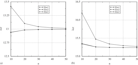
4.2. Circular arch
This example deals with a simply supported circular arch, whose geometry and loading are depicted in Figure 5. The design variable considered in this work is the radius R. The cross-section of the arch is rectangular (b=h= 1:0 m), and the material properties areE= 105MPa and = 0. This structure presents two critical points, where the rst is a bifurcation point and the second is a limit point. The structural behaviour is strongly non-linear, with the development of large displacements and rotations prior to the rst critical point.
According to the literature, the critical points of this structure can be computed from
cr=
EI
PR2 (136)
P
R
L L
Figure 5. Circular arch (R= 100:0 m,L= 80:0 m, P= 833:3333 kN).
10 20 30 40 50
n 12.5
12.75 13 13.25
13.5
λ
cr
Elm1 Elm2 Elm3
10 20 30 40 50
n 15.0
15.5 16.0 16.5
λ
cr
Elm1 Elm2 Elm3
(b) (a)
Figure 6. Critical loads for the circular arch: (a) bifurcation point; and (b) limit point.
In the present work, the circular arch was modeled using dierent plane frame elements formulated using the corotational approach [15]. These elements are initially straight and do not consider the inuence of the shear strains. The simplest formulation (Elm1) computes the axial strain using only the initial and nal straight lengths, while the second formulation (Elm2) enhances this strain adding some shallow arch terms, and the last formulation (Elm3) computes the axial strain based on the condition of constant curvature. It is important to note that these elements have the same degrees of freedom (two translations and one rotation per node). Therefore, the computation of the vectors rk and r′k and of the matrices Rk and R
′ k can be implemented only once and used for the three elements.