Seminonparametric competing risks analysis of recidivism

(www.interscience.wiley.com) DOI: 10.1002/jae.960

SEMI-NONPARAMETRIC COMPETING RISKS ANALYSIS OF

RECIDIVISM

HERMAN J. BIERENSa_{* AND JOSE R. CARVALHO}b

a_{Department of Economics, Pennsylvania State University, University Park, Pennsylvania, USA} b_{CAEN, Universidade Federal do Cear´a, Fortaleza, Brazil}

SUMMARY

In this paper we specify a semi-nonparametric competing risks (SNP-CR) model of recidivism, for misdemeanors and felonies. The model is a bivariate mixed proportional hazard model with Weibull baseline hazards and common unobserved heterogeneity. The distribution of the latter is modeled semi-nonparametrically, using orthonormal Legendre polynomials on the unit interval, and integrated out to make the two durations dependent, conditional on the covariates. The SNP-CR model involved corresponds to a Logit model for felony arrest; hence the validity of the SNP-CR model can be tested by testing the validity of the implied Logit model. The latter will be done by using the integrated conditional moment (ICM) test. In the first instance we have estimated and tested two versions of the SNP-CR model, without and with fixed state effects. However, the ICM test rejects these models. Therefore, we have estimated and tested the model for each state separately. These state models are not rejected by the ICM test. Indeed, the estimation results vary substantially per state. Copyright_{2007 John Wiley & Sons, Ltd.}

Received 3 February 2003; Revised 31 May 2006

1. INTRODUCTION

In 1998, according to a press release from the Department of Justice, the recidivism rate in the United States showed great variation. Where the state of Montana showed the lowest rate of 11%, Utah reported the highest rate of 67%. Within those two extremes, for example, New York appeared with 43.8%, Florida recorded 18.8% and Illinois closed that year with 39.9%. Although these figures are difficult to compare, because of different criteria used to measure recidivism, this variation in recidivism rates is an important issue, especially for those concerned with the justice system. It appears to be a crucial issue for this study as well.

Recidivism, as observed by Maltz (1984), can be understood as a sequence of failures: failure of the correction system in ‘correcting’ the ex-inmate, failure of the ex-inmate in being able to live in a society and failure of the society in completely reintegrating the ex-inmate into a law-abiding environment. Besides the important psychological, sociological and criminological impacts related to recidivism, there are also economic effects; for instance, the forgone labor market earnings, the costs of keeping inmates in prison and jails, and the obsolescence of the inmate’s human capital because of incarceration. It is not surprising that economists, and specifically econometricians, have turned their attention to issues related to recidivism.

Any attempt to make recidivism an operational concept must pay attention to the fact that recidivism is an interval time between two events: a release event and a failure event. The

Ł_{Correspondence to: Herman J. Bierens, Department of Economics, Pennsylvania State University, 608 Kern Graduate}

release event could be from incarceration, from parole supervision, from a halfway house or any other type of official custody. So, the choice of the first event is dependent on the objectives of the study, and to a lesser extent on data availability. The second event deserves more discussion, though. Actually, a great part of the controversy in defining recidivism rests upon it. The modern tendency in criminology has shown that there are three possible definitions for recidivism: rearrest, reconviction and reincarceration1_{. It seems that rearrest has been proven to}

be the most reliable among the three possible measures, as reported in Beck and Shipley (1989) and Maltz (1984). Also Blumstein and Cohen (1979) used rearrest as their measure of recidivism. In this study we will therefore use the time between release from prison and the first rearrest after release as the measure of recidivism, regardless of whether or not a conviction followed the arrest. Besides, our data set does not contain sufficient information about reconviction or reincarceration.

From an econometric perspective, the process of recidivism is best approached by the use of survival models. That was the route followed by Schmidt and Witte (1988). They estimated a set of models of recidivism using state data from the North Carolina Department of Cor-rections. They concluded by noting that the proportional model performed better both in terms of fit as well as prediction than other models used by criminologists, sociologists and statisti-cians.

The use of survival models to study criminal recidivism dates back to the end of the 1970s. The pioneering works of Partanen (1969), Carr-Hill and Carr-Hill (1972), and Stollmack and Harris (1974) are representative of the early literature. Two decades later, a host of important questions have been addressed related to the use of survival models. These include prediction, evaluation of programs and estimation of the effects of regressors on failure times. A good example is Barton and Turnbull (1981), who evaluated a program impact on the process of recidivism, controlling for explanatory variables. Also, Schmidt and Witte (1989) is a relevant application that includes not only regressors but also a ‘split’ parameter representing the probability that recidivism will not occur. The split model can be generalized to include the effect of regressors in the splitting parameter as in Schmidt and Witte (1989). They assumed a Logit model for the split probability.

There is a reasonable appeal to the use of split models in studies of recidivism. Contrary to a model of machine failure, where a component will eventually fail, or in a study of cancer survival, where the patient will eventually die, the assumption that all released prisoners will eventually commit another crime seems inappropriate. Indeed, such an assumption denies any effect of prison treatment on ex-inmates. Another point in favor of split models is made clear in Schmidt and Witte (1989): different regressors affect both the split probability and the time of failure in different ways, and this is important for policy purposes.

Despite the considerations made about split models, its successful use is largely dependent on the availability of data sets with very long follow-up periods. Even with quite long periods in the range of 70– 81 months, as is the case in Schmidt and Witte (1989), the fit presents some difficulties. Only with much longer follow-up periods, such as the 21 years in Escarela et al. (2000), the split model seems feasible.

In their survey of survival analysis applied to recidivism, Chung et al. (1991) made a point about the potential of using competing risks models for explaining recidivism. At that time, they argued that few papers had explored this approach. The few exceptions are Rhodes

1_{These are just broad categories, and admit finer classifications. For a more detailed discussion, see Maltz (1984).}

(1986) and Visher and Linster (1990). Rhodes (1986) consider competing risks, but the appli-cation is to alternative reasons for removal from probation. Visher and Linster (1990) use a bivariate proportional hazard model for misdemeanor and felony recidivism, but they assume that the two durations are independent conditional on the covariates. Some recent exam-ples of this still growing literature are Copas and Heydari (1997) and Escarela et al. (2000). Except for the latter paper, these papers consider recidivism and/or other durations such as the time between reconviction and sentencing (Copas and Heydari, 1997). Escarela et al. (2000) consider three types of crimes: sex offenses, nonsexual violent crimes, and other offenses. They specify exponential distributions for these recidivism durations, conditional on covari-ates, and link then together as a mixture distribution with multinomial Logit probabilities as weights.

There is also a substantial body of literature on structural modeling of criminal behavior. See, for example, Imai and Krishna (2004) and the references therein. The advantage of the structural approach is that it allows for policy experiments, although at the expense of strong behavioral assumptions. Our paper is in the reduced form tradition, but in various aspects different from the literature involved.

First, we use the Bureau of Justice Statistics (BJS) data set, which aims to be a nationally representative data set about recidivism.2Moreover, we consider two different categories of crime: a misdemeanor or a felony. Alone this is not a novelty; Escarelaet al. (2000) consider three types of crimes but they use a different fully parametric model. The actual novelty is the way we model the two recidivism durations involved. Apart from the unobserved heterogeneity distribution, the survival models of the two categories of recidivism are fully specified as mixed proportional hazard models with Weibull baseline hazards. However, we cannot include split probabilities, because in the BJS data set the follow-up period, about 60 months, is too short for that.

The methodological novelties in this paper are twofold. The first one is that the common unobserved heterogeneity is modeled semi-nonparametrically (SNP), using orthonormal Legendre polynomials on the unit interval, similar to the approach in Bierens (2006c), and then integrated out in order to make the two durations dependent conditional on covariates. The second novelty is the finding that the competing risks model involved corresponds to a Logit model for felony arrest; hence the validity of the competing risks model can be tested by testing the validity of the implied Logit model. The latter will be done consistently, using the integrated conditional moment (ICM) test of Bierens (1982, 1990) and Bierens and Ploberger (1997).

In the next section we will discuss the BJS data set. In Section 3 we discuss the semi-nonparametric competing risks (SNP-CR) model. This discussion includes the role of common unobserved heterogeneity in making the durations dependent conditional on covariates, identifica-tion issues, the semi-nonparametric specificaidentifica-tion of the unobserved heterogeneity distribuidentifica-tion, the link between the SNP-CR model and a particular Logit model for felony arrest, and the way to test the validity of this Logit model using the ICM test of Bierens (1982, 1990) and Bierens and Ploberger (1997). Section 4 contains the estimation results. In the first instance we have included state dummy variables in the model to capture the heterogeneity of recidivism rates across states, as mentioned above. However, the ICM test rejects this model. Therefore, we also estimate and test the models for each state separately. These state models are not rejected by the ICM test. It appears that the model parameters vary substantially across states. Finally, in Section 5 we summarize our results and methodological contributions to the literature.

2. THE BUREAU OF JUSTICE STATISTICS DATA ON RECIDIVISM

The data set used in our analysis comes from the Inter-University Consortium for Political and Social Research, henceforth ICPSR, and was originally collected by the Bureau of Justice Statistics (BJS). This data collection represents a major effort by the US Department of Justice to systematically improve the measurement of recidivism. The complexity of the data gathering, its coverage and reach, makes it unique amongst other available data sources on recidivism.

After noticing that one major deficiency in information about the behavior of persons leaving prison was the lack of nationwide data, the BJS initiated a program to overcome this problem. So, in 1983, the Bureaustarted a new National Corrections Reporting Program (NCRP), which follows a convict from admission to prison up to either unconditional release or successful completion of a conditional release or parole. Also, guided by another deficiency, say, the lack of data for states as well as FBI data for each individual, the BJS implemented in 1985 a study to assess the viability of linking state and federal correctional data. Hence, by May, 1987, initial results were published by the BJS, and by the winter of 1989 the ICPSR made the data set available to the public (see ICPSR, 1989).

The BJS data set contains records of 16,355 prisoners from whom both state and FBI rap sheets were found, out of a total population of 108,580 exinmates. The data set is a stratified sample of released prisoners from 11 states who survived up to the follow-up period. Only released prisoners with sentences of at least one year were included. Administrative releases, prisoners who were absent without leave, escapees, releases on appeal, transfers, and those who died in prison, were excluded. So, contrary to other studies that understated recidivism, the data set contains criminal behavior information at both the state and federal level. This represents an improvement in terms of national representativeness, since past studies were restricted to single states or cities. The total number of records is 299,897, and there is information on numerous factors that affect recidivism. Our point of departure to choose a set of regressors of recidivism is Schmidt and Witte (1988). However, we also pay close attention to the criminology literature on recidivism, for instance, Gendreauet al. (1996). The regressors used in Schmidt and Witte (1988) are age at release, time served before the sample sentence, gender, education, marital status, race, drug use, supervision status, participation in programs, and dummies that characterize the type of recidivism. Also, and more importantly from a econometric point of view, we exclude some variables from even initial consideration because of a potential high correlation with other already included variables. This appears to be the case of variables such as past criminal history and sentence length, given the clear movement in the state’s sentencing structure to tie past behavior to length of sentence.

We have selected the covariates shown in Table I. The rescaling of AGE and SENT is done for numerical reasons. Also, we will use dummy variables for the states represented in the BJS sample: California, Florida, Illinois, Michigan, Minnesota, New Jersey, New York, North Carolina, Ohio, Oregon, and Texas. There were a few other covariates available in the sample, in particular education indicators,3 _{but they contained too many missing values to be usable.}

These covariates will be used to explain the dependent variables shown in Table II. Again, the rescaling ofTis done for numerical reasons. The dummy variable Cindicates right-censoring. If

CD1, the durationTcorresponds to the timeTbetween release from prison and the follow-up date April 16, 1988. Since the release dates vary slightly per ex-inmate, so does T. The classification

3_{These education indicators were included in a previous version of this paper, which reduced the effective sample size}

by about 45%. In particular, in California, Ohio and Oregon no information about education is available.

Table I. Covariates MALE Gender indicator

BLACK Race indicator

RELEASE _D0 if released on parole or probation,_D1 otherwise AGE Age, in days/1000

SENT Actual time served, in days/1000, before release

Table II. Dependent variables T_Dmin⊲T1, T2⊳,in days/1000, where

T1Dtime between release and rearrest for a misdemeanor, T2Dtime between release and rearrest for a felony

C_D1 if not rearrested before the follow-up date April 16, 1988

D0 if rearrested before the follow-up date April 16, 1988 FD1 if rearrested for a felony

D0 if rearrested for a misdemeanor

of the type of rearrest, F, is based on the assessment of the arresting officers rather than of a judge or jury. Therefore, a suspected felony arrest may lead to a misdemeanor conviction, or even acquittal. Moreover, in some cases after a misdemeanor arrest the authorities may find out that the ex-inmate was guilty of a felony,4 _{but we do not have information about this.}

The BJS data set is not a random sample. From each but one of the 11 participating states a separate, a representative sample of male and female prisoners was drawn. The exception is Minnesota, where all prisoners were selected. Then, within each group, prisoners were grouped into 24 strata that were defined based on race, age, and type of past offense.5 Finally, an i.i.d. sample was selected within each stratum. Therefore, at first sight the BJS data set seems to be a standard stratified sample (in the terminology of Wooldridge, 2002).

In the BJS data set, however, no ex-inmate in California was released on parole or probation, and in North Carolina and Texas no ex-inmate was rearrested for a felony! Therefore, the representativeness of the stratification is questionable.

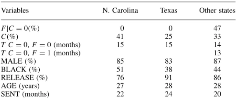
It is known that certain types of sample stratification can render estimators inconsistent and/or inefficient. According to Wooldridge (2001), the stratification issue can be ignored if the strata are constructed entirely based on exogenous variables. However, it seems that in North Carolina and Texas the strata were (directly or indirectly) selected on the basis of the dependent variable F, because it is inconceivable that felony recidivism is absent in these states. Moreover, the sample averages of the variables in Table III do not reveal substantial differences between North Carolina, Texas and the other nine states, except for the absence of felony rearrests in North Carolina and Texas.

On the other hand, it is possible that the absence of felony rearrests in North Carolina and Texas is due to incomplete record keeping, or that potential felons have left these states without a trace.

4_{This was suggested by a referee.}

5_{The offense for which incarceration ended somewhere in 1983. After release, the prisoner belongs to the population}

Table III. Sample averages

Variables N. Carolina Texas Other states

FjCD0⊲%⊳ 0 0 47

C⊲%⊳ 41 25 33

T_jC_D0,F_D0 (months) 15 15 14

T_jC_D0,F_D1 (months) 13

MALE (%) 85 83 87

BLACK (%) 51 38 44

RELEASE (%) 76 91 86

AGE (years) 27 28 28

SENT (months) 22 24 20

3. SEMI-NONPARAMETRIC COMPETING RISKS MODELS

3.1. Bivariate Mixed Proportional Hazard Models

Consider two durations, T1 and T2. Conditional on a vector X of covariates, and a common

unobserved (heterogeneity) variable V, which is assumed to be independent ofX, the durations

T1 andT2 are assumed to be independent:

P[T1 t1, T2 t2jX, V]DP[T1 t1jX, V]P[T2 t2jX, V]

This is a common assumption in bivariate survival analysis (see Van den Berg, 2000). Next, let

Fi⊲tjX, V⊳DP[TitjX, V]D1exp⊲Vexp⊲ˇi0X⊳i⊲t⊳⊳ ⊲1⊳

Si⊲tjX, V⊳D1Fi⊲tjX, V⊳Dexp⊲Vexp⊲ˇ0iX⊳i⊲t⊳⊳ ⊲2⊳

i_D1,2, where 1⊲t⊳D

t

01⊲⊳d and 2⊲t⊳D

t

02⊲⊳d are the integrated baseline hazards

depending on parameter vectors˛1and˛2, respectively. For notational convenience the dependence

of1⊲t1⊳and2⊲t2⊳on parameters is suppressed. Moreover, let

fi⊲tjX, V⊳D∂Fi⊲tjX, V⊳/∂t

DVexp⊲Vexp⊲ˇ0_iX⊳i⊲t⊳⊳exp⊲ˇ0iX⊳i⊲t⊳ ⊲3⊳

We only observe TDmin⊲T1, T2⊳ and a discrete variableD which is 1 if T2 > T1 and 2 if

T2 < T1:

DD1CI⊲T2< T1⊳

where I (.) is the indicator function. In our case, D_D2 corresponds to rearrests for a felony (FD1), and DD1 corresponds to rearrest for a misdemeanor (FD0). Also, in our case the duration Tis only observed over a period [0, T], whereT varies only slightly per ex-inmate, so that there is rightcensoring. This will be indicated by the dummy variable C_DI⊲T > T⊳. The observed duration Tis assumed to be equal toTif C_D1.

Then conditional onXand V,

P[T > t, D_Dd, C_D0_jX, V] ⊲4⊳

D

T

t

Vexp⊲V⊲exp⊲ˇ0₁X⊳1⊲⊳Cexp⊲ˇ02X⊳2⊲⊳⊳⊳

ðexp⊲ˇ0_dX⊳d⊲⊳d, dD1,2

and

P[CD1_jX, V]_DS1⊲TjX, V⊳S2⊲TjX, V⊳ ⊲5⊳

Dexp⊲V⊲exp⊲ˇ0₁X⊳1⊲T⊳Cexp⊲ˇ20X⊳2⊲T⊳⊳⊳

3.2. Integrating the Unobserved Heterogeneity Out

Let G⊲v) be the distribution function of V, and let

H⊲u⊳D

₁

0

uv

dG⊲v⊳ ⊲6⊳

h⊲u⊳_D

₁

0

vuv1dG⊲v⊳ ⊲7⊳

The function H(u) is a distribution function on the unit interval [0, 1], and h⊲u) is its density function, provided thatE[V]<₁.6 _{Then it follows from (5), (6) and the assumption thatX and}

V are independent that

P[C_D1_jX]_DH⊲exp⊲exp⊲ˇ0₁X⊳1⊲T⊳exp⊲ˇ02X⊳2⊲T⊳⊳⊳ ⊲8⊳

and from (4) and (7) that

P[T > t, D_Dd, C_D0_jX] ⊲9⊳

D

T

t

h⊲exp⊲⊲exp⊲ˇ₁0X⊳1⊲⊳Cexp⊲ˇ20X⊳2⊲⊳⊳⊳⊳

ðexp⊲⊲exp⊲ˇ0₁X⊳1⊲⊳Cexp⊲ˇ20X⊳2⊲⊳⊳⊳exp⊲ˇ0dX⊳d⊲⊳d, d_D1,2

Therefore, the conditional density ofTgivenD_Dd⊲_D1,2⊳andC_D0 is

f⊲t_jX, D_Dd, C_D0⊳

Dh⊲exp⊲⊲exp⊲ˇ0₁X⊳1⊲t⊳Cexp⊲ˇ02X⊳2⊲t⊳⊳⊳⊳

6_{Given the conditionE[V]<}

ðexp⊲⊲exp⊲ˇ0₁X⊳1⊲t⊳Cexp⊲ˇ20X⊳2⊲t⊳⊳⊳

ðexp⊲ˇ0_dX⊳d⊲t⊳/P[DDd, CD0jX] iftT D0 elsewhere

Given i.i.d. observationsfTj, Dj, CjgNjD1 on (T, D, C), the log-likelihood function now takes

the form

ln⊲LN⊲˛1, ˛2, ˇ1, ˇ2, h⊳⊳

D N

jD1

Cjln⊲H⊲exp⊲⊲exp⊲ˇ01Xj⊳1⊲Tjj˛1⊳Cexp⊲ˇ02Xj⊳2⊲Tjj˛2⊳⊳⊳⊳⊳

C N

jD1

⊲1Cj⊳ln⊲h⊲exp⊲⊲exp⊲ˇ01Xj⊳1⊲Tjj˛1⊳Cexp⊲ˇ02Xj⊳2⊲Tjj˛2⊳⊳⊳⊳⊳

N

jD1

⊲1Cj⊳⊲exp⊲ˇ01Xj⊳1⊲Tjj˛1⊳Cexp⊲ˇ02Xj⊳2⊲Tjj˛2⊳⊳

C N

jD1

⊲1Cj⊳⊲⊲2Dj⊳ˇ10XjC⊲Dj1⊳ˇ02Xj⊳

C N

jD1

⊲1Cj⊳⊲⊲2Dj⊳ln⊲1⊲Tjj˛1⊳⊳C⊲Dj1⊳ln⊲2⊲Tjj˛2⊳⊳⊳

At this point the density h⊲u) representing the distribution of the unobserved heterogeneity is treated as a parameter.

3.3. Semi-Nonparametric Modeling of the Unobserved Heterogeneity Distribution

The unknown density hwill be modeled in a flexible way, but involving only a finite number of parameters, similar to the approach in Bierens (2006c). In particular, we will make the following assumption.

Assumption 1: The true density h0⊲u⊳D

₁

0 vu v1

dG⊲v⊳belongs to the space of density func-tions of the type

hq⊲u⊳Dhq⊲ujυ⊳D

1C q

kD1

υkk⊲u⊳

2

1_C q

kD1

υ2_k

, υ_D⊲υ1, . . . , υq⊳0 ⊲10⊳

where q is an unknown but fixed natural number, and the k⊲u⊳’s are orthonormal Legendre polynomials of order k on the unit interval. Thus, h0⊲u⊳Dhq⊲ujυ0⊳ a.e. for some finite q and a

υ02q.

The Legendre polynomials form a complete orthonormal basis for the Hilbert space L2_[0,1]

of square-integrable Borel measurable functions on [0, 1]. Consequently, for any density function

h⊲u) on [0, 1] there exists a sequence of density functions of the type (10) such that

lim q!1

1

0 j

hq⊲u⊳h⊲u⊳jduD0

See Bierens (2006c). This result is the primary motivation for Assumption 1.

The orderqmay be unknown, but the assumption thatqis finite is crucial because it allows us to use standard maximum likelihood results. In particular, the parameter vectorυ02q is unique,

in the following sense. Let q0 be the smallest natural number for which there exists a υ0 2q0

such thath0⊲u⊳Dhq0⊲ujυ0⊳a.e., and suppose that for someq½q0 andυ2 q_,h

q0⊲ujυ0⊳Dhq⊲ujυ⊳ a.e. on a set with positive Lebesgue measure. Then υ_Dυ0 if qDq0 and υ0D⊲υ00,00⊳if q > q0.

See Bierens and Carvalho (2006, Theorem A.2).

The minimal order q0 can be estimated consistently on the basis of the well-known

Hannan–Quinn (1979) and/or Schwarz (1978) information criteria.

3.4. Nonparametric Identification

It has been shown by Heckman and Honore (1989) that the competing risks model with unobserved heterogeneity is identified. In particular they consider the more general case where the unobserved heterogeneity is different for each of the two durations, but dependent, which gives rise to a joint survival function of the type

P[T1 > t1, T2> t2jX]DH⊲exp⊲exp⊲ˇ01X⊳1⊲t1⊳⊳,exp⊲exp⊲ˇ20X⊳2⊲t2⊳⊳⊳

where H⊲u1, u2⊳ is a distribution function on the unit square [0,1]ð[0,1] representing the

unobserved heterogeneity.

In principle it is possible to model the corresponding bivariate density h⊲u1, u2⊳

semi-nonparametrically, using Legendre polynomials. It can be shown, similar to Bierens (2006c), that for any densityh⊲u1, u2⊳on ⊲0,1]ð⊲0,1] there exists a SNP density function of the form

hq⊲u1, u2⊳D

_q

kD0

q

mD0

k,mk⊲u1⊳m⊲u2⊳

2

q

kD0

q

mD0

_k,m2

such that limq!1

1 0

1

0 jhq⊲u1, u2⊳h⊲u1, u2⊳jdu1du2D0. However, the number of nuisance

are interval censored but observed separately, so that similar to Bierens (2006c) there is no need to specify the baseline hazards parametrically; they take the form of non-negative step functions. However, in our case we only observe the minimum of two durations, so that this trick is not applicable.

It is not hard to verify (see Bierens and Carvalho, 2006) that under Assumption 1 and some regularity conditions our SNP-CR model with Weibull baseline hazards

1⊲t⊳D˛1,1˛1,2t˛1,21, 2⊲t⊳D˛2,1˛2,2t˛2,21 ⊲11⊳

is nonparametrically identified. These regularity conditions are as follows.

Assumption 2: The common unobserved heterogeneity distribution G(v) satisfies

₁

0 vdG⊲v⊳D1.

Assumption 3: The variance matrix x of X is finite and nonsingular.

The actual condition in Assumption 2 is that the expectation of the common heterogeneity vari-ableVis finite:E[V]D01vdG⊲v⊳ <1. The conditionE[V]D1 is then merely a normalization,

because the baseline hazards (11) contain scale parameters. Note that E[V]_D1 is equivalent to

h0⊲1⊳D1, which can be imposed by restrictingυ1 in (10) to

υ1D

1 2

₂

1_C q

kD2

υ2_k

C

1_C q

kD2

υk p

2k_C1

2

⊲12⊳

p

3 2

1C q

kD2

υk p

2kC1

.

See Bierens (2006c).

Implicitly, Assumption 3 excludes that one of the components ofXis a constant, which is fine because the scale parameters are already incorporated in the Weibull baseline hazards (11).

In the case of non-Weibull baseline hazards we need more conditions. However, since we will adopt the Weibull specification, these additional conditions are not listed here, but can be found in Bierens and Carvalho (2006).

3.5. Model Verification via Logit Analysis

The results (9) imply that forε >0 andd_D1,2

P[T₂[t, t_Cε⊳, D_Dd, C_D0_jX]

D

tCε

t

h⊲exp⊲⊲exp⊲ˇ₁0X⊳1⊲⊳Cexp⊲ˇ20X⊳2⊲⊳⊳⊳⊳

ðexp⊲⊲exp⊲ˇ₁0X⊳1⊲⊳Cexp⊲ˇ02X⊳2⊲⊳⊳⊳exp⊲ˇ0dX⊳d⊲⊳d.

Hence

P[D_Dd_jX, C_D0, T_Dt]_Dlim ε#0

P[T2[t, tCε⊳, DDd, CD0_jX]

P[T₂[t, t_Cε⊳, C_D0_jX]

D exp⊲ˇ

0

dX⊳d⊲t⊳

exp⊲ˇ0₁X⊳1⊲t⊳Cexp⊲ˇ20X⊳2⊲t⊳

In our caseD_D2 corresponds to F_D1, whereFis the indicator for felony arrest, so that our competing risks model of recidivism implies

P[F_D1_jX, C_D0, T]_DL _ln 2⊲T⊳ 1⊲T⊳

C⊲ˇ2ˇ1⊳0X

⊲13⊳

where

L_{⊲x⊳D⊲1Cexp⊲x⊳⊳}1

is the Logistic distribution function. In particular, if 1⊲t⊳ and 2⊲t⊳ are the Weibull baseline

hazards (11), then (13) becomes a standard Logit model:

P[F_D1_jX, C_D0, T] ⊲14⊳

DL _ln ˛2,1˛2,2 ˛1,1˛1,2

C⊲˛2,2˛1,2⊳ln⊲T⊳C⊲ˇ2ˇ1⊳0X

The conditioning on the eventC_D0 can be implemented by fitting the model to the sub-sample of non-censored data only.

Given the Weibull specification (11), this result enables us to verify the correctness of the competing risks model and its assumptions. If the functional form of the latter model is correctly specified, and if it is true that the common unobserved heterogeneity is independent of the covariates, the estimated parameters of the Logit model (14) should be close to the corresponding parameters computed on the basis of the ML estimation results of the competing risks model. This comparison is in the spirit of the Hausman (1978) test, but only in spirit. Because the conditioning variables in the two models are different, the Hausman (1978) test is not directly applicable.

3.6. The Integrated Conditional Moment Test

However, the correctness of the specification of the competing risks model can be tested indirectly by testing the correctness of the implied Logit model (14), using the integrated conditional moment (ICM) test of Bierens (1982, 1990) and Bierens and Ploberger (1997). The ICM test is a consistent test of the correctness of a nonlinear regression model, and can be applied to the Logit model (14) via the corresponding nonlinear regression model:

FjDL ln

˛2,1˛2,2

˛1,1˛1,2

C⊲˛2,2˛1,2⊳ln⊲Tj⊳C⊲ˇ2ˇ1⊳0Xj

CUj

DL_⊲0C0

for example, where YjD⊲Y1,j, . . . , Ym,j⊳0D⊲ln⊲Tj⊳, X0j⊳0 and

P⊲E[UjjYj]D0⊳D1 ⊲16⊳

This model applies to the sub-samplef⊲F1, Y1⊳, . . . , ⊲Fn, Yn⊳gof non-censored data⊲Cj D0⊳. The null hypothesis (16) can be tested consistently against the alternative hypothesis

P⊲E[UjjYj]D0⊳ <1 ⊲17⊳

by the ICM test, as follows. LetUj be the residuals of the nonlinear regression (15), and denote

Q

Yj D⊲YQ1,j, . . . ,YQm,j⊳0D

atan

Y1,jY1

S1

, . . . ,atan

Ym,jYm Sm

0

where Yi D⊲1/n⊳njD1Yi,j, SiD

⊲n1⊳1n

jD1⊲Yi,jYi⊳2, iD1, . . . , m, and atan(.) is the arctangents function. The reasons for these transformations are given in Bierens (1982, 1990). Next, let

z⊲⊳_D p1 n

n

jD1

Ujw⊲0YQj⊳, 2

where w(.) is a non-polynomial analytical function satisfying the conditions in Stinchcombe and White (1998), and  is a compact subset of m_{. We will choose}7 _w⊲.⊳

Dcos⊲.⊳_Csin⊲.⊳ and

_D⊲c⊳, where ⊲c⊳_D[c, c]m _{for somec >0.}

Under the null hypothesis (16), z⊲.⊳ converges weakly to a zero-mean Gaussian process

z(.) on ⊲c⊳; hence by the continuous mapping theorem, _⊲c⊳z⊲⊳2_d⊲⊳!

d

⊲c⊳z⊲⊳2d⊲⊳ as n_{! 1}, for any probability measure ⊲.⊳ on ⊲c⊳. Moreover, given that ⊲.⊳ is absolutely continuous with respect to Lebesgue measure, it follows that under alternative hypothesis (17),

plimn!11_n

⊲c⊳z⊲⊳2d⊲⊳ >0, henceplimn!1

⊲c⊳z⊲2⊳d⊲⊳D 1. Furthermore, it has been shown by Boning and Sowell (1999) that the uniform measure ⊲⊳ is optimal, in the sense that then the ICM test has the greatest weighted average local power as defined in Andrews and Ploberger (1994). Consequently, the ICM statistic

B1⊲c⊳D⊲2c⊳m

⊲c⊳

z⊲⊳2d

yields a consistent test of the null hypothesis (16) with optimal local power properties. The null distribution involved takes the form

⊲2c⊳m

⊲c⊳

z⊲⊳2d_D

1

iD1

iε2i

where the εi’s are i.i.d. N(0, 1) distributed, and the i’s are the positive eigenvalues of the covariance function ⊲1, 2⊳DE[z⊲1⊳z⊲2⊳] relative to the uniform probability measure on

7_{These are the default options in EasyReg International. See Bierens (2006a, 2006b).}

⊲c⊳. Therefore, these eigenvalues depend on the distribution of the explanatory variables and the functional form of the nonlinear regression model involved, as well as on the constant c. Consequently, the limiting null distribution of B1⊲c⊳ is case-dependent and cannot be tabulated.

Therefore, Bierens and Ploberger (1997) propose to use the ICM test in the form

B⊲c⊳DB1⊲c⊳/B2⊲c⊳ ⊲18⊳

whereB2⊲c⊳D⊲2c⊳m

⊲c⊳⊲, ⊳ d, with⊲, ⊳ a uniformly consistent estimator of the variance function ⊲, ⊳,8 because then

B⊲c⊳_!d

1

iD1

iε2i

1

iD1

i sup

n½1

1

n n

iD1

ε2_{i D}B

say. The latter distribution can now be used to derive upper bounds of the critical values. In particular:

P[B >3.23]_D0.10, P[B >4.26]_D0.05 ⊲19⊳

Moreover, it is not hard to verify that under the null hypothesis the random processB⊲c⊳ is tight on a given interval [c, c]²⊲0,1⊳; hence the upper bounds (19) of the critical values also apply to maxcccB⊲c⊳ . Although in our case it is too much of a computational burden to compute this maximum exactly, this result motivates to conduct the ICM test for various values of c, and use the maximum ofB⊲c⊳ for these values as the actual ICM test.

4. COMPETING RISKS ANALYSIS OF RECIDIVISM

4.1. Initial Model Specification

In the first instance we have only used the covariates listed in Table I, without state fixed effects. The order q of the Legendre polynomials on which the density hq⊲ujυ⊳ in (10) is based has been determined by estimating the model for q_D1,2,3, . . . ,10, and selecting the order q for which the Schwarz information criterion is minimal. The identification condition

hq⊲1jυ⊳D1 has been imposed by (12), so that only υ2, . . . , υq are estimated. However, the estimation results for these parameters are not informative and are therefore not reported. The ICM test (18) has been conducted in threefold, forc_D0.1, c_D0.5, andc_D1, and is reported as ICM test_Dmax_fB⊲. 1⊳,B⊲. 5⊳,B⊲ 1⊳_g, with critical values given by (19). The econometric analysis involved has been conducted using the software package EasyReg International9 _{developed by}

the first author. See Bierens (2006a).

The detailed estimation results for the semi-nonparametric competing risks (SNP-CR) model involved and its implied Logit model are presented in Bierens and Carvalho (2006). As

8_{See Bierens (2006b) for the computational details.}

9_{In particular EasyReg module SNPSURVIVAL2, which was especially developed for the SNP competing risks model}

to the results, the estimates of the parameters of the Logit model (14) derived from the SNP-CR parameter estimates are well within the 95% confidence intervals of the corre-sponding Logit estimates, except the constant term ln⊲˛_1,1₁˛2,1˛1,12˛2,2⊳. The Logit estimate

involved is 1.405182, with standard error 0.125351, whereas the estimate of this coeffi-cient on the basis of the SNP-CR parameter estimates takes the value 1.125284. This sig-nals a possible specification error. Indeed, the ICM test indicates that the model is mis-specified: the value of the ICM test statistic, 6.73, is larger than the 5% critical value 4.26.

Since the Logit estimate 0.092903 of ˛2,2˛1,2, with standard error 0.016157, is not too

far off from the value 0.061848 based on the corresponding SNP-CR estimates, and the misspecification problem seems to affect only the constant ln⊲˛_1,1₁˛2,1˛1,12˛2,2⊳, the

misspeci-fication may be due to possible heterogeneity of the scale parameters ˛1,1 and ˛2,1 in (11).

Therefore, we have included state dummy variables in the model to control for fixed state effects.

Recall that in North Carolina and Texas no ex-inmate in the sample was rearrested for a felony. Therefore, the dummy variables involved cannot be used in a competing risks model. Moreover, since the state dummy variables add up to 1, another state dummy variable has to be excluded. We have chosen to exclude the dummy variable for California.

Again, the detailed estimation and test results are presented in Bierens and Carvalho (2006), because the extended SNP-CR model is even more misspecified than the previ-ous one without state dummy variables! As to the results, all but one of the estimates of the parameters of the Logit model (14) derived from SNP-CR parameter estimates are well within the 95% confidence intervals of the corresponding Logit estimates. The excep-tion is now the parameter ˛2,2˛1,2. The Logit estimate of this parameter is 0.111763,

with standard error 0.017140, whereas the estimate derived from the SNP-CR results is 0.065289. This indicates that the SNP-CR model with state fixed effects is misspeci-fied as well, which is corroborated by the ICM test. The ICM test has been conducted in the same way as before, and its value is now 46.55, which is far beyond the 5% critical value 4.26. Thus, the ICM test firmly rejects the SNP-CR model with fixed state effects.

The reasons may be that the Weibull specification is incorrect, or that some or all of the parameters are not constant across states, or that the common unobserved heterogeneity is not independent of the covariates, or all of the above. Other reasons may be sample selection and/or endogeneity biases, because the ex-inmates in North Carolina and Texas have not been removed from the data set, despite the fact that for these two statesF_D0. However, even if we remove these observations the ICM test rejects the model: the ICM test statistic involved is then 11.75.

To explore the source of the misspecification, we will now estimate and test the model for each state separately, excluding North Carolina and Texas, and retaining the Weibull specification for the baseline hazards. Recall that for California we have to exclude the variable RELEASE because no ex-inmate from California in the sample was released on parole or probation.

The estimation and testing procedures are the same as before: first, we estimate the SNP-CR model for Legendre polynomial orders q_D1, ..,10, and then re-estimate the model for the polynomial order selected by the Schwarz information criterion. Next, we estimate the implied Logit model, compare its parameter estimates with the corresponding values implied by the SNP-CR model, and test the validity of the Logit model using the ICM test.

4.2. Estimation Results per State

In the Tables IV–XII below, q is the order of the density hq⊲ujυ⊳ representing the distribution of the common unobserved heterogeneity, estimated via the Schwarz information criterion, L.L. denotes the log-likelihood value andNthe effective sample size. Thep-values correspond to the Wald test of the hypothesis indicated in parentheses, where for example ⊲_{Ł D}0⊳denotes the null hypotheses that the parameters indicated by an asterix (*) are jointly zero.

The estimates of the parameters of the density hq⊲ujυ⊳ are not informative and are therefore not reported. The plots of these densities are presented in Bierens and Carvalho (2006). The null hypothesis that these coefficients are jointly zero, which is equivalent to the hypothesis that the two durations are independent conditional on the covariates, is strongly rejected for all states.

As to the results, for each state the Logit results are now in tune with the ML estimation results for the SNP-CR model, and the ICM tests accept the models. All the parameters vary substantially per state, including the Weibull parameters.

Gender is an insignificant factor for misdemeanor recidivism in California, Michigan, Minnesota, New Jersey, New York, Ohio and Oregon. The same applies to felony recidivism in Florida, Illinois, Michigan, Minnesota and Ohio. The significant coefficients are all positive, which means that males have a higher risk of recidivism than females. Race is insignificant for misdemeanor recidivism in California, Michigan, Minnesota, New York and Oregon, but matters for felony recidivism in all nine states. The significant coefficients are all positive. Thus, in these cases African-Americans have a higher risk of recidivism than other races. Being released on parole or probation does not significantly affect recidivism in New Jersey and Oregon, and in Michigan this applies to felony recidivism only. However, when significant, the directions of the effects are mixed. One would expect that being on parole or probation is a deterrent for recidivism, because if an ex-convict commits a crime while on parole, he or she has to sit out the rest of the last prison term, and will face a new prison time on top of that. However, in Minnesota and Ohio the effects are the other way around. Parolees in Minnesota have a higher risk of felony recidivism, although the effect is not strongly significant, and in Ohio for misdemeanors (for felonies the coefficient involved is also positive but only borderline significant). As to misdemeanor recidivism, a possible explanation may be that minor parole violations such as not showing up for a scheduled meeting with the parole officer are classified in Ohio as misdemeanor offences. Therefore, parolees may have a higher risk of being arrested for a misdemeanor offence than non-parolees,ceteris paribus. However, the higher risk of felony arrest for parolees in Minnesota is puzzling.

Age reduces recidivism; i.e., the older the ex-inmate, the lower the risk of recidivism. Explanations for the age effect may be that wisdom comes with age, or with age comes the experience to avoid being caught. In all but one state the effect of age is significant; the exception is Illinois. Finally the last sentence length seems a deterrent for felony recidivism, except in Michigan, New York and New Jersey, where the effects are not significant. In California, Illinois, New Jersey and Oregon the sentence length is also a deterrent for misdemeanor recidivism.

It is conceivable that the past sentence length is endogenous for the type of crime, F, even though the crime is committed after the past sentence is completed.10 _{The reason is that in a}

dynamic structural model of criminal behavior the (potential) criminal will weigh dynamically the decision to commit a crime, and if so what type of crime to commit and when to commit it, and the risk of being caught and sentenced for that crime. Therefore, in such a model future crime

Table IV. ML results for California

Parameters⊲i_D1_CF⊳ F_D0 F_D1

Estimates t-values Estimates t-values ˇi,1(MALE) 0.056302 0.362* 0.337355 3.201 ˇi,2(BLACK) 0.071429 0.531* 0.604948 7.027

ˇi,3(RELEASE) N.A. N.A. N.A. N.A.

ˇi,4(AGE) 0.118506 5.139 0.083446 4.670 ˇi,5(SENT) 0.463093 3.971 0.516239 4.488

˛i,1 1.284243 2.634 1.016099 3.072

˛i,2 0.812813 12.188 0.766816 13.662

q_D6N_D1090L.L._D 1017.6 ICM test: 1.45. p-value⊲Ł D0⊳D0.80108.

Table V. ML results for Florida

Parameters⊲i_D1_CF⊳ F_D0 F_D1

Estimates t-values Estimates t-values ˇi,1(MALE) 0.367249 3.365 0.259021 1.382* ˇi,2(BLACK) 0.222282 2.877 0.660441 5.392 ˇi,3(RELEASE) 0.349623 4.208 0.474973 3.684 ˇi,4(AGE) 0.091084 7.563 0.170236 8.202 ˇi,5(SENT) 0.130811 1.438* 0.412475 3.047

˛i,1 1.339054 5.012 1.068018 3.285

˛i,2 0.698974 21.830 0.778942 13.710

q_D3N_D1586L.L._D 1555.9 ICM test: 1.31. p-value⊲Ł D0⊳D0.13679.

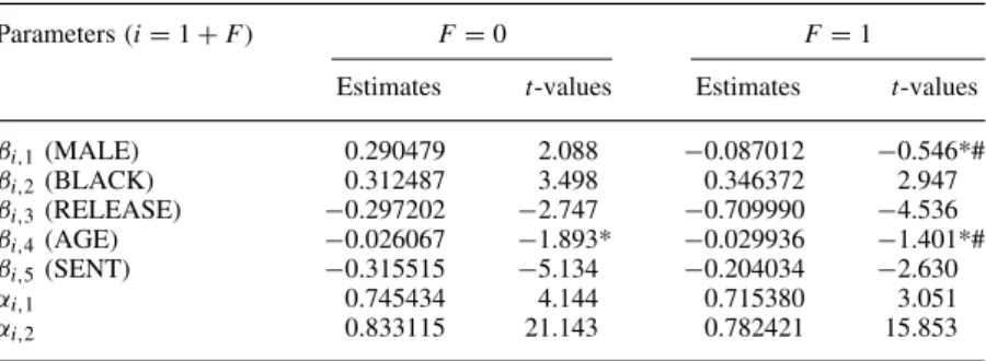
Table VI. ML results for Illinois

Parameters (i_D1_CF) F_D0 F_D1

Estimates t-values Estimates t-values ˇi,1(MALE) 0.290479 2.088 0.087012 0.546*# ˇi,2(BLACK) 0.312487 3.498 0.346372 2.947 ˇi,3(RELEASE) 0.297202 2.747 0.709990 4.536 ˇi,4(AGE) 0.026067 1.893* 0.029936 1.401*# ˇi,5(SENT) 0.315515 5.134 0.204034 2.630

˛i,1 0.745434 4.144 0.715380 3.051

˛i,2 0.833115 21.143 0.782421 15.853

q_D4N_D1090L.L._D 1017.6 ICM test: 0.93. p-value⊲Ł D0⊳D0.10136p-value⊲#D0⊳D0.34518.

decisions and past sentences are (to some extent) determined jointly. If so, the crime type variable

F will not only depend on the past sentence length but also the other way around. However, if this were the case the Logit models for felony arrest would be misspecified, but the ICM tests do not reject either of the models. Therefore, this endogeneity hypothesis is not supported by the data.

Table VII. ML results for Michigan

Parameters (i_D1_CF) F_D0 F_D1

Estimates t-values Estimates t-values ˇi,1(MALE) 0.240017 1.157*# 0.285942 1.735* ˇi,2(BLACK) 0.159765 1.298*# 0.489985 5.374 ˇi,3(RELEASE) 0.624128 3.134 0.027477 0.191*& ˇi,4(AGE) 0.067750 2.831 0.096653 4.485 ˇi,5(SENT) 0.138314 1.804* 0.096984 1.628*&

˛i,1 0.973963 2.687 0.825761 3.358

˛i,2 0.927313 17.292 1.002110 22.417

q_D4N_D1423L.L._D 1591.0 ICM test: 1.06.

p-value ⊲Ł D0⊳D0.07682 p-value ⊲#D0⊳D0.15315. p-value ⊲&D0⊳D0.26486 p-value⊲˛2,2D1⊳D0.96236.

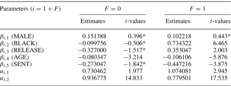
Table VIII. ML results for Minnesota

Parameters (i_D1_CF) F_D0 F_D1

Estimates t-values Estimates t-values ˇi,1(MALE) 0.151388 0.396* 0.102218 0.443* ˇi,2(BLACK) 0.099756 0.506* 0.734322 6.465 ˇi,3(RELEASE) 0.327000 1.517* 0.353047 2.003 ˇi,4(AGE) 0.080347 3.214 0.106106 5.876 ˇi,5(SENT) 0.273047 1.842* 0.447216 3.875

˛i,1 0.730462 1.977 1.074081 2.945

˛i,2 0.936775 14.833 0.779501 17.535

q_D3N_D1220L.L._D 1395.0 ICM test: 1.06. p-value⊲_{Ł D}0⊳_D0.20394.

Table IX. ML results for New Jersey

Parameters (iD1CF) FD0 FD1

Estimates t-values Estimates t-values ˇi,1(MALE) 0.022564 0.148* 0.744489 3.296 ˇi,2(BLACK) 0.391423 3.728 0.415205 3.671 ˇi,3(RELEASE) 0.010225 0.032* 0.216446 0.617* ˇi,4(AGE) 0.090985 4.968 0.160315 7.205 ˇi,5(SENT) 0.206865 1.964 0.192679 1.833*

˛i,1 1.257366 2.312 1.009467 2.027

˛i,2 0.988073 18.898 0.815743 15.652

q_D5N_D1280L.L._D 1450.5 ICM test: 1.54. p-value⊲_{Ł D}0⊳_D0.45476p-value⊲˛1,2D1⊳D0.81955.

Table X. ML results for New York

Parameters (i_D1_CF) F_D0 F_D1

Estimates t-values Estimates t-values ˇi,1(MALE) 0.110116 0.777* 0.696240 3.496 ˇi,2(BLACK) 0.048690 0.493* 0.327048 3.066 ˇi,3(RELEASE) 0.405187 1.936 0.601890 2.394 ˇi,4(AGE) 0.089260 4.765 0.134151 6.288 ˇi,5(SENT) 0.014752 0.228* 0.090108 1.196*

˛i,1 1.153498 3.214 0.988492 2.493

˛i,2 0.892737 19.476 0.889562 16.191

q_D4N_D1365L.L._D 1658.0 ICM test: 1.70.

p-value⊲Ł D0⊳D0.65495p-value⊲˛1,2D˛2,2⊳D0.95605.

Table XI. ML results for Ohio

Parameters (iD1CF) FD0 FD1

Estimates t-values Estimates t-values ˇi,1(MALE) 0.210361 1.373* 0.112386 0.663* ˇi,2(BLACK) 0.372557 3.196 0.971069 7.139 ˇi,3(RELEASE) 0.571839 3.079 0.369154 1.964 ˇi,4(AGE) 0.054033 2.582 0.135771 5.268 ˇi,5(SENT) 0.098486 0.971* 0.252231 1.975

˛i,1 0.197856 3.311 0.319868 2.930

˛i,2 0.678135 14.686 0.888214 12.474

qD3ND1551L.L.D 1753.6 ICM test: 1.44. p-value⊲_{Ł D}0⊳_D0.43364.

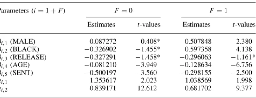
Table XII. ML results for Oregon

Parameters (i_D1_CF) F_D0 F_D1

Estimates t-values Estimates t-values ˇi,1(MALE) 0.087272 0.408* 0.507848 2.380 ˇi,2(BLACK) 0.326902 1.455* 0.597358 4.138 ˇi,3(RELEASE) 0.327291 1.458* 0.296063 1.161* ˇi,4(AGE) 0.081210 3.949 0.128634 6.756 ˇi,5(SENT) 0.500197 3.560 0.298155 2.500

˛i,1 1.353617 2.023 1.038569 1.998

˛i,2 0.839171 12.612 0.681702 9.377

q_D5N_D1017L.L._D 1041.0 ICM test: 1.84. p-value⊲_{Ł D}0⊳_D0.18865.

Apart from the effect of parole in Minnesota and Ohio, the covariates have the expected effect on recidivism. However, what is striking is the heterogeneity of the effects across states, in significance as well as magnitude. In the next section we will have a closer look at the magnitude of the effects of the covariates on recidivism.

4.3. Marginal Quantile Effects

A convenient way to analyze the numerical effect of the covariates on the durationsT1 andT2 is

to fix the marginal conditional survival function to a particular quantile :

1_DP[Ti > tijXDx]DH0⊲exp⊲exp⊲ˇ0ix⊳˛i,1t

˛i,2

i ⊳⊳, iD1,2

which yields a linear relationship between ln⊲ti⊳andx:

ln⊲ti⊳D

ln⊲ln⊲1/u⊳⊳ln⊲˛i,1⊳

˛i,2

1

˛i,2

ˇ0_ix, i_D1,2

where 1_DH0⊲u⊳. Thus, a changex in the vector of covariates results in a relative change

ti ti D

exp 1

˛i,2

ˇ0_ix

1 ⊲20⊳

in the quantile value of ti, regardless the value of . We will call (20) the marginal quantile effect. These effects will be presented below, together with their 95% confidence intervals, in whole percentages. The confidence intervals involved have been computed using the well-known

∂-method.

To highlight the heterogeneity of our empirical results across states, we will present the marginal quantile effects per covariate (Tables XIII–XVII). Clearly, there is substantial variation in the gender effect (Table XIII). For example, in Michigan the time between release and felony arrest is about 25% shorter for males than for females, whereas in New Jersey it is about 60% shorter.

The race effect is even more heterogenous across states than the gender effect, to the point where some confidence intervals do not overlap (Table XIV). For example, this is the case in Illinois and Ohio. In Illinois the time between release and felony arrest is, with probability 95%, between 16% and 55% shorter for African-Americans than for other races, whereas in Ohio this time is between 56% and 77% shorter.

The deterrent of parole or probation is the strongest in Illinois (Table XV). In this state parolees have an almost three times (148%) longer time between release and felony arrest than other ex-convicts, although the 95% confidence interval is wide. As noted before, in Ohio the effect of

Table XIII. Marginal quantile effects of x_DMALE with 95% confidence intervals [a, b]

xD1 State FD0 FD1

100t1

t1 a b 100

t2

t2 a b

California 7 42 28 36 52 19

Florida 41 59 23 28 62 5

Illinois 29 53 6 12 33 56

Michigan 23 57 11 25 49 0

Minnesota 15 83 53 12 63 39

New Jersey 2 29 33 60 82 38

New York 12 39 16 54 74 34

Ohio 27 59 6 12 45 21

Table XIV. Marginal quantile effects of x_DBLACK with 95% confidence intervals [a, b]

x_D1 State F_D0 F_D1

100t1

t1 a b 100

t2

t2 a b

California 9 26 45 55 65 44

Florida 27 43 11 57 71 43

Illinois 31 46 16 36 55 16

Michigan 19 12 50 39 50 27

Minnesota 11 35 57 61 73 49

New Jersey 33 47 19 40 57 23

New York 5 26 15 31 47 14

Ohio 42 62 23 66 77 56

Oregon 48 31 126 58 76 41

Table XV. Marginal quantile effects ofx_DRELEASE with 95% confidence intervals [a, b]

x_D1 State F_D0 F_D1

100t1

t1 a b 100

t2

t2 a b

California N.A. N.A.

Florida 65 27 103 84 25 143

Illinois 43 6 80 148 49 247

Michigan 96 13 179 3 26 32

Minnesota 42 23 106 36 65 8

New Jersey 1 65 63 30 80 140

New York 57 15 130 97 13 206

Ohio 57 79 35 34 61 7

Oregon 48 30 125 54 59 168

parole on both types of arrests is reversed, and in Minnesota the same applies to felony arrest. Parolees in Ohio are about 57% earlier arrested for a misdemeanor and 34% earlier for a felony than other ex-convicts. The latter effect is about the same for Minnesota. A possible explanation for the difference of these effects may be differences in effectiveness of parole officers. If a parole officer has the time to closely monitor his clients, he may observe signs indicating that a parolee is involved in illegal activities (for example, if the parolee shows up in an expensive car), and report this to the police, whereas an overworked parole officer with too many clients may miss these signs. Another explanation may be that the criteria used by parole boards for granting parole vary per state.

Tables XVI and XVII measure the quantile effects of an increase of age by 5 years, and of sentence length by 1 year.11_{Again, there is a substantial variation in age effects, even to the point}

where some 95% confidence intervals do not overlap, for example in the case of felony arrests in California and Florida.

11_{Recall that AGE and SENT are measured in days per 1000, so that an increase by one year corresponds to an increase}

of 0.365 in these variables.

Table XVI. Marginal quantile effects of x_DAGE with 95% confidence intervals [a, b]

x_D5⊲y⊳State F_D0 F_D1

100t1

t1 a b 100

t2

t2 a b

California 30 17 44 22 12 32

Florida 27 19 35 49 34 64

Illinois 6 0 12 7 3 18

Michigan 14 4 25 19 10 29

Minnesota 17 6 28 28 17 39

New Jersey 18 11 26 43 29 58

New York 20 11 29 32 20 44

Ohio 16 3 28 32 18 46

Oregon 19 9 29 41 28 55

Table XVII. Marginal quantile effects of x_DSENT with 95% confidence intervals [a, b]

x_D1⊲y⊳State F_D0 F_D1

100t1

t1 a b 100

t2

t2 a b

California 23 11 35 28 15 41

Florida 7 3 17 21 6 37

Illinois 15 9 21 10 2 18

Michigan 6 1 12 4 1 8

Minnesota 11 1 24 23 10 37

New Jersey 8 0 16 9 1 19

New York 1 6 5 4 3 10

Ohio 5 6 17 11 0 22

Oregon 24 9 39 17 3 31

In quite a few states an increase in the sentence length reduces recidivism, in particular for felonies. The effect is the strongest in California: an increase of the sentence length by 1 year increases the time between release and arrest by about 23% in the case of misdemeanor arrest, and by about 28% in the case of felony arrest. On the other hand, in some states the effect is not significant, in particular in Michigan and New York.

5. CONCLUSIONS

As to the analysis itself, our approach and results are novel in various aspects. The first novelty is the BJS data set itself, which to the best of our knowledge has not been used in this way. Previous research on recidivism has used local data sets. Indeed, the very reason for the Bureau of Justice Statistics to collect this data is the common need in the profession for better data on recidivism (see Maltz, 1984). A lesser novelty is the disaggregation of rearrests in two types: misdemeanor and felony arrests. Since Schmidt and Witte (1988), the econometric approach to the analysis of recidivism has mainly focused on proportional hazard models without distinction between types of crime. An exception is Escarela et al. (2000), but they consider different types of offenses. Consequently, it is not possible to compare our estimation results with similar results in the literature.

Our main methodological contributions are the incorporation of common unobserved heterogene-ity in a semi-nonparametric way, which eliminates possible misspecification of that distribution, and the new approach for testing the validity of the models via the implied Logit models for felony arrest.

ACKNOWLEDGEMENTS

The helpful comments of John Rust and two referees on previous versions of this paper are gratefully acknowledged. This paper is a substantial further elaboration of the first essay of Carvalho’s (2002) PhD dissertation at the Pennsylvania State University. Carvalho’s research was sponsored by the CAPES Foundation, Brazil.

REFERENCES

An MY, Christensen BJ, Datta Gupta N. 2004. Multivariate mixed proportional hazard modelling of the joint retirement of married couples.Journal of Applied Econometrics19: 687 –704.

Andrews DWK, Ploberger W. 1994. Optimal tests when a nuisance parameter is present only under the alternative.Econometrica62: 1383 –1414.

Barton RR, Turnbull BW. 1981. A failure rate regression model for the study of recidivism. In Models in Quantitative Criminology, Fox JA (ed.). Academic Press: New York; 81 –102.

Beck AJ, Shipley BE. 1989. Recidivism of prisoners released in 1983. Special report, Bureau of Justice Statistics.

Bierens HJ. 1982. Consistent model specification tests.Journal of Econometrics20: 105 –134.

Bierens HJ. 1990. A consistent conditional moment test of functional form.Econometrica58: 1443 –1458. Bierens HJ. 2006a. EasyReg International. Free econometric software. http://econ.la.psu.edu/¾hbierens/

EASYREG.HTM.

Bierens HJ. 2006b. Review of the integrated conditional moment test and its implementation in EasyReg International. http://econ.la.pus.edu/¾hbierens/ICMMEAN.PDF.

Bierens HJ. 2006c. Semi-nonparametric interval censored mixed proportional hazard models: identification and consistency results. Forthcoming inEconometric Theory. http://econ.la.psu.edu/¾hbierens/SNPMPHM. PDF.

Bierens HJ, Carvalho JR. 2006. Separate appendix to: Semi-nonparametric competing risks analysis of recidivism. http://econ.la.psu.edu/¾hbierens/RECIDIVISM APP.PDF.

Bierens HJ, Ploberger W. 1997. Asymptotic theory of integrated conditional moment tests. Econometrica

65: 1129 –1151.

Blumstein A, Cohen J. 1979. Estimation of individual crime rates from arrest records.Journal of Criminal Law and Criminology 70: 561 –585.

Boning WB, Sowell F. 1999. Optimality for the integrated conditional moment test.Econometric Theory15: 710 –718.

Carr-Hill GA, Carr-Hill A. 1972. Reconviction as a process.British Journal of Criminology 12: 35 –43. Carvalho JR. 2002. Essays on the microeconometrics of labor markets and criminal behavior. PhD thesis,

Pennsylvania State University.

Chung CF, Schmidt P, Witte A. 1991. Survival analysis: a survey.Journal of Quantitative Criminology 7: 59 –98.

Copas JB, Heydari F. 1997. Estimating the risk of reoffending by use of exponential mixture models.Journal of the Royal Statistical Society Series A160: 237 –252.

Escarela G, Francis B, Soothill K. 2000. Competing risks, persistence, and desistance in analyzing recidivism. Journal of Quantitative Criminology 16: 385 –414.

Gendreau P, Little T, Goggin C. 1996. A meta-analysis of the predictors of adult offender recidivism: What works!Criminology 34: 575 –607.

Hannan EJ, Quinn BG. 1979. The determination of the order of an autoregression. Journal of the Royal Statistical Society Series B 41: 190 –195.

Hausman JA. 1978. Specification testing in econometrics.Econometrica46: 1251 –1271.

Heckman JJ, Honore BE. 1989. The identifiability of the competing risks model.Biometrika 76: 325 –330. Hougaard P. 1987. Modelling multivariate survival.Scandinavian Journal of Statistics 14: 291 –304. ICPSR. 1989. Recidivism among released prisoners, 1983. Discussion Paper 8875, Inter-university

Consor-tium for Political and Social Research, Ann Arbor, MI.

Imai S, Krishna K. 2004. Employment, deterrence and crime in a dynamic model.International Economic Review 45: 845 –872.

Maltz MD. 1984.Recidivism. Academic Press: New York.

Partanen J. 1969. On waiting time distributions.Acta Sociologica 12: 132 –143.

Rhodes W. 1986. A survival model with dependent competing events and right-hand censoring: probation and parole as illustration.Journal of Quantitative Criminology 2: 113 –137.

Schmidt P, Witte AD. 1988.Predicting Recidivism Using Survival Models. Springer: New York.

Schmidt P, Witte AD. 1989. Predicting criminal recidivism using ‘split population’ survival time models. Journal of Econometrics 40: 141 –159.

Schwarz G. 1978. Estimating the dimension of a model.Annals of Statistics6: 461 –464.

Stinchcombe MB, White H. 1998. Consistent specification testing with nuisance parameters present only under the alternative.Econometric Theory 14: 295 –325.

Stollmack S, Harris CM. 1974. Failure rate analysis applied to recidivism data. Operations Research 23: 1192 –1205.

Van den Berg G. 2000. Duration models: specification, identification, and multiple duration. Handbook of Econometrics, Vol. V. North-Holland: Amsterdam.

Visher CA, Linster RL. 1990. A survival model of pretrial failure.Journal of Quantitative Criminology 6: 153 –184.

Wooldridge JM. 2001. Asymptotic properties of weighted m estimators for standard stratified samples. Econometric Theory 17: 451 –470.