1
ESTIMATION OF COST ALLOCATION COEFFICIENTS AT THE FARM LEVEL USING AN
ENTROPY APPROACH Maria Leonor da Silva Carvalho (apresentador)
(Universidade de Évora, ICAAM/CEFAGE, Évora, Portugal, leonor@uevora.pt)
Pery Francisco Assis Shikida
(UNIOESTE-Toledo, Brasil, peryshikida@hotmail.com)
Rui Manuel de Sousa Fragoso
(Universidade de Évora, CEFAGE/ICAAM, Évora, Portugal, rfragoso@uevora.pt)
Weimar Freire da Rocha Jr
(UNIOESTE-Toledo, Brasil, wrochajr2000@gmail.com)
Abstract
This paper aims to estimate the farm cost allocation coefficients from whole farm input costs. An entropy approach was developed under a Tobit formulation and was applied to a sample of farms from the 2004 FADN data base for Alentejo region, Southern Portugal. A Generalized Maximum Entropy model and Cross Generalized Entropy model were developed to the sample conditions and were tested. Model results were assessed in terms of their precision and estimation power and were compared with observed data. The entropy approach showed to be a flexible and valid tool to estimate incomplete information, namely regarding farm costs.
Keywords: Generalized maximum entropy; costs; estimation; Alentejo, FADN.
2
ESTIMATION OF COST ALLOCATION COEFFICIENTS AT THE FARM LEVEL USING AN
ENTROPY APPROACH
1 - Introduction
Detailed information on production costs at the farm level is particularly important, both from a business management and agricultural-policy perspective. Farm level responses to changes in markets and technologies and agricultural and environmental policies are often assessed by using farm costs disaggregated per input type and output activity. According to Lips (2009), farm input costs per output activity are crucial to farming decisions due the following three reasons. First, they are essential to calculate the output profits and returns to resources. Second, the shares of different groups of input costs on the total cost give an insight of the cost structure of each output activity, helping on management decisions. Finally, they allow comparisons among technologies, farms, regions and even at international level.
Usually this kind of data is not available. Most farms do not have detailed accounting data, and this calculation of input costs per output is not possible. Universities have been collecting and treating some information on input-output technical coefficients and costs. Nevertheless, these data are based either on the results of field experiments or are limited to specific areas. The Farm Accountancy Data Network (FADN) provides detailed accounting data at the farm level. However the costs per input type are presented only for the whole farm, without revealing the distribution of production costs by the various output activities.
The costs per output activity can be obtained either from collecting data directly in farms, or through estimated coefficients of input costs from samples of FADN data base. The second approach seems to be the best solution, since the first approach is expensive and too demanding in resources.
There are several works that estimate crop-specific inputs (Just et al., 1983; Shumway et al., 1984; and Lence and Miller, 1998a e 1998b). Most of them are based on the relationship between input allocations and production coefficients under the assumption of profit maximization. Traditionally the tools used in these approaches are linear regression techniques (LRT), Bayesian estimation techniques (BES) and linear programming (LP), but their use raises some practical concerns.
In the problem of farm cost allocation, it is necessary to ensure the accounting balance between total revenue and total costs. In this situation the disturbance terms of the various input-demand equations are not independent from each other and the system
3 of input-demand equations is singular, which invalidates the use of LRT techniques (Bewley, 1986). Another well known result of the LRT technique is the negative input-demand coefficients that could be estimated. This can be avoided by using BES techniques or inequality least squares methods (Moxey and Tiffin, 1994). However, the application of these alternative methods is heavy and does not allow incorporating the accounting constraints which need to be treated separately in the system. A flexible alternative that has been widely applied to estimate farm input and output coefficients is the entropy approach. This methodology does not require behavioural assumptions and allows the use of non sample information through the introduction of information priors. This paper aims to apply a flexible methodology that allows estimating the coefficients of farm cost allocation per output activity from the whole farm input costs, taking into account general conditions of Mediterranean areas. An entropy approach is used to make the estimation of coefficients at the farm level based on a farms sample of the FADN data base in the Alentejo region, South of Portugal. A Generalized Maximum Entropy (GME) model and a Cross Generalized Entropy (CGE) model are applied and assessed by looking at the precision of the coefficients extracted from the whole farm data and comparing them with the observed input-output coefficients. In Portugal as well as in Mediterranean areas, there are few studies that estimate coefficients of farm cost allocation, being this study the first one done on this issue in Portugal.
This paper is organized in five additional sections. Section 2 presents the entropy approach. Section 3 describes the analytical framework developed to estimate the input cost coefficients. Section 4 reports the data used. Section 5 presents and discusses the results and section 6 provides the conclusion.
2 – The entropy approach background
Lence and Miller (1998a) proposed a GME approach for simultaneously estimating multi-output production function and recovering input allocations. This approach was also used by Zhang and Fan (2001) to estimate crop-specific production technologies in Chinese agriculture. Leon et al. (1999) and more recently Peeters and Surry (2005) used maximum entropy and FADN data base to derive farm crop coefficients in Brittany, France. Garvey and Britz (2002) estimated agricultural input allocation from EU farm accounting data. Hansen and Surry (2006) estimated input quantities for different production branches based on regional economic accounts.
4 Fragoso et al. (2008) applied a CGE model to conduct a dynamic disaggregation of spatial information in the Alentejo region.
The main issues on the theoretical background of the entropy approach can be found in Shannon (1948), Jaynes (1957a; 1957b), Kullback (1959), Gokhale and Kullback (1978), Levine (1980), Jaynes (1984), Csiszár (1991) and Golan et al. (1996a).
The concept of entropy was introduced by Shannon (1948) in the context of the information theory as a measure of uncertainty. The Shannon’s entropy measure is given by the relation ( ) ∑ ( ) with k =1,..,K and where pk is the probability of observing outcome k. Under this concept the information contained in one observation k of a random event has an inverse relationship with its probability, being the maximal information generated when pk value is 1/K. To assign or recover the unknown probabilities pk, Jaynes (1957a; 1957b) propose the maximum entropy (ME) principle:
( ) ∑ ( ) ( )
∑ ∑
Given the independent random variable yk and the moment of its distribution the dependent variable x, this formulation allows us to choose pk ={p1,p2,…,pk} that maximizes the entropy function H(p) taking into account t=1,2,...,T constraints of information-moment relations, the adding-up constraints and the non-negativity conditions. According to the ME principle, there is a unique probability distribution that maximizes Shannon’s entropy measure and is consistent with the available information contained in the data. The selected probability distribution is the one that, among others, satisfies the condition of information consistency, with the minimum information content.
The GME approach proposed by Judge and Golan (1992) generalizes the ME principle and allows to treat the noisy component of the linear regression. The unknown parameters αk and the unknown errors et are written as the expected value of a probability distribution, defined over the sets of the known and discrete “support values” zkm and vtn (Golan and Judge, 1996 and Golan et al., 1996a):
5 ∑ [ ] [ ] ( ) ∑ [ ] [ ] ( )
The GME estimator αk can be viewed as a random variable with M ≥ 2 outcomes, resulting from the product of the unknown (KM×1) probability vector p by the (K×KM) matrix of support points z. These points are related with exogenous parameters which are based on previous information (Fraser, 2000; Campbell and Hill, 2005 and 2006; and Pires et al., 2010). The error estimate is done in a similar way, considering N ≥ 2 support points, the known (T×TN) matrix of the support points v and the unknown (TN×1) vector of error probabilities w.
According to Golan et al. (1996a) the choice of support bounds for parameters z and errors v has important implications on the estimates. The support bounds can be either symmetric or asymmetric, depending on the characteristics of the data information. Usually as the width of support bounds increases the impact of the information contained in the data grows and decreases the role of the support vector on the results.
Regarding to the support bounds of error terms the most common is the use of the 3σ rule, under the assumption that the error terms have mean zero and variance σ2
. According to this rule the support vector is centered at the origin and its bounds are three times the standard deviation from the origin (Golan et al., 1996a; Peeters and Surry, 2002; and Pires et al., 2010). Since σ is unknown, it can be estimated either using the ordinary least square regression or calculating the sample standard deviation of xt.
Under the GME formulation the model can be written in the matrix form as follows:
( ) ( ) ( ) ( ) s.t. ( ) ( ) ( ) ( ) ( ) where x, y, z and v are known, p and w are the unknown vectors to be estimated and is the Kronecker product. The objective function (4) maximizes the entropy assuming independence between p and w vectors and is subject to data constraints (5) and
adding-6 up (6) constraints, which assure that the probabilities sum is equal to one for each K parameters and T errors
Solving the first order conditions of the Lagrangian function, ̂ and ̂ are given by:
̂ ( ̂ )
∑ ( ̂ ) ( ) ̂ ( ̂ )
∑ ( ̂ ) ( ) The exponential forms guarantee that estimates values of parameters are always positives. The vector ̂ is the vector of unknown Langrange multipliers for data constraints that is associated to the optimal solution of ̂ and ̂ . This vector incorporates the F( ̂ ) information matrix that is given by the following Hessian matrix of the objective function:
( )( ) ( ) [ ] ( ) where is a positive definite matrix for p>0 and w>0 which satisfies the sufficient condition for strict convexity, assuring this way that the solution of the problem is unique.
The entropy approach allows us to incorporate in the estimation any additional information from previous observations through the Cross Entropy principle (CE) introduced by Good (1963). This framework is very useful to reach better estimates and its objective is the minimization of the discrepancy between the posterior probability estimates pk and priors of information qk. The CE minimization problem can be written as follows:
( ) ∑ ( ) ( )
∑ ∑
where pk={ p1, p2,… pK,} is the unknown probability vector to estimate and qk={ q1, q2,… qK,} is the known prior information vector.
The CE entropy principle can also be formulated as a Generalized Cross Entropy (GCE) framework. This was introduced by Golan et al. (1996a) and as the GME it is an extension of its original entropy principle which allows taking into account the expected values of unknown distributions and measurement of error components.
7
3 - Estimates analytical framework
The estimation of cost allocation coefficients from whole farm accounting data is often based on the derived demand of each farm input as a function of several farm outputs. In this formulation inputs and outputs are both expressed as costs and revenues in a system of linear equations, where they are treated respectively as dependent and independent variable.
Considering I inputs types, a sample of T farms producing K outputs, the estimation problem of cost allocation coefficients expressed as a system of linear equations can be written as follows:
∑
( ) where is the cost by farm t and input i; is the unknown cost allocation coefficient by farm output k and input i; is the production value of output activity k in farm t; and is the noisy component specified by input i and by farm t.
This problem can be treated by developing an analytical framework based on an entropy approach. Like Peeters and Surry (2002), a GME model was developed to the conditions of a sample of farms from FADN data base in the Alentejo Region. This model takes into account only crops due to information data constraints. This model takes into account only crops due to information data constraints, and to avoid that some costs may be zero, because not all crops in all farms are observed, the GME model adopts a Tobit formulation as recommended by Golan et al. (1996a) and Peteer and Surry (2002), under which the observations are ordered as follows:
[ ] [ ] [ ] ( ) Thus considering the problem of cost allocation coefficients formulated in (11) the GME-Tobit model can be represented by the following relations:
( ) ∑ ∑ ∑ ( ) ∑ ∑ ∑ ( ) ∑ ∑ ∑ ( ) ( ) s.t. ∑ ∑ ∑ ( )
8 ∑ ∑ ∑ { } ( ) ∑ ( ) ∑ ( ) ∑ ( ) ∑ ∑ ∑ ( ) where T1 are the farms with positive observations and T2 are the farms with zero observations for input i.
Thus, given the known support vectors , , and and the data sample on inputs and outputs , the model finds the positive probability vectors , and
The data consistency constraints (14)-(15) treat the relations in equation (11) as an interdependent system of equations in which all inputs i are taken in account simultaneously and positive and null observations are separated. These constraints guaranty, in the optimization model, the balance between total costs and revenues. Equations (16)-(18) are the adding-up constraints that are related with the probability properties and make in the model the normalization of the probability values of and concerning the dimensions M and N, respectively. In this case, it is also necessary to impose the accounting restriction ∑ for all k in the equation (19), which ensures that the sum by each input i of the probability vectors , weighted by the support vector of dimension M, is equal to 1 for all k. Thus, the accounting balance between total revenue and total cost is always satisfied.
The Ministry of Agriculture has calculated the standard gross margin for the main crops in all agrarian Portuguese regions until 2004. The cost structure that has been utilized can be used as prior information considering the following CGE formulation, subject to the same constraints that in the above GME formulation:
9 ( ) ∑ ∑ ( ) ∑ ∑ ∑ ( ) ∑ ∑ ∑ ( ) ( ) The model minimizes the distance between the estimates of unknown and the previous out sample known information which is used to bring model results closer to the observed data.
Golan et al. (1996a and 2001) studied the properties of the ME estimators of constrained and unconstrained system of equations. If the ME estimators are consistent and asymptotically normal, it is possible to show that the entropy ratio statistic (ER) for different parameters of unknown distribution has a limiting distribution (Peeters and Surry, 2002).
Models are assessed studying statistical proprieties of the estimated parameters as information content and predict power. Then their values were compared with observed data and the proportion of heterogeneity information recovered was assessed. The information content in the estimates can be assessed using the normalized entropy (Golan et al., 1996a, and 1996b). The entropy reaches its maximum value if the uncertainty is also maximal, which is obtained when the information moment constraints are unrestricted and the distribution of probabilities is uniform over all states. Any information added will reduce the uncertainty and the proportion of the remaining uncertainty is measured by:
( ̂) ∑ ∑ ∑ ̂ ( ̂ )
( ) ( ) where S( ̂) is the normalized entropy and its values can vary between zero and one; and
I×K is the total number of coefficients that have to be estimated considering M support
values.
Before adding any information or theoretical constraint the uncertainty is maximal, the value of is 1/M and the entropy of its probability distribution is ln(M). For the K×I joint entropy the maximum value is equal to IKln(M) and S( ̂) When S( ̂) , there is no uncertainty and the information content on estimates from the data is maximal.
The normalized entropy indicator for the probability distributions associated to the error terms w1 and w2 can also vary between zero and one and is calculated as:
10 ( ̂) [∑ ∑ ∑ ̂ ( ̂ ) ̂ ( ̂ )]
( ) ( ) The “pseudo R2”, was used to assess the predict power of the tobit model, and was defined as the square of the correlation between predicted and observed values for each input cost as in Peeters and Surry (2002):
[∑ ̂ ]
[∑ ̂ ̂ ] ̂ ∑ ̂ ( ) where ̂ are the estimated values of inputs costs. The closer R2 is to one, the better is the predictive power of the model.
The model validity was assessed comparing the estimated cost allocation coefficients ̂ with the observed coefficients , by using the Percentage of Absolute Deviation (PAD) computed by crop k and input i and the Weighted Percentage of Absolute Deviation (WPAD) by crop k:
| ̂ | (24) (25) where is the i input cost per crop k and is the total cost per crop k. The observed coefficients were obtained crossing the data sample with the structure of input costs per crop which results from the standard gross margin calculation made by the Portuguese Ministry of Agriculture. The WPAD is another useful indicator to measure the prediction errors that weight the PAD by the share of each input cost in the total per crop.
The proportion of heterogeneity that is recovered by the model was measured through the disaggregate information gain (DIG) indicator developed by Howitt and Reynaud (2003): ̂ ∑ ∑ ̂ (̂ ) ∑ ∑ ( ) (26) This measure is based on the cross entropy between the coefficients ̂ and and on the cross entropy between the aggregated coefficients and the disaggregated coefficients . In the case of a perfect information recovery the DIG is equal to one, meaning that 100% of the information contained on the data was recovered.
11
4 – Empirical data
The data used were from the 2004 FADN database for the Alentejo region which contains general information by farm, such as production value, surface of crops, livestock units and input costs. Production value is defined in euros by output activity (crops and livestock). Crops acreage is presented in hectares and livestock in heads. The costs are disaggregated by item, but are aggregated for the whole farm and we cannot know directly from the data the costs per output activity.
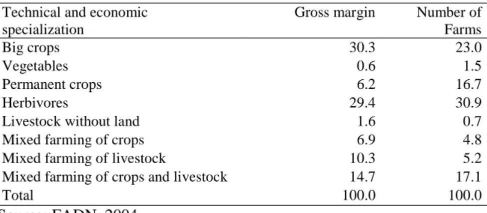
Table 1 presents the distribution of gross margin and number of farms by technical and economic specialization branch in the Alentejo region according to 2004 FADN database.
Table 1. Percentage of gross margin and number of farms in Alentejo Technical and economic
specialization
Gross margin Number of Farms
Big crops 30.3 23.0
Vegetables 0.6 1.5
Permanent crops 6.2 16.7
Herbivores 29.4 30.9
Livestock without land 1.6 0.7
Mixed farming of crops 6.9 4.8
Mixed farming of livestock 10.3 5.2
Mixed farming of crops and livestock 14.7 17.1
Total 100.0 100.0
Source: FADN, 2004
The technical and economic specialization branches of big crops, herbivores and mixed farming of crops and livestock have almost 75% of the regional gross margin. These three technical and economic specialization branches and permanent crops are also the most representative regarding the number of farms (88%).
Given these data characteristics, a convenient sample of 30 farms was extracted from the 2004 FADN database. Due to methodological and data limitations this sample includes farms that have only output crop activities, 24 farms from big crops branch (80%) and 6 farm from permanent crops branch (20%). The first covers 30.3% of the Alentejo gross margin and 23% of farms, and the second covers 6.2% and 16.7%, respectively. Therefore the sample represents almost 40% of the regional gross margin and number of farms.
The sample includes 8 output crops and 5 cost items. Crops are wheat, maize, rice, other cereals, horto-industrials and melons, oilseeds, olive trees and vineyards, and represent an important share of agricultural production in the Alentejo region. According to the methodology used by the Ministry of Agriculture to calculate the
12 standard gross margins, the item costs that were considered are plants and seeds, fertilizers, pesticides, other costs with crops and gross margin.
Table 2 presents the main characteristics of the sample, such as, mean, maximum and minimal values of production, acreage and cost items.
Table 2. Characteristics of farm data sample
Source: FADN, 2004
Most of the production value is allocated to vineyards (40%) and horto-industrial (34%). Their mean and maximum values are €25,107 and €21,269, and €522,302 and €352,769, respectively. However, the acreage shares are low. Vineyards represent only 5% of the total acreage and horto-industrials are 9%.
The maize is the third crop in the share of production value (10%). Its mean is €6,089 and the maximum reach to €107,384. The acreage (7% of total) is less than the acreage of wheat (38%), oilseeds (14%) and other cereals (16%), which have lower production values.
Regarding cost items, gross margin represents 63% of total production value. The mean and maximum values are the highest among cost items, €39,581 and €440,767, respectively. Unlike the other sample elements that have as minimum value zero, for the gross margin this is negative (€6,012). The cost items of fertilizers, other costs, pesticides and seeds and plants, are 11.8%, 9.2%, 8.6% and 7.5% of total
Mean Maximum Minimum Percentage
Production value (Euros)
Wheat 3331 12308 0 5.3 Maize 6089 107384 0 9.7 Rice 1930 22899 0 3.1 Other cereals 2752 47276 0 4.4 Horto-industrials 21269 352796 0 33.8 Oilseeds 954 13398 0 1.5 Olive trees 1480 12833 0 2.4 Vineyards 25107 522302 0 39.9 Acreage (ha) Wheat 19.3 67.0 0 38.0 Maize 3.6 47.3 0 7.0 Rice 2.1 21.5 0 4.1 Other cereals 8.1 78.4 0 16.0
Horto-industrials and melon 4.5 5.0 0 8.8
Oilseeds 6.9 55.0 0 13.7
Olive trees 3.6 24.9 0 7.2
Vineyards 2.6 28.7 0 5.2
Item costs (Euros)
Seeds and plants 4715 40301 0 7.5
Fertilizers 7437 71573 0 11.8
Pesticides 5388 55105 0 8.6
Other costs 5791 81821 0 9.2
13 production value, respectively. Among them, the mean varies between €4,715 in seeds and plants and €7,437 in fertilizers and the maximum value varies from €40,301 in seeds and plants to €81,821 in other costs.
For vineyards, maize, other cereals and horto-industrials the maximum production value is greater than the mean almost twenty times. Regarding cost items, these differences are smaller, and vary from 8.5 times in seeds and plants to 14 times in other costs with crops.
5 – Results
For the estimation of cost allocation coefficients two model specifications were used, a GME-tobit and a CGE-tobit formulation, under the sample of 30 farms from the Alentejo 2004 FADN database using the GAMS (General Algebraic Modeling System) software. Results are presented in terms of the precision estimates and prediction power, and then, a discussion about its validation is done.
The GME-Tobit model requires the choice of the support vectors z and v of dimension M and N which are uninformative uniform distributions to be considered as priors when any prior information is not available (Howitt and Reynauld, 2003). Several studies have shown that GME estimates are fairly sensitive to the choice of the bounds of the support values, particularly regarding the error terms (Fraser, 2000; Leon et al., 1999; Paris and Caputo, 2001; Preckel, 2001; and Huang et al., 2007).
In the GME formulations, the bounds of the error term are defined as some multiple of the standard deviation of the dependent variable (Golan, et al. 1996b). In this case, the two error support vectors (v1 and v2) were defined with the center on zero and the endpoints of interval [ ] based on the “3σ rule” (Pukelsheim, 1994). The σ is obtained assuming a uniform and censored distribution of the data where the uniform variance (s2) is used as an estimator of σ (Golan et al., 1997). For the parameters support vector z the natural bounds are zero and one and M is equal to 3. Like Fragoso et al. (2008), Martins et al. (2011) and Howitt and Reynauld (2003) the set of support values considered was {0.0, 0.5, 1.0}.
In the CGE-Tobit formulation the parameters and error supports z, v1 and v2 were defined in the same way as the GME-Tobit model, considering for the error term the three sigma rule and for z the symmetric set of {0.0, 0.5, 1.0}. The exogenous information prior ( ) that was used regarding the coefficients of production value and
14 costs structure used by Portuguese Ministry of Agriculture to calculate the standard gross margin in 2004.
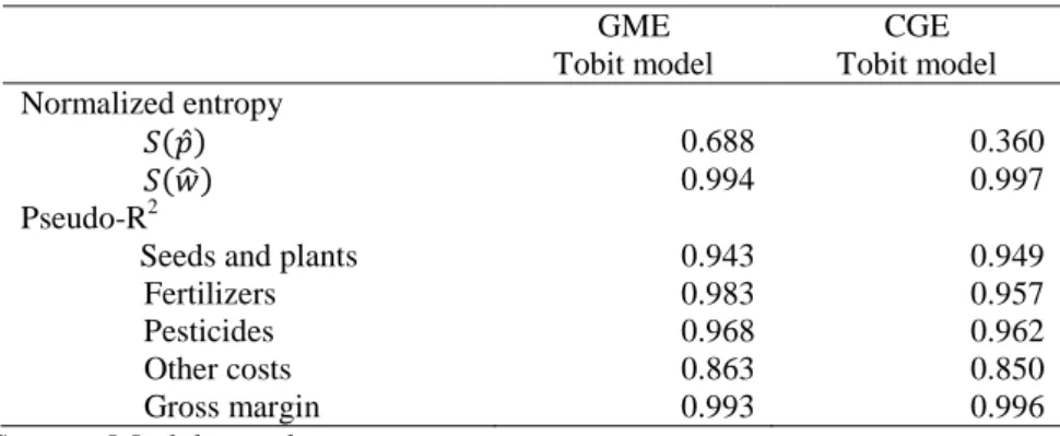
Table 3 presents the model results for indicators of precision and prediction power, with respect to the normalized entropy for the estimates of parameters ( ̂) and of the error ( ̂) and the pseudo-R2
.
Table 3. Indicators of model precision and prediction power
GME Tobit model CGE Tobit model Normalized entropy ( ̂) 0.688 0.360 ( ̂) 0.994 0.997 Pseudo-R2
Seeds and plants 0.943 0.949
Fertilizers 0.983 0.957
Pesticides 0.968 0.962
Other costs 0.863 0.850
Gross margin 0.993 0.996
Source: Models results
The normalised entropy assesses the information content in a model measuring the remaining uncertainty, which gives the amount of new information that is generated by the entropy estimators. The ( ̂) indicator shows that the amount of new information generated is 0.688 in the GME model and 0.36 in the CGE model. As expected the GME model generate more new information than the CGE model. In this last the importance of data on the estimates is greater due to the influence of the information prior on the model results and the uncertainty of the estimates is lower than in GME model. For both models the noise ratios S( ̂) are high meaning that almost of all distribution error is recovered by the new information generated in estimation process.
The “pseudo R2“ statistic was calculated for each input or cost item and was used to assess the predictive power of the models. For all cost items, the “pseudo R2“ is close to one. The item having the lower results is “other costs”, where the “pseudo R2“ is 0.85 and 0.863. For the other items, the “pseudo R2“ is always above 0.94, being greater than 0.99 in the case of gross margin.
In general the estimates of the GME and CGE model specifications have a good degree of precision and prediction power. These results are similar to the ones obtained by other authors (Peeters and Surry, 2002).
Table 4 shows the estimated cost allocation coefficients and the results of the comparison with observed values given by the calculation of the percentage of absolute deviation (PAD).
14
Table 4. Parameters estimates and percentage of absolute deviation Seeds and Plants Fertilize rs Pesticid es Other costs Gross margin
PAD PAD PAD PAD PAD WPAD
GME – Tobit model
Wheat 0.196 26.9 0.204 32.5 0.196 25.6 0.197 0.0 0.207 21.0 27.0 Maize 0.120 2.4 0.223 139.8 0.190 10.0 0.183 33.0 0.283 5.7 26.1 Rice 0.192 269.2 0.200 11.1 0.201 337.0 0.200 32.4 0.208 45.4 58.9 Other cereals 0.160 6.4 0.214 970.0 0.212 61.8 0.190 24.3 0.224 47.4 57.7 Horto industrials 0.115 210.8 0.213 117.3 0.161 85.1 0.073 17.7 0.439 38.8 55.6 Oilseeds 0.189 361.0 0.204 0.0 0.203 4.1 0.197 18.0 0.207 65.3 59.3 Olive trees 0.197 380.5 0.201 458.3 0.197 0.0 0.200 0.0 0.204 77.6 101.2 Vineyard 0.020 47.4 0.048 51.5 0.033 0.0 0.185 0.0 0.714 16.9 17.3
CGE – Tobit model
Wheat 0.320 19.4 0.189 37.4 0.208 33.3 0.009 0.0 0.273 4.2 24.0 Maize 0.093 24.4 0.140 50.5 0.200 5.2 0.178 34.8 0.390 30.0 27.0 Rice 0.076 46.2 0.136 39.6 0.078 69.6 0.260 12.2 0.449 17.8 24.9 Other cereals 0.161 5.8 0.017 15.0 0.186 42.0 0.182 27.5 0.454 6.6 16.3 Horto industrials 0.101 173.0 0.186 89.8 0.140 60.9 0.019 69.4 0.554 22.7 41.1 Oilseeds 0.044 7.3 0.000 0.0 0.254 30.3 0.120 28.1 0.582 2.5 12.1 Olive trees 0.050 22.0 0.019 47.2 0.000 0.0 0.010 0.0 0.921 1.1 3.5 Vineyard 0.006 84.2 0.013 86.9 0.000 0.0 0.110 0.0 0.871 1.4 2.6
15 In general the GME model results show important differences between estimated and observed coefficients. Half of the estimated parameters by item cost and crop ( ) have a PAD value above 30%. The WPAD values show that only three crops present acceptable parameter estimations, the wheat, maize and vineyard. In these cases the WPAD is 27%, 26% and 17.3%, respectively. For the first two crops the estimated parameters have in general low PAD values, which range between 0% and 33%. Only the item cost of fertilizers in the maize has a huge PAD value (139.8%). For the vineyard the PAD value is zero in the item costs of pesticides and other costs and is 17.3% in case of gross margin.
For the remaining crops, the values of WPAD are above than 55% and the item costs that have the more troubled PAD values, are seeds and plants, fertilizers and gross margin. In the first case the PAD values of four crops (rice, horto-industrial and melon, oilseeds and olive trees) are greater than 200%. For fertilizers the PAD value reaches to 970% and 458% in cases of other cereals and olive trees.
The huge deviations of the estimated parameters from the observed coefficients can be explained in large part because the sample of the farms chosen has a great heterogeneity, and we have assumed in the estimation procedure that all farms operate with the same technology and have the same level of efficiency. In some way this result was predictable when we analyzed the data of table 2 about the characteristics of the farm sample, namely the great differences that exists among the mean, maximum and minimum values of crop revenues and cost items.
The CGE model results are more close to the observed farm cost allocation coefficients than those of the GME model. The average WPAD is 31.4% which is much lower than 101% that was obtained in the GME model.
In the CGE model 35% of the estimated parameters have PAD values below 10% and almost 60% are less than 30%. The WPAD per crop present values below 5% in the vineyard (2.6%) and olive trees (3.5%) and are less than 25% for the remaining crops with the exception of oilseeds, which the WAPD value is 41%.
The most worrying values of the estimated parameters are obtained for the cost items of fertilizers and pesticides, namely for the rice and horto-industrials, which PAD values vary between 39.6% and 89.8%. For both crops the PAD values are also high in the case of the seeds and plants cost item. In general, the other results obtained for the PAD values of seeds and plants, other costs and gross margin are acceptable.
16 The results of CGE model allow conclude that it can be used to estimate farm cost allocation coefficients from the FADN database in the conditions of the Alentejo region, southern of Portugal, as well as in many farms of the Mediterranean area.
As in the GME model, the differences between the estimated and observed parameters can be explained in large part by the data characteristics, namely the fact that we have considered the assumption that all farms operate with the same technology and efficiency level. However the deviations on estimates are less in the CGE than in GME formulation due to the introduction in the model of out sample prior information about the cost coefficients that are used by the Portuguese Ministry of Agriculture to calculate the crops standard gross margin.
The results of DIG indicator show that GME model recovers 91.5% of the heterogeneity of disaggregated information. Due to the use of information prior in the estimates, DIG is bigger in the CGE model, reaching 99.6% of heterogeneity recovered.
The both model specification, the GME and CGE, produce estimators that have good statistical and econometric properties as the normalized entropy and and “pseudo-R2“ indicators show. However the GME estimators are far from the observed coefficients and they only can be acceptable to be used to estimated farm input costs per output activity if we consider some out sample prior information under a CGE formulation. Thus results suggest that entropy approach is a good alternative to the traditional methods to estimate cost allocation coefficients and is a very useful tool to deal with incomplete information concerning economic problems.
6 – Conclusion
Standard farm-accounting information is typically restricted to aggregate or whole farm input expenditures, without revealing production costs per output activity. Considering that the direct collection of data is difficult and requires costly farm surveys, alternative tools based on econometric techniques may offer an attractive alternative for obtaining reliable estimates at a significantly lower cost. In this context maximum entropy approaches have been widely used.
A Generalized Maximum Entropy model and a Cross Generalized Entropy Model were used to estimate farm cost allocation coefficients per output crop activity at the farm level from a sample of thirty farms extracted from the 2004 FADN database of Alentejo Region. Model results were assessed looking at the precision and prediction
17 power of estimates and at its real validity comparing them with the observed data. Several interesting conclusions were achieved.
The entropy estimators show good statistical and econometric proprieties regarding the degree of precision and prediction power assessed by the normalized entropy and “pseudo-R2” indicators, respectively.
However the Generalized Maximum Entropy results are far from the observed coefficients, probably due to the great heterogeneity of farms chosen for the sample and which is associated with differences in the production technologies and therefore on the farm efficiency levels. The reliability of the Generalized Maximum Entropy model estimates can be improved using out sample prior information, as the cost structure that was used by the Portuguese Ministry of Agriculture to calculate the standard gross margins, and a Cross Generalized Entropy model specification.
For both models the disaggregation information gains are very relevant and allow recovering the most part of the information heterogeneity contained in data.
The entropy approach showed to be an important and flexible tool for helping in the economic analysis. This is quite important in the estimates of incomplete information, as in the problem of agricultural economics regarding cost allocation coefficients to output activities.
References
Bewley, R. (1986) Allocation Model: Specification, Estimation and Applications. Cambridge: Ballinger Publishing Company.
Campbell, R., and Carter Hill, R. (2006) Imposing parameters inequality restrictions using the principle of maximum entropy. Journal of Statistical Computation and
Simulation, 76, 985-1000.
Campbell, R., and Carter Hill, R. (2005) A Monte Carlo study of the effect of design characteristics on the inequality restricted maximum entropy estimator. Review of
Applied Economics, 1, 53-84.
Csiszár, L. (1991) Why Least Squares and Maximum Entropy? An Axiomatic Approach to Inference for Linear Inverse Problems. The Annals of Statistics, 19, 2032-2066 Fragoso, R., Martins, M.B., and Lucas, M.R. (2008) Disaggregated soil allocation data using a Minimum Cross Entropy Model. WSEAS Transactions on Environment
and Development, Issue 9, Vol. 4: 756-766.
Fraser, I. (2000) An application of maximum entropy estimation the demand for meat in the United Kingdom. Applied Economics, 32, 45-59.
Garvey, E., and Britz, W. (2002) Estimation of Input Allocation from EU Farm Accounting Data using Generalized Maximum Entropy. Working Paper, 02-01, University of Irland and University of Bonn.
18 Gokhale, D.V., and Kullback, S. (1978) The Information in Contigency Tables. New
York: Mercel Dekker.
Golan, A., Perloff, M. and Shen, Z. (2001) Estimating a demand system with the non-negativity constraints: Mexican meat demand. Review of Economics and
Statistics, LXXXIII:541-551
Golan, A., Karp, S., Perloff, M. (1997) Estimation and inference with censored and ordered multinomial response data. Journal of Econometrics, 73: 23-52.
Golan, A. and Judge, M. (1996) A maximum entropy approach to empirical likelihood estimation and inference. Working paper. University of California, Berkeley. Golan, A., Judge, G. and Miller, D. (1996a) Maximum Entropy Econometrics: Robust
Estimation with Limited Data. New York: John Wiley and Sons.
Golan, A., Judge, M., and Perloff (1996b) A Maximum Entropy Approach to Recovering Information From Multinomial Response Data. Journal of the
American Statistical Association, Vol. 91, Nº434, Theory and Methods: 841-853.
Good, I.J. (1963) Maximum entropy for hypothesis formulation, especially for multidimensional contingency tables. The Annals of Mathematics Statistics, Vol. 34, No. 3:911-387.
Hansen, H., and Surry, Y. (2006) Estimating the cost allocation for German agriculture: an application of the maximum entropy methodology. Conference paper, 46th Annual Conference of German Association of Agricultural Economists, October 4-6.
Howitt, R.E. and Reynaud, A. (2003) Spatial Disaggregation of Agricultural Production Data by Maximum Entropy. European Review of Agricultural Economics 30(3):359-387.
Huang, Q., Rozelle, S. and Howitt, R. (2007) Determining the Optimal Disaggregated Level or Policy Analysis. Paper presented at the Annual Conference of Australian Agricultural and Resource Economics Society, February 13-17, Queenstown. Jaynes, E.T. (1984), Prior Information and Ambiguity in Inverse Problems. In:
McLaughlin (ed.), Inverse Problems, Providence RI: American Mathematical Society: 151-166.
Jaynes, E.T. (1957a) Information theory and statistic mechanics. Physics Review, 106: 620-630.
Jaynes, E.T. (1957b) Information theory and statistic mechanics. Physics Review, 108: 171-190.
Judge, G., and Golan, A. (1992) Recovering information in the case of ill-posed inverse problems with noise. Mimeo Department of Agricultural and Natural Resources, University of California Berkeley, CA.
Just R., Zilberman, D., and Hochman, E. (1983) Estimation of Multicrop Production Functions. American Journal of Agricultural Economics, 65 (November): 770-780.
19 Lence, H.L, and Miller, D. (1998a) Estimation of Multi-Output Production Functions with Incomplete Data: A Generalized Cross Entropy Approach. European Review
of Agricultural Economics, 25(December): 188-209.
Lence, H.L, and Miller, D. (1998b) Recovering Output-Specific Inputs from Aggregated Input Data: A Generalized Cross Entropy Approach. American
Journal of Agricultural Economics, 80(November): 852-867.
Leon, Y., Peeters, L., Quinqu, M. and Suury, Y. (1999) The use of maximum entropy to estimate input-output coefficients from regional accounting data. Journal of
Agricultural Economics, 50: 425-439.
Levine, R. D. (1980) An Information Theoretical Approach to Inversion Problems.
Journal of Physics, Ser A, 13:91-108.
Lips, M. (2009) Full Product Costs on Base of Farm Accountancy Data by Means of Maximum Entropy. Contributed Paper prepared for presentation at the International Association of Agricultural Economists Conference, Beijing, China, August 16-22.
Martins, M.B., Fragoso, R., and Xavier, A. (2011) Spacial Disaggregation of
Agricultural Data: A Maximum Entropy Approach. JP Journal of Biostatistics,
Vol 5, issue 1: 1-16.
Moxey, A, and Tiffin, R. (1994) Estimating linear production coefficients from farm business survey data: A note. Journal of Agricultural Economics, 45: 381-385. Paris, Q., and Caputo, M. (2001) Sensitivity of the GME Estimates to Support Bounds.
Department of Agricultural and Resource Economics, University if California, Davis, Working paper.
Peeters, L., and Surry, Y. (2005) Estimation d’un modèle à parameters variables par la méthode d’entropie croisée généralisée et application à la répartition des couts de production en agriculture. In : Actes des Journées de Méthodologie Statistique 2005.
Peeters, L. and Surry, Y. (2002) Farm cost allocation based on the Maximum Entropy Methodology. In Lorimer, B. Agriculture and Agri-Food Canada Strategic Policy
Branch – Research and Analysis Directorate, Publication 2121/E.
Pires, C., Dionísio, A., and Coelho, L. (2010) GME versus OLS which is the best to estimate utility functions? CEFAGE-UE Working-Papers, 2010/02.
Preckel, P.V. (2001) Least Squares and Entropy: Penality Function Perspective.
American Journal of Agricultural Economics, 83: 366-377.
Pukelsheim, F. (1994) The Three Sigms Rule. American Statistician, 48: 88-91.
Shannon, C.E. (1948) A Mathematical Teory of Communication. Bell System Technical
Journal, 27: 379-423.
Shumway, C.R., Rope, R.D., and Nash, E.K. (1984) Allocable Fixed Inputs and Jointness in Agricultural Production: Implication for Economic Modeling.
American Journal of Agricultural Economics, 66: 72-78.
Zhang, X., and Fan, S. (2001) Crop-specific Production Technologies in Chinese Agriculture. American Journal of Agricultural Economics, 83(May): 378-388.