Pablo Rodrigo de Souza
[email protected] Instituto Federal de São Paulo 13414-155 Piracicaba, São Paulo, BrazilEurípedes Guilherme de
Oliveira Nobrega
[email protected] Universidade Estadual de Campinas Faculdade de Engenharia Mecânica 13083-860 Campinas, São Paulo, BrazilA Fault Location Method Using Lamb
Waves and Discrete Wavelet
Transform
Non-destructive evaluation methods and signal process techniques are important steps in structural health monitoring systems to assess the structure integrity. This paper presents a method for fault location in aluminum beams based on time of flight of Lamb waves. The dynamic response signal captured from the structure was processed using the discrete wavelet transform. The information accuracy obtained from the processed signal depends on the correct choice of the mother wavelet. The best mother wavelet was selected using the Shannon’s entropy criterion. Numerical results for a damage localized in different positions are presented using the spectral finite element method, and an experimental setup was used to assess the accuracy of the method. The results showed that the combination of the non-destructive evaluation technique based on Lamb waves with the discrete wavelet transform is effective in detecting and locating faults in aluminum beams whose results had errors less than 1%.
Keywords: structural health monitoring, fault detection and localization, Lamb waves,
discrete wavelet transform, spectral finite element method
Introduction1
Mechanical structures commonly found in several areas of engineering, for example, bridges, railroad tracks, ships and aircraft fuselage, are subject to the natural wear and mechanical stresses that result in their degradation. Structural Health Monitoring System (SHM) aims to predict changes in structural behavior that can result in failures or severe damage. This task can be divided into five steps: detecting the existence of the damage, determining its location in the structure, identifying the type of damage, determining its severity and estimating the remaining life time of the structure. The constant monitoring of these structures increases their level of security and helps to determine the right time to perform preventive maintenance.
Non-destructive evaluation (NDE) techniques are essential for SHM systems. Park et al. (2003) presented an overview of piezoelectric impedance-based health monitoring. This approach is based on monitoring the variations of the structural mechanical impedance, caused by the presence of damage, through the measurement of the electrical impedance of a piezoelectric patch attached to the host structure. Lopes et al. (2000) presented a SHM technique which combines the piezoelectric impedance-based to detect and locate a structural damage with artificial neural network to estimate its severity. Mallet et al. (2004) proposed a method using scanning laser vibrometry for damage detection in aluminum plates. Although this technique is effective in detecting faults in the structure, the cost of equipment is high and it is not suitable for field inspection. Wang et al. (1999) proposed a structural damage detection method based on wavelet analysis of spatially distributed structural response measurements. A sensor array measures the displacement of structure under static or dynamic loading. For a damaged structure, the signals measured by the sensors next to the damage change their responses indicating its presence. This method is not practical to monitor the entire structure because a large number of sensors are needed when the damage location is unknown.
A common technique, which has been attracting attention in the last two decades, is based on the propagation of Lamb waves (Alleyne et al., 1992; Lu et al., 2008; Wang et al., 2008). Using the pulse-echo configuration, piezoelectric actuators generate waves that propagate throughout the structure and piezoelectric sensors measure their reflections, which occur in every structure discontinuities, like connections, terminations, delaminations, and
Paper received 16 January 2012. Paper accepted 7 May 2012 Technical Editor: Marcelo Savi
cracks. The detection and approximate location of faults in the structure using this technique is usually made by comparing the time of flight (TOF) of the measured signal with the TOF of the structure’s benchmark signal. Signals from the measuring system need to be processed by specific algorithms to separate information from noise, regular reflections and other interferences. The Fourier transform is not suitable because it is necessary to have a time domain representation of the signal to determine the TOF. The Wavelet Transform has been used in various areas to analyze non-stationary signals which require time-frequency domains representation. Sun et al. (2002) used the wavelet packet transform for damage assessment of structures, with good results. However, a drawback of the wavelet package is the needed computational effort and memory capacity to perform detail and approximation coefficients decompositions to each level. For an embedded monitoring system this computational cost may be prohibitive.
Another issue that must be considered is the temperature influence in the measurement system. Lamb wave based NDE is affected by two main concerns: the change of piezoelectric transducer properties and the Lamb wave propagation behavior. Su et al. (2009) investigated the effect of temperature on Lamb wave propagation observing that when the ambient temperature increases from 25°C to 50°C the S0, A0 and SH0 modes decrease only 1.27%, 1.27% and 1.68%. Sihori et al. (2000) presented a study about the changes in the piezoelectric properties of piezoelectric elements as strain sensors concluded that there is no need to apply special corrections in sensor output over a moderate range of operating temperatures. However, if applications in which the fault is so small that the changes on the signal due to the damage are overwhelmed by the temperature influence, or if the sensors work in an environment of elevated temperature, there are techniques to minimize the temperature influence as the optimal baseline subtraction proposed by Konstantinidis et al. (2007).
of the signal envelope. An experimental setup is used to validate the numerical simulation results.
Future work will implement the respective algorithms, using modern devices such as Field Programmable Gate Array (FPGA), based on the signal processing techniques here developed. A low cost and good performance embedded system that will make the detection, location and diagnosis of faults in mechanical and civil structures is the final goal of the work.
Nomenclature
u = time domain vertical displacement û = frequency domain vertical displacement E = Young´s Modulus
I = moment of inertia q = force applied on the beam k = wave number
V = shear force M = bending moment x = position on x axis, m t = time, s
s = frequency scale L = length, m
A = cross sectional area of the beam, m2
D = discrete wavelet transform maximum detail level d = discrete wavelet transform detail level c = discrete wavelet transform coefficients P = crack position, m
Greek Symbols
τ = translation in time, s
ψ = mother wavelet function
η = damping factor
ω = angular frequency, rd/s
ρ = mass density
γ = continuous wavelet transform
Subscripts
c = relative to crack
Spectral Finite Element Method for Beam Modeling
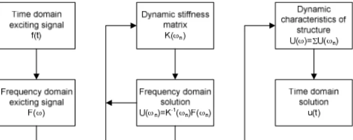
Spectral Finite Element Method (SFEM) has been widely used for modeling wave propagation in mechanical structures (Gopalakrishnan, 2007). This method combines geometric flexibility and competitive advantages of low-order methods, such as finite element method (FEM), with the accuracy and rapid convergence of high order methods (spectral methods). One advantage of SFEM is that the number of elements necessary to model the structure is equal to the number of its sections. Therefore, a spectral element is equivalent to an infinite number of conventional finite elements (Doyle, 1997). Figure 1 shows the diagram to implement SFEM at a particular position on the beam (Ostachowicz, 2008).
Figure 1. SFEM flow diagram for wave propagation in structures.
The spectral response of the structure U(ω) to the excitation signal F(ω) is the sum of the response for each component of the FFT of the time domain excitation signal f(t). For the time domain response of the structure, simply calculate the inverse Fourier transform using the IFFT algorithm.
According to the Bernoulli-Euler beam theory (Doyle, 1997), the displacement u(x,t), as a function of the applied force q, is given by
q t
u A x
u EI
x ∂ =
∂ +
∂ ∂ ∂
∂
2 2
2 2
2 2
ρ , (1)
where EI is the flexural stiffness and ρA is the mass density per unit length. The homogeneous differential equation can be written in spectral form as
0 ˆ
ˆ 4
4 4
= − ∂ ∂
u x
u
β , (2)
with
2 1 2
2
−
=
EI A i A ωη
ρ ω
β , (3)
where η is the structural damping factor per unit volume. The solutions of this equation can be obtained from the following pair of equations:
0 ˆ
ˆ 2
2 2
= − ∂ ∂
u x
u
β and ˆ 2ˆ 0
2 2
= + ∂ ∂
u x
u
β . (4)
The complete solution u(x,t) for a beam of length L can be expressed in the form
( ) ( )
(
)
∑
− + − + − − + − −= Ae ikx Ae kx Ae ikL x Ae kL x ei t
t x
u( , ) 1 2 3 4 ω , (5)
where k is the wave number given by
β =
k .
The first and third terms of Eq. (5) are wave solutions, while the second and fourth are damped vibrations.
For a very slender beam, it may be considered that
( )
( )
x x u x
∂ ∂ =
Φ ˆ . (6)
The vertical displacement and the rotation Φ (x) can be written as
(L x) k(L x)
ik kx ikx
e A e
A e A e A x
uˆ( )= 1 − + 2 − + 3 − − + 4 − −
(L x) k(L x)
ik kx
ikx kA e ikAe kA e
e ikA
x =− − +− − + − − + − −
Φ( ) 1 2 3 4 . (7)
Considering the boundary conditions uˆ
( )
0 =uˆ1, Φ (0)= Φ1,( )
ˆ2ˆL u
u = and Φ (L)= Φ2, the above equations can be written in matrix form as
U H
A= −1 , (8)
where U is the vector of displacements and rotations in points x = 0 and x = L.
For two degrees of freedom, the nodal loads can be written as
( )
2 2( )
x x EI x V ∂ Φ ∂ =
( )
( )
x x EI x M ∂ Φ ∂= . (9)
Whereas the nodal loads at the ends of the beam are given by V(0)=V1, V(L)=V2, M(0)=M1 and M(L)=M2, the nodal loads vector F is given by the following matrix equation:
GA
F=EI . (10)
Substituting Eq. (8) into Eq. (10), F can be rewritten as
U GH
F=EI −1 . (11)
The dynamic stiffness matrix is defined as
1 GH
K=EI − . (12)
Having obtained the dynamic stiffness matrix, the vector of displacements and rotations due to the nodal loads can be calculated by
F K
U= −1 . (13)
For any position, the vertical beam displacement is given by
( ) ( )
[
− − − − − −]
H−1U= ikx kx ikL x kL x
e e
e e x
uˆ( ) . (14)
For a cracked beam, the crack represents a discontinuity of the structure. In this case two elements are required to represent the part of the beam before and after the crack. For a beam of length L and with a crack in position L1, the vertical displacements uˆ1
( )
x and( )
xuˆ2 , and rotations Φ1(x) and Φ2(x) are given by:
(L x) k(L x)
ik kx
ikx Ae Ae Ae
e A x
u = − + − + − 1− + − 1−
4 3
2 1
1( ) ˆ ( ) ( ) 1 4 3 2 1 1 0 , )
( 1 1
L x e kA e ikA e kA e ikA
x ikx kx ikL x kL x
≤ ≤ + + − + − =
Φ − − − − − −
( ) ( ) [ ( )]
( )
[ 1]
8 1 7 1 6 1 5 2( ) ˆ L x L k L x L ik L x k L x ik e A e A e A e A x u + − − + − − + − + − + + + = ( ) ( ) [ ( )] ( )
[ ], 0 .
) ( 1 1 8 1 7 1 6 1 5 2 L L x e kA e ikA e kA e ikA x L x L k L x L ik L x k L x ik − ≤ ≤ + + − + − = Φ + − − + − − + − + − (15)
The nodal loads in the two parts of the beam are
( )
2 12( )
1 x x EI x V ∂ Φ ∂ = ,
( )
( )
x x EI x M ∂ Φ ∂ = 1 1 ,( )
2 22( )
2 x x EI x V ∂ Φ ∂ = ,
( )
( )
x x EI x M ∂ Φ ∂ = 22 . (16)
The boundary conditions for the cracked beam are uˆ1
( )
0 =uˆ1,Φ1(0)=Φ1, uˆ2
( )
0 -uˆ1( )
L1 =-θfV1(L1), Φ2(0)-Φ1(L1)=-θmM1(L1),V1(L1)=V2(0), M1(L1)=M2(0), uˆ2
(
L−L1)
=uˆ2 and Φ2(L-L1)= Φ2. Constants θf and θm are related to crack flexibility for sliding and tearing modes respectively. Details of how to calculate these constants can be found in Tada et al. (2000). Applying the boundary conditions in Eq. (16) and Eq. (15) results in the following matrix equation:c c c H A
U =
c 1 c c H U
A = − . (17)
Whereas the ends of the beam nodal loads are given by V(0)=V1, V(L)=V2, M(0)=M1 and M(L)=M2, the following matrix equation is obtained:
c c c EIG A
F = . (18)
Substituting Eq. (17) into Eq. (18), Fc can be rewritten as
c 1 c c
c G H U
F =EI − . (19)
The dynamic stiffness matrix for cracked beam is defined as
1 c c c G H
K =EI − . (20)
The displacements and rotations vector due to the nodal loads can be obtained by
c 1 c c K F
U = − . (21)
Finally, the vertical displacements for the two sides of the beam are given by
= ) ( ˆ1 x
u [e−ikx e−kx e−ik(L1−x) e−k(L1−x) 0 0 0 0]H c-1Uc
= ) ( ˆ2 x
u
[
0 0 0 0 e−ik(x+L1) e−k(x+L1)e−ik[L−(x+L1)]e−k[L−(x+L1)]
]
Hc-1Uc (22)
Discrete Wavelet Transform
detected through the similarity between its shape in time domain and a waveform known as mother wavelet. The continuous wavelet transform (CWT) of a signal x(t) is given by
( ) ( )
t tdtx s, )=
∫
Ψs*,( τ τ
γ , (23)
where * denotes complex conjugate, s the frequency scale and τ the translation in time. Equation (23) represents the projection of x(t) on an orthonormal base of functions, dilated by s and translated by τ, generated by a function called mother wavelet given by:
( )
− Ψ = Ψ
s t t
s
τ
τ
2 1
, . (24)
This approach fits well to analyze non-stationary signals, because its spectral components vary along time. The propagation of Lamb waves is an example of signal with punctual occurrences. In this case, the wavelet transform is used to extract the wave packages related to the reflections of Lamb waves at beam discontinuities.
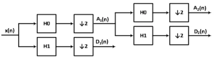
Mallat (1989) presented an efficient method to implement the wavelet transform in discrete time, through multiresolution analysis and digital filter banks. This theory relates the discrete wavelet transform with a filter bank composed of high and low pass quadrature mirrored filters, through which the signal is decomposed into details and approximations. The approximation is obtained as the output of the low pass filter and is related to the smoothed signal. The output of the high pass filter provides the details of the signal, related to transient events contained in the signal. Figure 2 shows the layout of the filter bank, composed of high pass filter (H1) and low pass filter (H0), for two levels of resolution. The symbol ↓2 represents down-sampling or decimation of the filtered signal.
Figure 2. Two level analysis filter bank for DWT.
Each decomposition level of the signal separates the spectral components at frequency bands, which depends on the sampling frequency (fs) of the signal acquired. Figure 3 shows the frequency response of high and low pass ideal filters for 3 level decomposition DWT.
Higher frequency signal components are located at lower level details. Analyzing the signal decomposed into several details provides information that could be hidden in the original signal, probably masked by noise from the measurement system. The subdivision of the signal spectrum in several frequency bands, through the filtering process, is equivalent to the scaling (s) of Eq. (24). On the other hand, the translation (τ) of this equation is obtained by convolution of the signal with the filter coefficients.
One significant advantage of using the DWT approach for signal processing is to design high and low pass filters as digital filters on programmable logic devices, such as modern FPGAs, making it possible to implement the algorithms directly in hardware, which leads to the high performance generally needed in real time signal processing applications (Walker et al. (2003); Nibouche et al. (2002); Chilo et al. (2008)).
Figure 3. Frequency range of High and Low pass filters for 3 levels of decomposition.
Criteria for Selecting the Mother Wavelet Using Shannon's Entropy
Shannon's entropy measures the energy dispersion or randomness within a process. The energy concentration implies entropy lower values. This criterion may be used to choose the best mother wavelet among a group of orthogonal mother wavelet which can be used to transform the signals (Li et al., 2009). Besides to indicate the suitable mother wavelet for signal analysis, the entropy also shows the level of detail that contains information related to reflections of Lamb wave in the structure discontinuities.
For the DWT of a signal x(t), an orthogonal mother wavelet is selected among several possibilities previously chosen for compatibility with the features to be extracted from the signal, for example, Biorthogonals, Coiflets, Daubechies, Symlets, discrete Meyer and others. Whereas cd,i are coefficients of the DWT of x(t), for a mother wavelet chosen arbitrarily the Shannon entropy of detail level d is given by:
∑
=
⋅ =
n
i
i d i d
R c R c d
S 1
2 , 2
, ln )
(
∑∑
= = =D
d n
i i d
c R
1 1 2
, , (25)
0 0.2 0.4 0.6 0.8 1 1.2 1.4 1.6 1.8 2 -2
-1.5 -1 -0.5 0 0.5 1 1.5 2 2.5
time(ms)
A
m
p
lit
u
d
e
(a)
1 3 5 7 9 11 13 15
-3.5 -3 -2.5 -2 -1.5 -1 -0.5 0
detail
S
h
a
n
n
o
n
E
n
tr
o
p
y
db10 dmey sym20
(b)
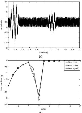
Figure 4. (a) Analyzed Signal; (b) Shannon entropy of DWT coefficients for mother wavelets Db10, discrete Meyer and Symlet 20.
0 0.2 0.4 0.6 0.8 1 1.2 1.4 1.6 1.8 2
-2 -1.5 -1 -0.5 0 0.5 1 1.5 2
time(ms)
A
m
p
lit
u
d
e
Figure 5. Detail level 7 coefficients of DWT with mother wavelet Symlet 20.
Figure 5 shows the level 7 detail’s coefficients obtained by DWT with mother wavelet Symlet 20. It clearly enhances the signal desired attributes. This result shows that the entropy curve of DWT coefficients, for various detail levels, is capable of identifying which level contains the portion of the signal with high concentration of energy.
Hilbert Transform
The Hilbert transform can be used to create an analytical signal from a real signal (Feldman, 2011). Consider x(t) a real signal. The analytic signal xa(t) is calculated as follows:
xa(t) = x(t)+iH{x(t)}. (26)
where H{x(t)} is the Hilbert transform of the real signal. An effective approach to calculate the Hilbert transform is as follows:
1) Calculate the Fourier Transform of the signal; 2) Rotate the phase of the signal obtained at 90°;
3) Return to time domain calculating the inverse Fourier transform.
Writing the analytical signal in polar form, we have:
xa(t) = re-jθ, (27)
where r is the absolute value and θ is the phase of analytical signal. The absolute value of the analytical signal corresponds to signal envelope.
Numerical Results by SFEM Beam Model
The method for detecting faults in structures using Lamb waves and DWT was applied to analyze signals obtained from SFEM model of aluminum beams with length 0.8 m, width 0.031 m and thickness 0.0031 m. A benchmark beam, with no damage, and damaged beams, with a transverse open and non-propagating crack localized at 0.2 m, 0.4 m and 0.6 m with 0.3 crack depth/section height ratio were investigated.
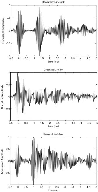
A Hanning windowed five cycle sine tone burst of 14.5 kHz and sampling frequency of approximately 87 kHz was used to generate the Lamb waves. For the sake of getting a more realistic signal, a biased random noise was added to the wave propagation signal obtained from the model, resulting in a 7 dB signal to noise ratio. Figure 6 shows the results obtained by SFEM model with normalized amplitude.
0 0.5 1 1.5 2 2.5 3 3.5 4 4.5 5
-1 -0.5 0 0.5 1
Beam without crack
time (ms)
N
o
rm
a
liz
e
d
A
m
p
lit
u
d
e
0 0.5 1 1.5 2 2.5 3 3.5 4 4.5 5
-1 -0.5 0 0.5 1
Crack at L=0.2m
time (ms)
N
o
rm
a
liz
e
d
A
m
p
lit
u
d
0 0.5 1 1.5 2 2.5 3 3.5 4 4.5 5 -1
-0.5 0 0.5 1
Crack at L=0.4m
time (ms)
N
o
rm
a
liz
e
d
A
m
p
lit
u
d
e
0 0.5 1 1.5 2 2.5 3 3.5 4 4.5 5
-1 -0.5 0 0.5 1
Crack at L=0.6m
time (ms)
N
o
rm
a
liz
e
d
A
m
p
lit
u
d
e
Figure 6. Wave propagation signal obtained by SFEM modeling for beams without and with crack at positions L = 0.2 m, L = 0.4 m and L = 0.6 m.
1 2 3 4 5 6 7 8 9 10
-5 -4.5 -4 -3.5 -3 -2.5 -2 -1.5 -1 -0.5 0
detail
S
h
a
n
n
o
n
E
n
tr
o
p
y
bior6.8 coif3 db40
a)
1 2 3 4 5 6 7 8 9 10
-4.5 -4 -3.5 -3 -2.5 -2 -1.5 -1 -0.5 0
detail
S
h
a
n
n
o
n
E
n
tr
o
p
y
bior6.8 coif3 db40
b)
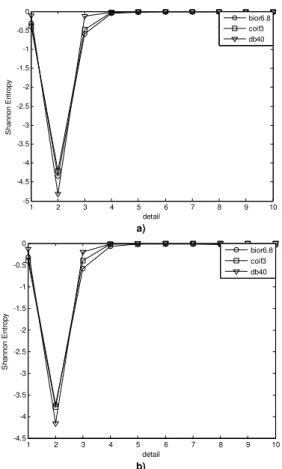
Figure 7. Shannon entropy of the DWT coefficients for beam (a) without crack; (b) with crack at 0.6 m.
0 0.5 1 1.5 2 2.5 3 3.5 4 4.5 5
-1 -0.5 0 0.5 1
Beam without crack
time (ms)
N
o
rm
a
liz
e
d
A
m
p
lit
u
d
e
0 0.5 1 1.5 2 2.5 3 3.5 4 4.5 5
-1 -0.5 0 0.5 1
Crack at L=0.2m
time (ms)
N
o
rm
a
liz
e
d
A
m
p
lit
u
d
e
0 0.5 1 1.5 2 2.5 3 3.5 4 4.5 5
-1 -0.5 0 0.5 1
Crack at L=0.4m
time (ms)
N
o
rm
a
liz
e
d
A
m
p
lit
u
d
e
0 0.5 1 1.5 2 2.5 3 3.5 4 4.5 5
-1 -0.5 0 0.5 1
Crack at L=0.6m
time (ms)
N
o
rm
a
liz
e
d
A
m
p
lit
u
d
e
Figure 8. DWT coefficients of level 2 using the mother wavelet db40 for beams without crack and with crack at positions L = 0.2 m, L = 0.4 m and L = 0.6 m.
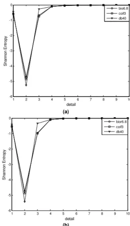
Biortogonal 6.8 (Bior6.8) and Daubechies 40 (db40) were obtained for a maximum level of detail of 10. Figure 7 shows the Shannon entropy of the DWT coefficients for the benchmark beam and the damaged with a crack at 0.6 m. The results for the two beams were similar, i.e., for all cases, the detail curve at level 2 shows the lowest level of entropy for the DWT using the mother wavelet db40. This result is important because it shows that it is possible to determine the optimal mother wavelet and the level of detail from the healthy structure.
The DWT coefficients of second level using the mother wavelet db40 and its envelopes are shown in Figs. 8 and 9 respectively. The curves in Fig. 8 show that after processing the signal, using the DWT, the noise and the bias were extracted. The peaks related to the reflections of Lamb wave at beam discontinuities (boundaries and crack) are much more evident in the processed signal.
The beam length and the crack position are proportional to the time interval between the first two peaks of the signal, corresponding to the excitement and the first reflection of Lamb wave. This is called time of flight (TOF). From Fig. 9, the TOF for the beam without crack was 1.22 ms. This time is equivalent to twice the beam length, because the reflection occurs at the end of the beam. The crack position can be determined by comparing the TOF of the beam without crack with the TOF of the cracked beam, using the following equation:
TOF t
L P
wc
= , (28)
where P is the position of the discontinuity, L is the length of the beam, twc is the time of flight of the benchmark beam and TOF is the time of flight of the beam under test.
Table 1 shows the TOF for beams without and with crack, the estimated crack position and the error between the crack position obtained from the proposed method and its actual position.
Table 1. TOF, crack position estimative and error for numerical model signals.
Crack position Without crack 0.2 m 0.4 m 0.6 m
TOF (ms) 1.22 0.296 0.611 0.888
Estimated crack
position (m) - 0.194 0.401 0.582
Error (%) - 3.00 0.25 3.00
These results prove the effectiveness of the method to detect crack position in beams.
Experimental Validation
To validate the results obtained by the SFEM, measurements were made using two similar aluminum beams of length 0.8 m, width 0.3 m and thickness 0.031 m. The first beam is a regular one and the second presents a cut simulating a crack, localized at 0.6 m or 0.2 m, depending on the side used to excite and measure the Lamb wave reflections. These correspond to the beams modeled, with an exception of the damaged beam with the crack localized at 0.4 m. To excite the beam, a Hanning windowed five cycle sine tone burst of 14.3 kHz was used. The experimental setup consists of two circular buzzers of 2 cm diameter placed side by side at one end of the beam, one to excite the beam and the other to measure the Lamb wave; an Agilent 33120A arbitrary waveform generator; a homemade power and an instrument amplifier; an Instruterm FA-3050 DC power supply; and an Agilent 54622A oscilloscope used to
acquire and to transmit data to a personal computer, where it is processed and analyzed using Matlab®, as illustrated in Fig. 10.
0 0.5 1 1.5 2 2.5 3 3.5 4 4.5 5
0 0.2 0.4 0.6 0.8 1
Beam without crack
time (ms)
N
o
rm
a
liz
e
d
A
m
p
lit
u
d
e
0 0.5 1 1.5 2 2.5 3 3.5 4 4.5 5
0 0.2 0.4 0.6 0.8 1
Crack at L=0.2m
time (ms)
N
o
rm
a
liz
e
d
A
m
p
lit
u
d
e
0 0.5 1 1.5 2 2.5 3 3.5 4 4.5 5
0 0.2 0.4 0.6 0.8 1
Crack at L=0.4m
time (ms)
N
o
rm
a
liz
e
d
A
m
p
lit
u
d
e
0 0.5 1 1.5 2 2.5 3 3.5 4 4.5 5
0 0.2 0.4 0.6 0.8 1
Crack at L=0.6m
time (ms)
N
o
rm
a
liz
e
d
A
m
p
lit
u
d
e
Figure 9. Envelope of level 2 DWT coefficients with mother wavelet db40 for beams without and with crack at positions L = 0.2 m, L = 0.4 m and L = 0.6 m.
Reflexion in boundary Incoming
signal
crack Incoming signal
crack
crack Incoming signal
Figure 10. Experimental setup.
-0.5 0 0.5 1 1.5 2 2.5 3 3.5 4 4.5 5
-1 -0.5 0 0.5 1
Beam without crack
time (ms)
N
o
rm
a
liz
e
d
A
m
p
litu
d
e
-0.5 0 0.5 1 1.5 2 2.5 3 3.5 4 4.5 5
-1 -0.5 0 0.5 1
Crack at L=0.2m
time (ms)
N
o
rm
a
liz
e
d
A
m
p
lit
u
d
e
-0.5 0 0.5 1 1.5 2 2.5 3 3.5 4 4.5 5
-1 -0.5 0 0.5 1
Crack at L=0.6m
time (ms)
N
o
rm
a
liz
e
d
A
m
p
lit
u
d
e
Figure 11. Experimental measurements of beams without and with crack at positions 0.2 m and 0.6 m.
1 2 3 4 5 6 7 8 9 10
-6 -5 -4 -3 -2 -1 0
detail
S
h
a
n
n
o
n
E
n
tr
o
p
y
bio6.8 coif3 db40
(a)
1 2 3 4 5 6 7 8 9 10
-6 -5 -4 -3 -2 -1 0
detail
S
h
a
n
n
o
n
E
n
tr
o
p
y
bior6.8 coif3 db40
(b)
Figure 12. Shannon’s entropy of the DWT coefficients for beam (a) without crack; (b) with crack at 0.6 m.
Figure 11 shows three measured signals for the beams using the above conditions. These signals were measured with a sampling frequency of 100 kHz. It is very difficult to devise the crack position in the damaged beam, and even to be sure of the presence of the crack. The only clear possible conclusion is that the signals obtained from the damaged beam are different from the regular beam.
Figure 13 shows the second level DWT coefficients with the mother wavelet db40 and Fig. 14 their envelope. Comparing the curves of Figs. 11 and 13, the Lamb wave package due to reflections on the crack is much more evident in the processed signal and from the envelopes shown in Fig. 14 the TOF can be measured with high accuracy.
-0.5 0 0.5 1 1.5 2 2.5 3 3.5 4 4.5 5
-1 -0.5 0 0.5 1
Beam without crack
time (ms)
N
o
rm
a
liz
e
d
A
m
p
lit
u
d
e
-0.5 0 0.5 1 1.5 2 2.5 3 3.5 4 4.5 5
-1 -0.5 0 0.5 1
Crack at L=0.2m
time (ms)
N
o
rm
a
liz
e
d
A
m
p
lit
u
d
e
-0.5 0 0.5 1 1.5 2 2.5 3 3.5 4 4.5 5
-1 -0.5 0 0.5 1
Crack at L=0.6m
time (ms)
N
o
rm
a
liz
e
d
A
m
p
lit
u
d
e
Figure 13. DWT coefficients of level 2 using the mother wavelet db40 for beams without and with crack at positions L = 0.2 m and L = 0.6 m.
Table 2. TOF, crack position estimative and error for numerical model signals.
Crack position Without crack 0.2 m 0.6 m
TOF (ms) 1.43 0.36 1.07
Estimated crack
position (m) - 0.201 0.598
Error (%) - 0.5 0.3
Table 2 shows the TOF, the estimated crack position calculated from Eq. (28) and the error between the crack position obtained from the proposed method and its actual position.
The results shown on Table 2 presented less than 1% error for the crack position estimation in these beams. It reinforces the expected good accuracy obtained with the proposed method.
-0.50 0 0.5 1 1.5 2 2.5 3 3.5 4 4.5 5
0.2 0.4 0.6 0.8 1
Beam without crack
time (ms)
N
o
rm
a
liz
e
d
A
m
p
lit
u
d
e
-0.50 0 0.5 1 1.5 2 2.5 3 3.5 4 4.5 5
0.2 0.4 0.6 0.8 1
Crack at L=0.2m
time (ms)
N
o
rm
a
liz
e
d
A
m
p
lit
u
d
e
-0.50 0 0.5 1 1.5 2 2.5 3 3.5 4 4.5 5
0.2 0.4 0.6 0.8 1
Crack at L=0.6m
time (ms)
N
o
rm
a
liz
e
d
A
m
p
lit
u
d
e
Figure 14. Envelope of level 2 DWT coefficients with mother wavelet db40 for beams without and with crack at positions L = 0.2 m and L = 0.6 m.
Conclusions
This work presented a complete method to detect and localize damage in beam type structures based on Lamb waves using the pulse echo configuration and the discrete wavelet transform. Two aluminum beams, one without damage and another with a crack type fault were modeled and simulated using the spectral element method, and an experimental analysis was conducted to confirm the numerical results. The application of DWT and the Hilbert transform on the measured signals improved the accuracy in
Reflexion in boundary Incoming
signal
Crack Incoming signal
Crack Incoming
determining the instants that occurred the signal peaks to obtain the TOF. Furthermore, Shannon’s entropy approach showed the best mother wavelet and the level of decomposition necessary to extract the desirable signal features. Numerical results obtained by SFEM modeling were very close to the measured signals. A damaged beam with the crack at different positions was analyzed to demonstrate the method effectiveness. The results based on the experimental signals showed that, choosing appropriately the mother wavelet and level of detail of the discrete wavelet transform, it is possible to achieve an error less than 1% for the estimation of the crack position. In the current stage of this work, the proposed method was applied to evaluate only beam like structures. Further simulations and experiments with more complex structures like plates and framed panels are needed to confirm the effectiveness of the proposed method.
References
Alleyne, D.N. and Cawley, P., 1992, “The Interaction of Lamb Waves with Defects”, IEEE Transactions on Ultrasonics, Ferroelectrics, and Frequency Control, Vol. 39, pp. 381-397.
Chilo, J. and Lindblad, T., 2008, “Hardware Implementation of 1D Wavelet Transform on an FPGA for Infrasound Signal Classification”, IEEE Transactions on Nuclear Science, Vol. 55, pp. 9-13.
Doyle, J.F., 1997, “Wave Propagation in Structures: a spectral analysis approach”, 2nd ed., New York: Springer.
Feldman, M., 2011, “Hilbert transform in vibration analysis”,
Mechanical Systems and Signal Processing, Vol. 25, pp. 735-802.
Gopalakrishnan, S., Chakraborty, A. and Mahapatra, D.R., 2007, “Spectral Finite Element Method”, London: Springer.
Grondel, S., Paget, C., Delebarre, C. and Assad, J., 2002, “Design of optimal configuration for generating A0 Lamb mode in a composite plate using piezoceramic transducers”, J. Acoust. Soc. Am., Vol. 112, pp. 84-90.
Konstantinidis, G., Wilcox, P.D. and Drinkwater B.W., 2007, “An Investigation into the temperature stability of a guided wave structural health monitoring system using permanently attached sensors”, IEEE Sensors Journal, Vol. 7, pp. 905-912.
Li, F., Meng, G., Kageyama, K., Su, Z. and Ye, L., 2009, “Optimal Mother Wavelet Selection for Lamb Wave Analyses”, Journal of Intelligent Material Systems and Structures, Vol. 00, pp. 1-16.
Lopes Jr., V., Park, G., Cudney, H.H. and Inman, D.J., 2000, “Impedance-Based Structural Health Monitoring with Artificial Neural Networks”, Journal of intelligent Material Systems and Structures, Vol. 11, pp. 206-214.
Lu, Y., Wang, X., Tang, J. and Ding, Y., 2008, “Damage detection using piezoelectric transducers and the Lamb wave approach: II. Robust and quantitative decision making”, Smart Materials And Structures, Vol. 17, pp. 1-13. Mallat, S.G., 1989, “A theory for multiresolution signal decomposition: Thewavelet representation”, IEEE Trans. Pattern. Anal. Machine Intell., Vol. 2, pp. 674-693.
Mallet, L., Lee, B.C., Staszewski, W.J. and Scarpa, F., 2004, “Structural health monitoring using scanning laser vibrometry: II. Lamb waves for damage detection”, Smart Materials and Structures, Vol. 13, pp. 261-269.
Nibouche, M. and Nibouche, O., 2002, “Design and implementation of a wavelet block for signal processing applications”, 9th International Conference on Electronics, Circuits and Systems, Vol. 3, pp. 867- 870.
Ostachowicz, W.M., 2008, “Damage detection of structures using spectral finite element method”, Computer & Structures, Vol. 86, pp. 454-462.
Park, G., Sohn, H., Farrar, C.R. and Inman, D.J., 2003, “Overview of piezoelectric impedance-based health monitoring and path forward”, The Shock and Vibration Digest, Vol. 35, pp. 451-463.
Sirohi, J., Chopra, I., 2000, “Fundamental understanding of piezoelectric strain sensors”, Journal of Intelligent Material Systems and Structures, 11, pp. 246-257.
Su, Z. and Ye, L., 2009, “Identification of Damage using Lamb Waves – From fundamental to applications”, Lecture notes in applied and computational mechanics, Vol. 48, 1st Edition, London, Springer.
Sun, Z. and Chang, C.C., 2002, “Structural Damage Assessment Based on Wavelet Packet Transform”, Journal of Structural Engineering, pp. 1354-1361. Tada, H., Paris, P.C. and Irwin, G.R., 2000, “The stress analysis of cracks handbook”, 3rd ed., New York: The American Society of Mechanical Engineers.
Walker, S.L., Foo, S.Y. and Petrone, J., 2003, “On the Performance of a Hardware Implementation of the Wavelet Transform”, Proceedings of the 35th Southeastern Symposium on System Theory, Vol. 16, pp. 397- 399.
Wang, Q. and Deng, X., 1999, “Damage detection with spatial wavelets”, International Journal of Solids and Structures”, Vol. 36, pp. 3443-3468.
Wang, X., Lu, Y. and Tang, J., 2008, “Damage detection using piezoelectric transducers and the Lamb wave approach: I. System Analysis”,