A Work Project, presented as part of the requirements for the Award of a Masters Degree in Economics from the NOVA – School of Business and Economics.
Productivity Gains from Migration: An Analysis of Cape Verdean
Return Migrants
1Guilherme Rodrigues, nº541
A Project carried out under the supervision of: Professor Cátia Batista
January 7, 2015
2
Abstract
Are return migrants more productive than non-migrants? If so, is it a causal effect or simply self-selection? Existing literature has not reached a consensus on the role of return migration for origin countries. To answer these research questions, an empirical analysis was performed based on household data collected in Cape Verde.
One of the most common identification problems in the migration literature is the presence of migrant self-selection. In order to disentangle potential selection bias, we use instrumental variable estimation using variation provided by unemployment rates in migrant destination countries, which is compared with OLS and Nearest Neighbor Matching (NNM) methods.
The results using the instrumental variable approach provide evidence of labour income gains due to return migration, while OLS underestimates the coefficient of interest. This bias points towards negative self-selection of return migrants on unobserved characteristics, although the different estimates cannot be distinguished statistically. Interestingly, migration duration and occupational changes after migration do not seem to influence post-migration income. There is weak evidence that return migrants from the United States have higher income gains caused by migration than the ones who returned from Portugal.
Keywords: return migration; productivity; labour income gains; self-selection; Cape Verde
1. Introduction
3
countries, representing 10.8% of total population in these countries2. According to the World Bank, between 1990 and 2013 the average annual flow of migrants was around 3.3 Million, around one third had a developing country as destination.
When analyzing the benefits and costs of migration, one should precisely define the target of this analysis: it may be migrants individually; the whole destination society or even an origin country’s society. This Work Project will follow the literature in measuring individual economic effects of return migration in the country of origin (Cape Verde). The aim of this work is to identity whether return migrants gain productive skills while abroad.
During the last decades, the debate on the impact of migration on the economic development of countries of origin has been lively. On the one hand, some authors highlight the disadvantages of migration summarized by “brain drain” arguments. These can be described as a society’s losses due to the emigration of skilled individuals3, which cause a direct human capital loss, particularly in critical sectors such as education, health and public service, that has an effect on national output, both directly and through human capital externalities. One can also consider other indirect channels such as the reduction of the quality of institutions through diminished demand for political accountability or a reduced supply and competition for public services4.
On the other hand, recent literature describes potential benefits of migration specifically to the countries of migrant origin. One example is the “brain gain” theory -arguing that migration outflows may cause human capital gains for the non-migrant
2 United Nations Department of Economics and Social Affairs, Population Division: Population Facts, September 2013.
3 Scott and Gruber (1966) and Bhagwati and Hamada (1974) were the main proponents of “brain drain” arguments.
4
population by increasing the expectations of future migration (even if it never happens)5. Additional research examines the potential benefits of migration on political participation and the quality of institutions’ in migration origin countries6. Migration may also lead to an increase in business creation/productive investment due to increased skills and liquidity provided by migrant savings and remittances7, and to contribute positively to international trade and foreign direct investment8.
The focus of our work is to measure the potential benefits of migration for individual skills when they are back to the country of origin. It is found that return migrants have labour income gains due to migration, after accounting for self-selection patterns, both in terms of observable and unobservable characteristics. This result contrasts to that of Lacuesta (2008), who uses a sample of Mexican migrants to examine the same research question, but fails to reach the same conclusions, but is according to Gibson and McKenzie (2010) using a sample of Tongan return migrants.
The structure of the Work Project is the following: Section 2 summarizes the most relevant literature. Section 3 gives the background for Cape Verde. Section 4 describes the household survey used in the empirical analysis. In section 5, the econometric models are discussed. The empirical results are presented in section 6. Finally, in Section 7, the main findings and policy implications are offered. Annex 1 presents all tables with the empirical results; Annex 2 describes Borjas and Bratsberg (1996)’s theoretical model; and Annex 3 presents an English version of the survey conducted.
5The “brain gain” theory was developed by Mountford (1997), Stark et al. (1997, 1998) and Vidal (1998).
Empirically, the theory was tested at the micro level by Batista et al. (2012), and across countries and over time by Faini (2006); Ozden and Schiff (2006) and Beine et al. (2007, 2008).
6 Batista and Vicente (2011).
7 Dustmann and Kirchkamp (2003), Mesnard and Ravallion (2006), Yang (2008), and Batista et al. (2014). 8 Gould (1994), Rauch and Trindade (2002), Kugler and Rapoport (2007), Iranzo and Peri (2009) and
5
2. Literature Review
The approach of this paper is to examine the wage differential between non-migrants and return non-migrants, which is taken as a proxy for the corresponding productivity differential. In addition, the nature behind the gap will be studied. We begin by summarizing and discussing the relevant literature for this examination.
Borjas and Bratsberg (1996) developed an economic model to explain migration9. Their starting point is Roy’s Selection Model (1951). Their main contribution is the study of migrant’s selection patterns relative to the distribution of skills/income in the origin and destination countries. The authors consider migration as a decision variable in maximizing life-cycle earnings: individuals decide whether they migrate or not taking into account the costs and benefits of migration over their lifecycle. This model makes two predictions regarding the phenomenon of return migration: first, individuals obtain human capital by migrating that will reflect higher productivity and wages at home. If productivity gains are high enough, returning to the home country may be the optimal scenario to maximize individual welfare. Second, return may be a decision caused by uncertainty about the wages prior migration. When an individual decides to migrate basing his decision on an expected wage higher than the real one, returning may be optimal10.
Borjas and Bratsberg (1996) also analyze migrant characteristics and self-selection patterns. According to them, the monetary return on unobserved characteristics will determine who migrates. When the return on unobserved characteristics is higher abroad, migrants will be highly skilled relative to non-migrants (positive self-selection on unobserved characteristics). The opposite will happen if the return on unobserved
9 Model developed in Annex 2.
6
characteristics is lower abroad. In any event, return migrants will be in the middle of the skill distribution of non-return migrants and stayers11. Borjas (1987) finds negative selection of the observed characteristics based on the idea behind the Borjas and Bratsberg (1996) model.
There is no consensus in the literature on migrant selection in terms of observed characteristics: opposing to Borjas (1987), Chiswick (1978) finds negative selection12. Recent work has focused on examining patterns of migrant self-selection on unobserved characteristics13. Akee (2010) studied American immigrants from Micronesia. In this setting, free mobility between these countries eliminated destination country screening that would potentially cause a selection bias. Akee (2010) finds that unobserved characteristics are positively related with migrant’s self-selection14 when matching pre-migration ages. The author also uses tropical typhoons and household assets damaged by them as instrumental variables finding strong evidence of positive self-selection based on unobserved characteristics with the previous method.
McKenzie et al. (2010) use an experimental measure to examine income gains from migration and analyze self-selection on Tongan migrants in New Zealand. New Zealand has an annual quota for Tongans to reside there permanently. As the number of vacancies is lower than the demand for visas, there is a lottery to randomly choose who migrates across applicants. In this specific setup, the authors are able to quantify income gains from migration by comparing ballot’s winners and losers, who are supposed to have similar unobserved characteristics before migration (e.g. motivation). From comparing non-applicants with applicants, there is evidence towards positive self-selection on the unobservable characteristics by migrants/applicants. The authors also compare the
11 For details on this derivation, please refer to annex.
12 Both authors have studied immigrants in the same country (the United States). 13 Such as courage, risk aversion, ability, motivation, etc.
7
previous experimental measure with non-experimental measures15. Estimation using Instrumental Variable seems to be the only non-experimental method which does not overestimate results16.
Some specific research has been done on the impact of return migrants in their origin countries. Lacuesta (2006) has studied potential productivity gains from migration and self-selection of Mexicans who migrate to the United States. The author found a wage premium of 7% for migrants staying abroad more than three months but he argues that there is no evidence of productivity gains caused by living abroad. The wage gaps between migrants and non-migrants are just a result of pre-migration productivity differences. To support the idea of positive self-selection in terms of unobservable characteristics, the author compares non-migrants with migrants who have been abroad for shorter periods than one year17. Short-term migrants have higher wages than non-migrants, which seems to be explained by pre-migration characteristics. However, the author warns that previous differences might be a signaling instrument of individual unobserved characteristics.
Gibson and McKenzie (2010) have an important contribution measuring human capital gains on return migrants from Tonga and Vanuatu. They study a seasonal program in New Zealand which is focused on unskilled workers. The authors conclude that migrants have human capital gains while they are abroad18.
Batista et al. (2014) evaluate how entrepreneurial return migrants are by comparing them with non-migrants in Mozambique. The authors find a way of tackling
15
McKenzie et al. (2010): Non-experimental measures used are first differences, OLS, difference-in-differences, matching, and instrumental variables.
8
the self-selection bias, unlike previous research19. To account for unobservable self-selection bias at both the initial migration stage, and at the return migration stage, the authors use variation provided by the independence and civil wars in Mozambique, GDP variation in Mozambique relative to the main destination countries, as well as social unrest factors such as violence in the destination countries. It is found that having a return migrant in the household increases the probability of business ownership by 22-27%.20 It is concluded that overall negative self-selection partially hides the effect of return migration on entrepreneurship.
3. Cape Verde: General Description21
Cape Verde is a country with a total population of 491.875 individuals22 distributed over nine islands. In 1975, the country became independent from Portugal and in 1991 democracy was established. In 2012, GDP per capita (purchasing power parity adjusted) was approximately 6422 dollars and the unemployment rate was 7.6%.
As consequence of large migration outflows, Cape Verde is a country characterized by high levels of remittances. In the period 2000-2012 annual remittances represented on average 10.6% of total GDP which corresponds to more than one third of the value of exports for the same period. According to Batista et al. (2011), official statistics may undervalue total migrant remittances because they do not consider informal channels.
19 Mesnard (2004); and Mesnard and Ravallion (2006) had a contribution of the importance of emigrants in creating new businesses in Tunisia through overcoming liquidity/credit constraints. Dustmann and Kirchkamp (2002) study the optimal migration duration and occupational change after returning of former Turkish emigrants from Germany who returned home in 1984.
20 Simple estimates which do not tackle self-selection properly measure an increase of business ownership between 9% and 12%.
21 In the following section, data come from the World Bank if not stated otherwise.
9
Historically, migration plays an important role in Cape Verdean society. Mass migration started due to famines and droughts23. In recent years, net annual migration in relation to total population was 6.5% in 2007 and 3.5% in 2012. Estimates from 2013,24 show that around 170,000 Cape Verdeans are living abroad25. The most typical migration destinations are Portugal and the United States26. As most migrants decide to migrate to developed countries with higher productivity levels, it is interesting to study possible productivity gains caused by assimilation of migrants in these countries.
4. Data
4.1 Overview
The empirical analysis will be based on representative household survey data27 collected between December 2005 and March 2006 by the CSAE28 at the Oxford University. The data collection was conducted in 30 out of the 561 existing census areas in Cape Verde in four different islands: Santiago, Fogo, São Vicente and Santo Antão.
The sample is composed of 1066 resident households chosen to ensure its representativeness of Cape Verde. Overall, there is information on 7242 individuals of which 179 are return migrants.
4.2 Descriptive Statistics
In order to check the representativeness of the data collected, comparisons with official statistics were done, especially of migration specific data.
When comparing migrants’ outflows between 2000 and 2005 with the official data, the following can be observed: migration outflows represented 2.02% of the average
23 Batista et al. (2009).
24 Migration Policy Institute from United Nations, Department Economic and Social Affairs (2013).
25
10
annual population for this period according to the INE data, while in our sample the number of migration outflows represented 3.96% of the total sample for the same period. The weight of return migrants in the total number of migrants is around 19.5% in our sample comparing with 25% for the period between 1995 and 2000 (Census 2000). The two most common destinations of Cape Verdean migration are Portugal and the United States, representing respectively 55% and 20% of migration flows in the survey, which compares with 54% and 19% in the period 1995-200029.
The sample’s gender composition is characterized by 51.84% of females while the official data shows a share of 50.5%30 of females in the Cape Verdean population (2010). The percentage of male migrants in the sample is the same as the official statistics for the period 1995-2000, representing 51.4% of the total number of migrants.
In 2010, the population above 65 years old represented 6.4% of total population while it accounts for 5.7% of the whole project’s sample. Individuals aged between 15-64 years old represent 65.9% of the sample, four percentage points more than its weight in Cape Verdean total population in 2010. The weight of individuals living in urban areas is 61.8% for both the sample and the official 2010 census data.31
5. Econometric Framework and Empirical Strategy
Initially, an estimation model analysis will be done taking into consideration potential estimation problems. From this, it will be possible to propose an efficient econometric estimation method.
We are interested in comparing the labor income outcomes of return migrants with those of non-migrants. However, as long as these two outcomes are exclusive, it is not possible to compare them in a fixed point in time for the same individual - at time t, we
29 Census (2000).
11
cannot compare the current income of a return migrant with the current income he/she would have earned if he had not migrated.
Current labour income of a return migrant is composed of two components: the counterfactual labour income that he/she would earn if he/she had not decided to migrate, plus the extra income earned because of migration. Supposing that the counterfactual non-migrant labour income would be the same for migrant and non-migrant groups, the causal effect of migration would be the difference between the earnings of two individuals with the same observable characteristics32. However, it is unlikely that this assumption is valid. Generally, it can be concluded that differences between migrants and non-migrants are not simply the causal effect of migration due to individual self-selection. Self-selection can be caused by observable and unobservable characteristics.
Studying self-selection is therefore important not only to avoid a biased empirical analysis, the nature of selection is in itself an extremely important research question to understand migrations flows.
5.1 Ordinary Least Square (OLS) Estimation
As a starting point, the following Ordinary Least Square Estimation model will be analyzed:
(1) ln(Yi) = αi + Riθ + Xiβ + εi
Where ln(Yi) represents the logarithm of individual i’s monthly labor income in
equation 1, which serves as a proxy of labour productivity; Ri is a binary variable that
states whether individual i is a return migrant; and Xi is a vector of individual
12
characteristics of individual i such as age, gender and personal occupation, that may affect labor income.
The coefficient of interest (𝜃) will identify the causal effect of return migration on labor income if the following condition is satisfied: the error term of the equation (εi) is
not correlated with the decision of return migration (Ri). One possibility would be
incorporating all variables that influence the decision of migration as controls to get rid of endogeneity. However, it is hard to believe that one can measure and incorporate in the regression all factors influencing migration decisions. As long as there are unobserved characteristics which influence the outcome of interest differently across groups of migrants and non-migrants, equation 1 will suffer from a selection bias leading to a biased causal effect coefficient. This biased coefficient from equation 1 will be extremely useful to compare with an unbiased coefficient33 and understand the nature of self-selection.
5.2. Nearest Neighbor Matching (NNM) Estimation
Nearest Neighbor Matching estimation compares individuals from different groups within the sample: return migrants and non-migrants. The idea behind the method is to set a certain number of variables to be similar or equal among groups (e.g. age, gender). Then, the impact of return migration on productivity can be estimated by getting the differences between treated and non-treated individuals. Matching is not necessarily done on a one-to-one comparison, one can set n-to-n comparison34 estimation. The treatment coefficient is calculated by subtracting non-migrants’ income average from migrants’ income average. As the OLS estimation, this method only generates unbiased estimators if there is no selection bias.
13
Compared to OLS, Nearest Neighbor Matching is less restrictive in terms of the observable characteristics (it just compares “comparable” individuals) and it does not need to be a linear functional form as in OLS.
In section 6, results of nearest neighbor matching estimation will be presented together with its results.
5.3 Instrumental Variable (IV) Estimation
5.3.1 Methodology
In order to overcome any selection bias, instrumental variable estimation was performed to identify the causal effect of return migration on labor income.
(2) ln(Yi) = αi + Riθiv + Xiβ + εi
(3)Ri = ϕi + Xiδ + IV𝜑+ ∈i
An instrument is a variable or a set of variables (Zi) used as a proxy of the return
migration variable of interest (Ri) that is not correlated with the dependent variable, Yi. It
can be decomposed in two components: the part correlated with εi and the one which is
not correlated. When isolating the uncorrelated component, it is possible to estimate an unbiased coefficient for the regressor of interest, Ri . A proper instrument must obey the
following conditions:
(4) cov(zi
,
Ri) ≠ 0(5) cov(zi
,
εi) = 0Indeed, the instrumental variable must be correlated with the instrumented variable (Ri) and it must be exogenous, meaning that the error term in the explanatory
14
correlated with the dependent variable only through the instrumented variable; it cannot be related with εrj (unobservable characteristics such as ability, courage, etc).
The instrumental variable estimation process we follow is Two-Stage Least Squares (2SLS) and is based on equations 2 and 3. Equation 3 is the first stage of the estimation (OLS procedure) where the instrumented variable (Ri) is estimated based on
the instruments selected (IV) and other controls. Then, predicted values of R (𝑅̂) of the first stage equation are computed.
(6) 𝑅i =∅ + 𝑋
̂
i𝛿 + 𝐼𝑉𝜑Then it is possible to estimate the model presented in equation 2 using OLS where ln(Yi) is regressed on the predicted values of R (𝑅̂) from the first stage equation, which
provides an unbiased coefficient on return migration (𝜃𝑖𝑣). Note that standard errors need to be adjusted appropriately to be valid.
5.3.2. Choice of Instrumental Variables
In order to conduct the 2SLS estimation, it is necessary to find a variable that is not directly related with actual income from labour and is related with the probability of migrating and return. Based on the work made by Batista et al. (2009) and Batista et al. (2012) a set of macroeconomic variables was chosen to be instruments. One of the ways of instrumenting migration decisions was through unemployment rates and nominal GDP per capita in the main destination countries35. Batista et al. (2012) use changes in GDP per capita36 in Mozambique and in the destination countries. The instruments selected in
35
15
this study are unemployment rates and the percentage change of the unemployment rates in comparison with the previous year for the main destination countries37.
The reasoning behind the selection of this instrument is the following: on one hand, unemployment rates and their variations in destination countries are related with the probability of a migrant to get/keep a job abroad which may influence the decision of migrating and returning. On the other hand, unemployment rates abroad do not seem to be directly related with current labour income. The instrument is composed by four variables per country. For the returning migrants these are: unemployment rates in the year of migration and in the year of return and the yearly variation (percentage) of the unemployment for the same years. For the non-migrants: unemployment rate and its yearly variation for the years in which the individual has the average age of migrating and the average age of returning in the sample38. This method can be interpreted as the age in which a non-migrant was more likely to migrate. This approach is made to create a variable that corrects from self-selection in both migration and return stages.
5.4. Testing Instrument’s Quality
After choosing an instrument, one should know whether it is a valid instrument. It is necessary to test the conditions presented in equations 4 and 5.
5.4.1. Instrument Exogeneity: Hansen Test
The model is characterized by an overidentified system (several instruments for one instrumented variable), which allows testing for instrument exogeneity. The most appropriate test for our model is the Hansen Test, which is a derivation of the Sargan Test39. This test is built by computing the residuals from the instrumental variable’s second stage and regressing them on all exogenous variables. The null hypothesis states
37 The countries are Portugal, United States, Spain, Switzerland, Italy, Luxembourg and Netherlands. 38 The average age of migration is 36 years old and the age of return is 42.
16
that the instrument is correlated with the residuals (endogenous coefficient)40. To consider an instrument exogenous, it is necessary to reject the previous hypothesis. The criteria adopted to reject the null will be a p-value above 0.15 which is commonly used in the literature.
5.4.2. Strength of the Instrument: Stock and Yogo41 Procedure
An exogenous instrument is a necessary but not a sufficient condition to have a valid instrument. It needs to be a strong instrument, meaning that the correlation with the endogenous variable must hold. The test used to validate this condition is the one proposed by Stock and Yogo (2005). It is based on Cragg-Donald (1993)42 test made for a single endogenous variable which is simply an F-Statistic of the first stage regression (equation 3). The null hypothesis states that the instrument is weak and the test statistic is an F-Statistic based Kleibergen-Paap Wald Statistic43. In order to reject the null hypothesis, Kleibergen-Paap F-Test statistic above 10 is required according to most of the literature.
6. Estimation Results44
6.1. Estimation from Baseline Models
In this section, main empirical results from the models specified previously will be presented. All individuals younger than 18 years old were excluded from the models. The previous restriction tries to avoid inclusion of individuals who are not labour force. Then, income gains from migration are estimated using three different sets of controls45.
40 The test-statistics follow a chi-square distribution with k-m degrees of freedom (k is the number of excluded instruments and m, the number of endogenous variables.
41 Stock, and Yogo (2005). “Testing for Weak Instruments in Linear IV Regression”, in
Identification and Inference for Econometric Models: Essays in Honor of Thomas Rothenberg, ed. D. Andrews and J. Stock, 80-108. Cambridge University Press.
42 Cragg-Donald Wald Statistics are not valid in this case because we are in the presence of cluster-robust statistics.
43 Chi-Square distribuition following (k-m+1) degrees of freedom where k is the number of excluded instruments and m the number of endogenous regressors.
44
All estimations presented in Annex 1.
17
The estimation methods were OLS, Nearest Neighbor Matching46 and Instrumental Variable. With the exception of the Instrumental Variable procedure, all models will have 1011 observations where 59 of them are return migrants47.
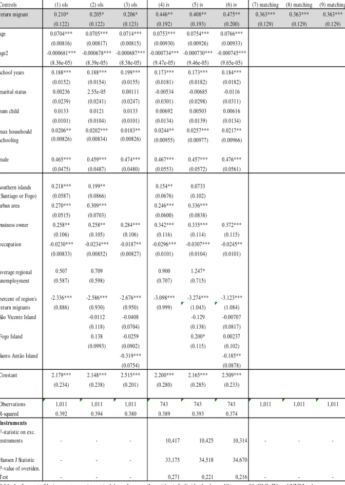
In the first approach made (Table 1), the effect of return migration on labour income is 20-21% in the OLS models compared to 41-48% in the models using instruments. OLS coefficients are statistically significant at a 10% level while the ones using instrumental variable are significant at a lower level (5%).
The difference among coefficients suggest that migrants select themselves negatively in terms of unobserved characteristics. Selection of the unobservable will be tested later in this section.
It is relevant to highlight that both models show that variables as age, schooling, having a business and being male cause a positive impact on labour impact48
Matching coefficients have a magnitude of 0.36 and are highly significant49. Coefficients’ magnitudes are between the ones estimated by the other two methods.
6.2. Inclusion of Migration Specifics
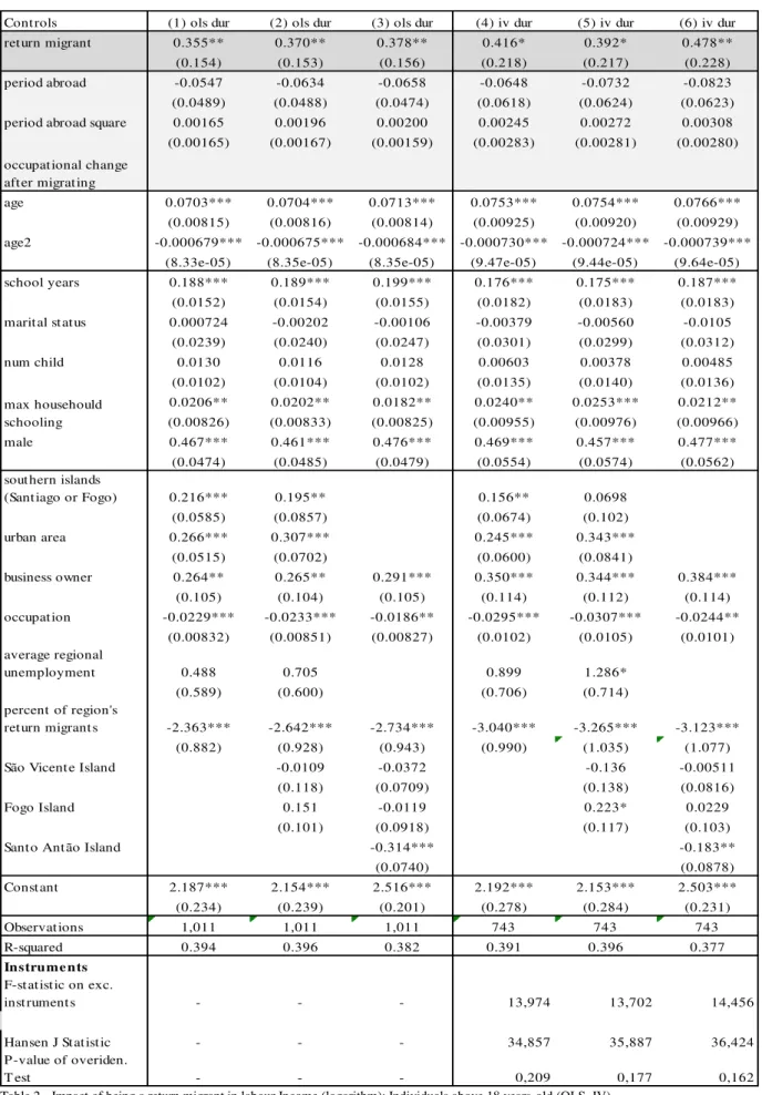
After having shown that migration seems to have an impact on productive skills, it will be interesting to study: i) if this is a time cumulative effect; ii) the channels behind this effect. To answer to these questions, further estimation was done including post migration controls50: migration’s duration (years) and job changes after migration51. Based on the models presented previously, it was build a model to test if destination country is relevant to determine productive skills gains (Table 4).
46 Forcing exact match for age education and gender. The number of matches per observation will be at least 10.
47 In this method we have 743 observations with 59 migrants. 48 Significant at least at a 5% level for all models in Table 1. 49 Significant at a 1% level.
18
Nearest neighbor matching procedure is not used in this analysis because when including post-migration characteristics, it is not possible to compare both groups properly.
When adding the controls for migration’s duration (Table 2), one cannot reject the hypothesis that an extra year spent abroad by a return migrant does not affect labour income52. However, return migration by itself partially explains the outcome of interest. OLS coefficients are significant at a 5% level and IV estimation is significant at 5% or 10% level depending on the model (highest p-value equals 7%). Instrumental Variable coefficients are still higher than the ones estimated by OLS but the gap between the two estimation methods is narrower (OLS of 36-38% against IV of 39-48%). It seems that productive skills gained abroad mostly depend on the event of migrating and not on the total time spent abroad.
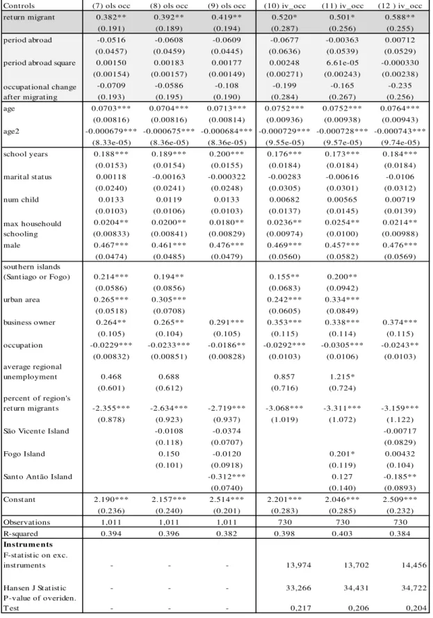
To study the impact of changes between prior and post migration jobs, abinary53 control was included to the model presented above. Table 3 shows that the previous effect does not explain income gains. Return migration itself still causes an increase in labour income54. Opposing to the models without job changes, the gap between the OLS and instrumental variable estimation is relatively wide55 which may result from selection of the unobserved characteristics.
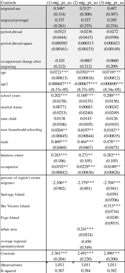
When evaluating the role of destination countries in income gains, no instrument was found that would explain the decision of choosing a specific destination country. Most of migrants decide to go to the United States or Portugal56, so the impact of
52 Both variables are not individuals or jointly significant at a 10% level in any model regressed. 53 Equals 1 if person has a different type of job, zero otherwise.
54 Always significant at a 5% level. With the exception of one of the models with instruments, it is significant at a 1% level.
19
migrating to these specific countries was estimated in three different sets of controls (Table 4). Post-migration controls like duration and occupational change are also included in the model to avoid endogeneity when measuring the role of the destination country itself.
Migrating to the United States seems to contribute more to labour income gains compared to Portugal (49-54% instead of 29-34%). The United States’ coefficient is significant at a 10% level for two of the models while the one of Portugal is never significant at the previous significance level. On one hand, both coefficients together are significant at a 10% level. The results should be seen in a very careful way due to the fact that no valid instrument is used to tackle potential endogeneity.
On the other hand, there is no evidence that migrating to the United States causes a higher increase in labour income (after returning) than Portugal.
For all models estimated with post-migration controls, the main conclusions about socio-economic controls are similar to the ones presented previously.
6.3. Self-Selection of the Unobserved Characteristics
It was discussed through the project that individuals that decide to migrate and return may have some specific characteristics which are non-observable. The use of valid instruments and their comparison with regular estimators should give us an answer on that.
20
compares the OLS and IV equivalent coefficients57. In case of negative self-selection, the null hypothesis should be rejected which implies that coefficients are equal.
When dividing the models by post-migration controls58, there is only some weak evidence of negative self-selection of the unobserved characteristics in the group without post-migration controls. In the group with no post-migration controls, the p-value for the selection test is approximately 12.6% and 16.8% for two of the models (Table 6). For all of the other models, the null is rejected for a confidence interval above 20%. In most of the cases, the OLS underestimation is not enough to prove the presence of negative self-selection of the unobserved characteristics.
6.4. Robustness Tests
Until this point, all conclusions were based on the idea that the models are robust. It is however necessary to prove this. Two questions will be addressed in this section: i)
are the instruments selected valid? ii) Are the models representative for the whole sample or is there any problem caused by the non-included individuals who do not report their wage?
6.4.1. Instrumental Variables Validity
In section 5, the criteria behind instrumental variable selection was discussed based on economic theory and literature examples. Table 5 summarizes all tests59 necessary for every regression done with an instrument.
According to the criteria set previously, instruments seem to be valid. First, Kleibergen-Paap Wald’s F-statistic is above 10 in all cases which means that the instrument is correlated with the instrumented variable. It should be taken into account
57 Both models with the same controls.
58 The three following groups: one with no post-migration controls; other with duration as post-migration control and another with all post-migration controls (duration and job change).
21
that in the models without post-migration characteristics, F-statistics are slightly above 10 (between 10.3 and 10.4). Moreover, there is no evidence that the selected instruments suffer from endogeneity, having a Hansen p-value above 0.15 for all models considered. There is also no evidence that the instruments estimated do not follow the two fundamental conditions60 to form a proper instrument.
6.4.2. Heckman Correction Procedure
In survey data, it is common to have missing values of certain variables which may be a result of voluntary omission or unawareness. In the project’s sample, income from labour is the variable where omissions occur more frequently and this may influence the results. To describe the potential problem, only 59 out of 167 return migrants reported their labour income. As long as omissions may be related with specific characteristics, we cannot be sure that our sub-sample is representative. The Heckit model61 was built to consider individuals with missing values62 in certain variables, tackling self-selection.
The tests done were a comparison between the impact of return migration on labour income in the Heckit model and the OLS model using the same controls. If we reject the hypothesis that both coefficients are different, the OLS model will be considered representative. As long as OLS is considered representative, the models that have instruments will also be considered representative. There is no evidence that OLS and Two-Stages Least Squares models are not representative of the sample, since the null hypothesis is never rejected for a confidence interval below 40% (Table 7).
No model for correcting excess of zeros was done (e.g. Double Hurdle Model) due to the fact there are few individuals reporting their labour income as zero.
60 Exogenous and correlated with the instrumented variable. 61 Also known as Heckman Correction Model.
62 Two stages method: the first stage is to run a model that predicts labour income (in this case) based on other variables; the second stage predicts the impact of each control on labour income (previous
22
7. Conclusions
Studying costs and benefits of migration is extremely important in a country like Cape Verde given its socio-demographic characteristics. This project tried to answer whether migrating and returning to the origin country improves income from labour. This was done by using instrumental variables to tackle self-selection problems. The project shows that return migrants have a wage premium caused by migration between 40.8 and 58.8% when using instrumental variable estimation which is considered the most proper method between the ones chosen by the author. The selected instruments were based on macroeconomic shocks (destination countries’ unemployment rates and their annual variations) and was proved to be valid: correlated with the decision of migration and exogenous (not correlated with variables as courage or risk preferences).
OLS and Nearest Neighbor Matching seem to undervalue the impact of migration on labour income when comparing with instrumental variable estimation. However, there is no evidence that these methods are statistically different between each other; one cannot guarantee the presence of negative self-selection of the unobservable characteristics.
While analyzing the mechanisms behind the impact stated above, there is no evidence that migration’s duration and occupational changes after migrating have a direct impact on labour income. There is scarce evidence that migrating to the United States has a higher impact on home labour income when comparing with migrating to Portugal. Socio-demographic characteristics such as age, gender and schooling seem to influence labour income as expected.
23
In terms of policy implications, central and local authorities should try to reduce costs of returning to the country of origin in order to improve their stock of human capital. First, reducing the cost of return can be done indirectly by reducing fees for cash flows from abroad (e.g. savings of migration). Second, reducing bureaucracy such as recognizing qualifications attained abroad. These policies may incentive migrants to return.
24
References
Akee, R. (2010): “Who’s Leaving? Deciphering Immigrant Self-Selection From a Developing Country," Economic Development and Cultural Change, 58, 323-344. Batista, Catia & Pedro C. Vicente. (2011): “Do Migrants Improve Governance at Home? Evidence from a Voting Experiment," World Bank Economic Review, World Bank Group, vol. 25(1), pages 77-104, May.
Batista, C., A. Lacuesta, and P. C. Vicente (2012): “Testing the `Brain Gain'
Hypothesis: Micro Evidence from Cape Verde," Journal of Development Economics. Batista, Catia & McIndoe Calder, Tara & Vicente, Pedro C., (2014): “Return Migration, Self-Selection and Entrepreneurship in Mozambique,”, “IZA Discussion Papers 8195, Institute for the Study of Labor (IZA)”
Beine, Michel, Cecily Defoort, and Frederic Docquier (2007): “A Panel Data Analysis of The Brain Gain”, Mimeo, Université Catholique de Louvain.
Beine, Michel, Frederic Docquier, and Hillel Rapoport (2008). “Brain drain and LDCs’ growth: winners and losers”, Economic Journal, 118:631-652.
Borjas, G. J. (1987): “Self-Selection and the Earnings of Immigrants", American Economic Review, 77, 531-53.
Borjas, George J., and Bernt Bratsberg. (1996): “Who Leaves? The Outmigration of the Foreign-Born”, Rev. Econ. and Statistics. 78 (February): 165–76.
Chiquiar, D. and G. Hanson (2005): “International Migration, Self- Selection, and the Distribution of Wages: Evidence from Mexico and the United States", Journal of Political Economy, 113, 239-281.
Chiswick, B. (1978): “The Effect of Americanization on the Earnings of Foreign-born Men”, The Journal of Political Economy, Vol. 86, No. 5, pp. 897-921.
Faini, Riccardo (2006): “Remittances and the Brain Drain”, IZA Discussion Paper
2155.
Gibson, J. and D. McKenzie (2010): “The Development Impact of a Best Practice Seasonal Worker Policy", Policy Research Working Paper WPS5488, World Bank. Gould, D. (1994): “Immigrant Links to the Home Country: Empirical Implications for U.S. Bilateral Trade Flows", Review of Economics and Statistics, Vol.76, No.2, pp.302-316.
Heckman, James J. (1979): “Sample Selection Bias as a Specification Error.”, Econometrica 47(1): 153-161.
Instituto Nacional de Estatistica (2000): Recenseamento Geral da População e da Habitação. Cidade da Praia, Cabo Verde: INE.
Instituto Nacional de Estatistica (2010): Recenseamento Geral da População e da Habitação. Cidade da Praia, Cabo Verde: INE.
25
Iranzo, S. and G. Peri (2009): "Migration and trade: theory with an application to Easter-Western European integration", Journal of International Economics, 79, 1: 1-19 James E. Rauch & Vitor Trindade (2002): "Ethnic Chinese Networks In International Trade", The Review of Economics and Statistics, MIT Press, vol. 84(1), pages 116-130, February.
Javorcik, B.S., C. Ozden, M.Spatareanu and I.C. Neagu (2011): "Migrant Networks and foreing Direct Investment", Journal of Development Economics, 94, 2: 151-90. 13 Kugler, M., and H. Rapoport (2007): "International labor and capital flows:
complements or substitutes?”, Economics Letters, 94(2): 155-62
McKenzie, D., J. Gibson, and S. Stillman (2010): “How Important Is Selection? Experimental vs. Non-Experimental Measures of the Income Gains from Migration", Journal of the European Economic Association, 8, 913-945.
Mesnard, A. (2004): “Temporary migration and capital market imperfections", Oxford Economic Papers, 56, 242-262.
Mesnard, A. and M. Ravallion (2006): “The Wealth Effect on New Business Startups in a Developing Economy", Economica, 73, 367-392.
Migration Policy Institute (2013): Population Facts, September 2013. United Nations, Department Economic and Social Affairs.
Ozden, Caglar, and Maurice Schiff (Eds.) (2006): International Migration, Remittances and the Brain Drain. New York, NY: Palgrave MacMillan.
Roy, A. (1951): “Some Thoughts on the Distribution of Earnings”, Oxford Economic Papers, New Series, Vol. 3, No. 2., pp. 135-146.
Spilimbergo, Antonio (2009): “Foreign students and democracy”,American Economic Review, 99 (1): 528-43.
Stark, O., C. Helmenstein, and A. Prskawetz (1997): “A brain gain with a brain drain”,
Economic Letters, 55: 227-234.
Stark, O., C. Helmenstein, and A. Prskawetz (1998): “Human capital formation, human capital depletion, and migration: a blessing or a ‘curse’”, Economic Letters, 60: 363-367.
Stock, James and Motohiro Yogo (2005): “Testing for Weak Instruments in Linear IV Regression”, in Identification and Inference for Econometric Models: Essays in Honor of Thomas Rothenberg, ed. D. Andrews and J. Stock, 80-108. Cambridge University Press.
Vidal, Jean Pierre (1998): “The effect of emigration in human capital formation”,
Journal of Population Economics, 11:589-600.
A Work Project, presented as part of the requirements for the Award of a Masters Degree in Economics from the NOVA – School of Business and Economics.
Productivity Gains from Migration: An Analysis of Cape Verdean Return Migrants
Guilherme Rodrigues
,
nº541
2 Annex 1: Labelling and Estimation
return migrant: Equal 1 if individual is a return migrant, zero otherwise.
period abroad: Total number of years that individuals migrated (one or more destinations).
period abroad square: Square of the total number of years that individuals migrated (one or more destinations).
occupational change after migrating: Equals 1 if individual change main job type before-after migration, 0 otherwise.
migrated_usa: Equals 1 if migrated to USA and return, 0 otherwise.
migrated_portugal: Equals 1 if migrated to Portugal and return, 0 otherwise.
age: Age (years).
age2: Age square (years).
Schooling years: Education level (no eduation, primary education, secondary education, technical school, etc).
Marital status: Marital status.
Num child: Number of children.
Max household schooling: Maximum education level (no eduation, primary education, secondary education, technical school, etc) in the household.
3 Southern island (Santiago or Fogo): Households living in Southern (Santiago e Fogo) vs. Northern (Sao Vicente and Santo Antão) group of surveyed islands.
urbanst: Equal 1 if individual lives in an urban area, 0 otherwise.
Business owner: Equal 1 if individual has a business, 0 otherwise.
Occupation: Type of job/occupation
Average regional unemployment: Average unemployment in individual´s region.
Percent of region’s return migrants: Percentage of a region’s residents that are
international return emigrants.
4
Table 1 - Impact of being a return migrant in labour Income (logarithm): Individuals above 18 years-old. OLS, IV and NNMatch Estimates.
Robust standard errors in parentheses. Post-Migration Controls: not included. *** p<0.01, ** p<0.05, * p<0.1
Instrument is composed by: Unemployment rates at main destination countries (Portugal, USA, Netherlands, France, Italy, Luxembourg, Spain, UK).
Controls (1) ols (2) ols (3) ols (4) iv (5) iv (6) iv (7) matching (8) matching (9) matching return migrant 0.210* 0.205* 0.206* 0.446** 0.408** 0.475** 0.363*** 0.363*** 0.363***
(0.122) (0.122) (0.123) (0.192) (0.193) (0.200) (0.129) (0.129) (0.129) age 0.0704*** 0.0705*** 0.0714*** 0.0753*** 0.0754*** 0.0766***
(0.00816) (0.00817) (0.00815) (0.00930) (0.00926) (0.00933) age2 -0.000681*** -0.000678*** -0.000687*** -0.000734*** -0.000730*** -0.000745***
(8.36e-05) (8.39e-05) (8.38e-05) (9.47e-05) (9.46e-05) (9.65e-05) school years 0.188*** 0.188*** 0.199*** 0.173*** 0.173*** 0.184*** (0.0152) (0.0154) (0.0155) (0.0181) (0.0182) (0.0182) marital status 0.00236 2.55e-05 0.00111 -0.00534 -0.00685 -0.0116 (0.0239) (0.0241) (0.0247) (0.0301) (0.0298) (0.0311) num child 0.0133 0.0121 0.0133 0.00692 0.00503 0.00616 (0.0101) (0.0104) (0.0101) (0.0134) (0.0139) (0.0134) 0.0206** 0.0202*** 0.0183** 0.0244** 0.0257*** 0.0217** (0.00826) (0.00834) (0.00826) (0.00955) (0.00977) (0.00966) male 0.465*** 0.459*** 0.474*** 0.467*** 0.457*** 0.476*** (0.0475) (0.0487) (0.0480) (0.0553) (0.0572) (0.0561) 0.218*** 0.199** 0.154** 0.0733
(0.0587) (0.0866) (0.0676) (0.102) urban area 0.270*** 0.309*** 0.246*** 0.336***
(0.0515) (0.0703) (0.0600) (0.0838)
business owner 0.258** 0.258** 0.284*** 0.342*** 0.335*** 0.372*** (0.106) (0.105) (0.106) (0.116) (0.114) (0.115) occupation -0.0230*** -0.0234*** -0.0187** -0.0296*** -0.0307*** -0.0245**
(0.00833) (0.00852) (0.00827) (0.0101) (0.0104) (0.0101)
0.507 0.709 0.900 1.247*
(0.587) (0.598) (0.707) (0.715)
-2.336*** -2.586*** -2.676*** -3.098*** -3.274*** -3.123*** (0.886) (0.930) (0.950) (0.999) (1.043) (1.084) São Vicente Island -0.0112 -0.0408 -0.129 -0.00707 (0.118) (0.0704) (0.138) (0.0817) Fogo Island 0.138 -0.0259 0.200* 0.00237 (0.0993) (0.0902) (0.115) (0.102)
Santo Antão Island -0.319*** -0.185**
(0.0754) (0.0878)
Constant 2.179*** 2.148*** 2.515*** 2.200*** 2.165*** 2.509*** (0.234) (0.238) (0.201) (0.280) (0.285) (0.233)
Observations 1,011 1,011 1,011 743 743 743 1,011 1,011 1,011 R-squared 0.392 0.394 0.380 0.389 0.393 0.374
Instruments F-statistic on exc.
instruments - - - 10,417 10,425 10,314 - -
-Hansen J Statistic - - - 33,175 34,518 34,670 P-value of overiden.
Test - - - 0,271 0,221 0,216 - -
-max househould schooling
southern islands (Santiago or Fogo)
5
Table 2 - Impact of being a return migrant in labour Income (logarithm): Individuals above 18 years-old (OLS, IV). Post-Migration Controls: Duration.
*** p<0.01, ** p<0.05, * p<0.1
Instrument is composed by: Unemployment rates at main destination countries (Portugal, USA, Netherlands, France, Italy, Luxembourg, Spain, UK).
Cont rols (1) ols dur (2) ols dur (3) ols dur (4) iv dur (5) iv dur (6) iv dur
ret urn migrant 0.355** 0.370** 0.378** 0.416* 0.392* 0.478**
(0.154) (0.153) (0.156) (0.218) (0.217) (0.228)
period abroad -0.0547 -0.0634 -0.0658 -0.0648 -0.0732 -0.0823
(0.0489) (0.0488) (0.0474) (0.0618) (0.0624) (0.0623) period abroad square 0.00165 0.00196 0.00200 0.00245 0.00272 0.00308 (0.00165) (0.00167) (0.00159) (0.00283) (0.00281) (0.00280)
age 0.0703*** 0.0704*** 0.0713*** 0.0753*** 0.0754*** 0.0766***
(0.00815) (0.00816) (0.00814) (0.00925) (0.00920) (0.00929) age2 -0.000679*** -0.000675*** -0.000684*** -0.000730*** -0.000724*** -0.000739***
(8.33e-05) (8.35e-05) (8.35e-05) (9.47e-05) (9.44e-05) (9.64e-05)
school years 0.188*** 0.189*** 0.199*** 0.176*** 0.175*** 0.187***
(0.0152) (0.0154) (0.0155) (0.0182) (0.0183) (0.0183) marit al st at us 0.000724 -0.00202 -0.00106 -0.00379 -0.00560 -0.0105 (0.0239) (0.0240) (0.0247) (0.0301) (0.0299) (0.0312)
num child 0.0130 0.0116 0.0128 0.00603 0.00378 0.00485
(0.0102) (0.0104) (0.0102) (0.0135) (0.0140) (0.0136) 0.0206** 0.0202** 0.0182** 0.0240** 0.0253*** 0.0212** (0.00826) (0.00833) (0.00825) (0.00955) (0.00976) (0.00966)
male 0.467*** 0.461*** 0.476*** 0.469*** 0.457*** 0.477***
(0.0474) (0.0485) (0.0479) (0.0554) (0.0574) (0.0562) sout hern islands
(Sant iago or Fogo) 0.216*** 0.195** 0.156** 0.0698
(0.0585) (0.0857) (0.0674) (0.102)
urban area 0.266*** 0.307*** 0.245*** 0.343***
(0.0515) (0.0702) (0.0600) (0.0841)
business owner 0.264** 0.265** 0.291*** 0.350*** 0.344*** 0.384***
(0.105) (0.104) (0.105) (0.114) (0.112) (0.114)
occupat ion -0.0229*** -0.0233*** -0.0186** -0.0295*** -0.0307*** -0.0244** (0.00832) (0.00851) (0.00827) (0.0102) (0.0105) (0.0101) average regional
unemployment 0.488 0.705 0.899 1.286*
(0.589) (0.600) (0.706) (0.714)
percent of region's
ret urn migrant s -2.363*** -2.642*** -2.734*** -3.040*** -3.265*** -3.123***
(0.882) (0.928) (0.943) (0.990) (1.035) (1.077)
São Vicent e Island -0.0109 -0.0372 -0.136 -0.00511
(0.118) (0.0709) (0.138) (0.0816)
Fogo Island 0.151 -0.0119 0.223* 0.0229
(0.101) (0.0918) (0.117) (0.103)
Sant o Ant ão Island -0.314*** -0.183**
(0.0740) (0.0878)
Const ant 2.187*** 2.154*** 2.516*** 2.192*** 2.153*** 2.503***
(0.234) (0.239) (0.201) (0.278) (0.284) (0.231)
Observat ions 1,011 1,011 1,011 743 743 743
R-squared 0.394 0.396 0.382 0.391 0.396 0.377
Instrume nts F-st at ist ic on exc.
inst rument s - - - 13,974 13,702 14,456
Hansen J St at ist ic - - - 34,857 35,887 36,424
P-value of overiden.
T est - - - 0,209 0,177 0,162
max househould schooling
6
Table 3 – Impact of being a return migrant in labour Income (logarithm): Individuals above 18 years-old (OLS, IV). Post-Migration Controls: Duration and Occupational Change.
*** p<0.01, ** p<0.05, * p<0.1
Instrument is composed by: Unemployment rates at main destination countries (Portugal, USA, Netherlands, France, Italy, Luxembourg, Spain, UK).
Cont rols (7) ols occ (8) ols occ (9) ols occ (10) iv_occ (11) iv_occ (12 ) iv_occ
ret urn migrant 0.382** 0.392** 0.419** 0.520* 0.501* 0.588**
(0.191) (0.189) (0.194) (0.287) (0.256) (0.255)
period abroad -0.0516 -0.0608 -0.0609 -0.0677 -0.00363 0.00712
(0.0457) (0.0459) (0.0445) (0.0636) (0.0539) (0.0529) period abroad square 0.00150 0.00183 0.00177 0.00248 6.61e-05 -0.000330
(0.00154) (0.00157) (0.00149) (0.00271) (0.00243) (0.00238)
-0.0709 -0.0586 -0.108 -0.199 -0.165 -0.235
(0.193) (0.195) (0.190) (0.284) (0.267) (0.256)
age 0.0703*** 0.0704*** 0.0713*** 0.0752*** 0.0752*** 0.0764***
(0.00816) (0.00816) (0.00814) (0.00936) (0.00938) (0.00943) age2 -0.000679*** -0.000675*** -0.000684*** -0.000729*** -0.000728*** -0.000743***
(8.33e-05) (8.36e-05) (8.36e-05) (9.55e-05) (9.57e-05) (9.74e-05) school years 0.188*** 0.189*** 0.200*** 0.176*** 0.173*** 0.184***
(0.0153) (0.0154) (0.0155) (0.0184) (0.0184) (0.0184) marit al st at us 0.00118 -0.00163 -0.000322 -0.00283 -0.00616 -0.0106 (0.0240) (0.0241) (0.0248) (0.0305) (0.0301) (0.0312)
num child 0.0133 0.0119 0.0133 0.00682 0.00565 0.00719
(0.0103) (0.0106) (0.0103) (0.0137) (0.0145) (0.0139) 0.0204** 0.0200** 0.0180** 0.0236** 0.0254** 0.0214** (0.00833) (0.00841) (0.00829) (0.00974) (0.0100) (0.00988)
male 0.467*** 0.461*** 0.476*** 0.469*** 0.457*** 0.476***
(0.0474) (0.0485) (0.0479) (0.0560) (0.0582) (0.0569) sout hern islands
(Sant iago or Fogo) 0.214*** 0.194** 0.155** 0.200**
(0.0586) (0.0856) (0.0683) (0.0942)
urban area 0.265*** 0.305*** 0.242*** 0.334***
(0.0518) (0.0708) (0.0605) (0.0849)
business owner 0.264** 0.265** 0.291*** 0.353*** 0.338*** 0.374***
(0.105) (0.104) (0.105) (0.115) (0.114) (0.115)
occupat ion -0.0229*** -0.0233*** -0.0186** -0.0292*** -0.0305*** -0.0243** (0.00832) (0.00851) (0.00828) (0.0103) (0.0106) (0.0103) average regional
unemployment 0.468 0.688 0.857 1.215*
(0.601) (0.612) (0.716) (0.724)
percent of region's
ret urn migrant s -2.355*** -2.634*** -2.719*** -3.068*** -3.311*** -3.159***
(0.878) (0.923) (0.937) (1.019) (1.072) (1.122)
São Vicent e Island -0.0108 -0.0374 -0.00717
(0.118) (0.0707) (0.0829)
Fogo Island 0.150 -0.0120 0.201* 0.00432
(0.101) (0.0918) (0.119) (0.104)
Sant o Ant ão Island -0.312*** 0.127 -0.185**
(0.0740) (0.140) (0.0893)
Const ant 2.190*** 2.157*** 2.514*** 2.201*** 2.046*** 2.509***
(0.236) (0.240) (0.201) (0.283) (0.285) (0.232)
Observat ions 1,011 1,011 1,011 730 730 730
R-squared 0.394 0.396 0.382 0.398 0.403 0.384
In stru m e n ts F-st at ist ic on exc.
inst rument s - - - 13,974 13,702 14,456
Hansen J St at ist ic - - - 33,266 34,431 34,722
P -value of overiden.
T est - - - 0,217 0,206 0,204
occupat ional change aft er migrat ing
7
Table 4 – Impact of migration destination in labour Income (logarithm): Individuals above 18 years-old (OLS). Post-Migration Controls: Duration and Occupational Change.
*** p<0.01, ** p<0.05, * p<0.1
Controls (1) mig_pt_us (2) mig_pt_us (3) mig_pt_us
migrated usa 0.548* 0.512* 0.487 (0.314) (0.300) (0.307)
migrated portugal 0.337 0.337 0.285 (0.261) (0.255) (0.254)
period abroad -0.0323 -0.0236 -0.0272 (0.0444) (0.0415) (0.0396)
period abroad square 0.000585 0.000313 0.000423 (0.00161) (0.00153) (0.00149)
-0.101 -0.0867 -0.0660
(0.212) (0.212) (0.209)
age 0.0721*** 0.0703*** 0.0719***
(0.00813) (0.00816) (0.00812)
age2 -0.000687*** -0.000677*** -0.000690*** (8.37e-05) (8.37e-05) (8.34e-05)
school years 0.202*** 0.188*** 0.200*** (0.0158) (0.0155) (0.0156)
marital status 0.00771 0.00683 0.00242 (0.0253) (0.0240) (0.0249)
num child 0.0138 0.0143 0.0126
(0.0106) (0.0105) (0.0103) 0.0204** 0.0197** 0.0182** (0.00845) (0.00844) (0.00835)
male 0.469*** 0.464*** 0.478***
(0.0469) (0.0467) (0.0475)
business owner 0.283*** 0.271** 0.283*** (0.106) (0.105) (0.105)
occupation -0.0192** -0.0229*** -0.0180** (0.00842) (0.00836) (0.00826)
percent of region's return
migrants -2.106** -2.379*** -2.704*** (0.902) (0.891) (0.941)
Santiago Island -0.0391
(0.0706)
São Vicente Island -0.313***
(0.0734)
Fogo Island -0.0240
(0.0933)
urban area 0.241***
(0.0524)
-0.450 (0.549)
Constant 2.361*** 2.491*** 2.496*** (0.204) (0.220) (0.200)
Observations 1,011 1,011 1,011
R-squared 0.367 0.384 0.382
max househould schooling occupational change after migrating
8
Table Table 1 Table 2 Table 3
Model (4) iv (5) iv (6) iv
(4) iv dur
(5) iv dur
(6) iv dur
(4) iv_occ
(5) iv_occ
(6) iv_occ
F-statistic on exc.
instruments 10,417 10,425 10,314 13,974 13,702 14,456 13,974 13,702 14,456
Hansen J Statistic 33,175 34,518 34,670 34,857 35,887 36,424 34,961 35,655 36,213
P-value of overiden. Test 0,271 0,221 0,216 0,209 0,177 0,162 0,201 0,183 0,166
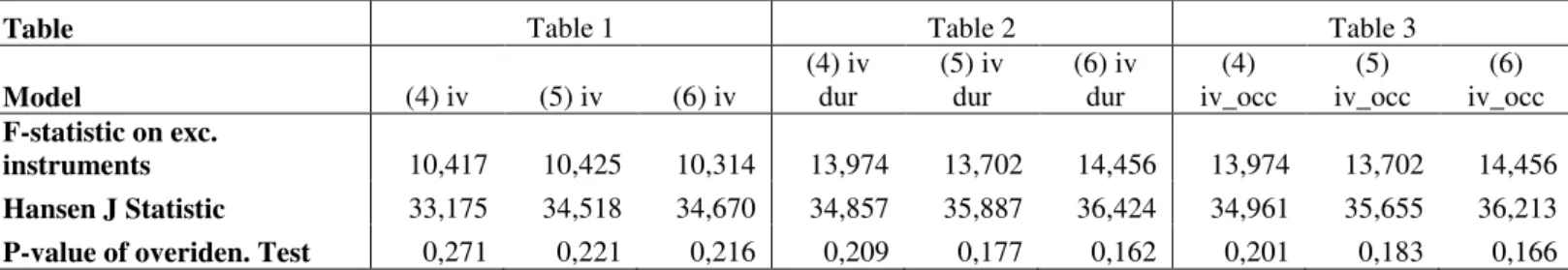
Table 5: Summary of previous tables’ instrument tests (Hansen and K-Paap Test)
Table 6: Test hypothesis θiv ≠ θols.
Table 7: Test hypothesis θheckman≠ θols. Heckman model considers the first step probability of migrating and returning (individuals older than 17 years-old) whose controls are age, age square, education, marital status, number of children and gender. The second step has exactly the same controls as the ols regression
Table 1 Table 2 Table 3
ols (1) vs iv (4) ols (2) vs iv (5) ols (3) vs iv (6) ols (1) vs iv (4) ols (2) vs iv (5) ols (3) vs iv (6) ols (1) vs iv (4) ols (2) vs iv (5) ols (3) vs iv (6) p-value 0,168 0,2372 0,1259 0,7177 0,8912 0,5646 0,5353 0,6538 0,4946
Table 1 Table 2 Table 3
9 Annex 2: Borjas and Bratsberg Model (1996)
The model created by Borjas and Bratsberg explains the relation between unobserved characteristics and decision of migrating and returning. The reasoning behind migrating may be increasing productivity abroad and come back home to get the returns; migrants can decide to stay abroad for ever. Both possibilities have the same goal: Maximize life-cycle earnings.
Individual’s human capital is composed by two parts: one that depends on observed
characteristics (age, schooling, etc) and one depending on unobserved factors such as courage, risk aversion (component v in the models). The return of each factor will change depending on where the individual is (home or abroad).
1) Whome = Ωhome(X) + v
2) Wabroad = Ωabroad(X) + ρv + ε
Where W refers to life-cycle earnings at home or abroad; Ω is a component that comes from observed characteristics, v is a component that comes from unobserved
characteristics and ε and wage’s uncertainty component. The ε only exists in the wage equation while abroad because one assumption of model states that individuals have uncertainty about wages before migrating (period when they decide whether they migrate).
When considering that individuals have productivity gains after a period abroad, the post-migration wage equation would be:
10
Life cycle earnings would be a linear combination between life-cycle earnings abroad and the ones at home plus productivity gains. It would not make sense to work at home before migrating (productivity gain assumption holding).
4) Whome&abroad = ∂ *Wabroad + (1-∂)*(Whome + k), where Whome&abroad is life-cycle
earnings in a combination between home and abroad; ∂ is the fraction of
working life abroad and k is the productivity gain abroad.
The authors also consider that there is a fixed cost of Migration (M) and Returning (R). A risk-neutral individual migrates when:
i) Expected(Wabroad) – M > Whome
ii) Expected(Whome&abroad) – M – R > Whome And he/she return home if:
iii) Conditions i) and ii) hold
iv) Whome – R > Wabroad; meaning that expectations according to earning abroad were not correct
v) Expected(Whome&abroad) – R >Waboard; Productivity gains at home make return optimal.
With the previous model the authors are able to sort individuals by unobserved characteristics:
Stay in the origin country:
(1-ρ)v ≤ (Ωhome(X) - Ωabroad(X) + k) + (𝑴 + 𝑹 − 𝒌)/𝛛
Migrating:
11
Returning to the origin country:
(Ωhome(X) - Ωabroad(X) + k) + (𝑴 + 𝑹 − 𝒌)/𝛛 < (1-ρ)v ≤
≤ (Ωhome(X) - Ωabroad(X) + k) - 𝑹
𝟏−𝛛− 𝜺
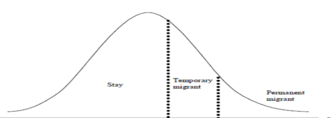
While considering no uncertainty on wages abroad (ε = 0), unobserved characteristics determines who migrate. With unobserved characteristics are better paid abroad (ρ higher than 1), migrants will be individuals highly skilled in terms of unobserved characteristics and return migrants have incentives to migrate only temporary. So return migrants will be between migrants and non-migrants in terms of ability (ρ).
Figure 1: Ability’s distribution and decision to migrate, from Lacuesta (2006)
The opposite conclusion will be taken if unobserved characteristics are better paid at home, the permanent migrants would be the individual with lower ability (v).
12 E(v|nonmig)</>E(v|retmig) </>E(v|nonretmig)
Positive selection in unobserved characteristics is reflexed by migrants having more ability than non-migrants.
Negative selection happens in opposite cases: return migrants have lower ability than non-migrants.
When the authors introduce the uncertainty component, the decision of migrating does not change but the period of migration may change. Some migrants may realize that migration is not as optimal as they though and they may decide to stay shorter periods. Return migrants continue to be in the middle of migrants and non-migrants in terms of unobserved characteristics.
14
Annex 3: Full Survey, English Version
Subject Recruitment and Corresponding Participation Consent
Good Morning/Good Afternoon.
I am part of a team conducting a study about the opinion of the population of CV on the quality of the public services in the last 20 years and the characteristics of the population concerning migration.
Approximately 1000 interviews will be conducted. You have been selected randomly and will only provide your name only if that is your wish (your name is not important for the study).
This study may be a valuable instrument for the improvement of the public services in CV.
Each interview has the approximate duration of 30 minutes.
This questionnaire is to be used in a research/scientific study. The initiative and conduction of this project is the sole responsibility of the University of Oxford, United Kingdom. This institution is totally independent of the institutions of CV, including its government.
The Ministry of Education of Cape Verde is informed of the conduction of this study. The Statistics Office of Cape Verde is informed and has agreed on the realization of this study.
Total anonymity is guaranteed upon request.
Any contact for pertinent answers about the research and research subjects’ rights should be directed to:
Dr. Pedro Vicente (research team leader) Email: [email protected] Tel. +44-1865-281446
Center for the Study of African Economies Department of Economics
University of Oxford
Manor Road Building, Oxford OX1 3UQ United Kingdom
Participation in this study is voluntary. Refusal to participate will involve no consequence to the subjects of this study. The subject may discontinue participation at any time without penalty or loss of benefits to which he or she is otherwise entitled.
15
QUESTIONNAIRE
Instructions:
The questions of the questionnaire are mainly related with past impressions. We are going to ask you a memory effort. For us to be able to help you, we are going to ask some general questions regarding your past. With that information, we will be able to guide you in the questions regarding your opinions about the public services in the last 20 years.
(TO BE COMPLETED BY THE INTERVIEWER)
#: __________________
INTERVIEWER: __________________
DAY: __________________
STARTING TIME: __________________
PLACE: __________________
ABILITY TO ANSWER THE QUESTIONNAIRE
Instructions: Firstly we are going to ask you a set of questions aimed at assessing if you are in position to help us.
1. This year are you 30 years or older? (AGE30)
Yes 1 No 0
IN CASE OF DOUBT ASK:
Were you born on the independence of CV in 1975?
Were you born on April 25th 1974 (Portuguese Revolution)? 2. Personal History
BEGIN BY ASKING:
Have you been a resident of CV in the last 20 years?
1985-1988 «end of single party»
2.1.1. Were you a resident of CV? (DPRES1)
Yes 1 No 0
IF NOT
2.1.2. Were your direct (Parents, Husband/Wife, Children) relatives resident in CV? (IPRES1)
Yes 1 No 0
1991-1997 «beginning of democracy»
2.2.1. Were you a resident of CV? (DPRES2)
Yes 1 No 0
IF NOT
2.2.2. Were your direct (Parents, Husband/Wife, Children) relatives resident in CV? (IPRES3)
Yes 1 No 0
2000-today «last 5 years»
2.3.1. Were you a resident of CV? (DPRES3)
Yes 1 No 0
IF NOT
2.3.2. Were your direct (Parents, Husband/Wife, Children) relatives resident in CV? (IPRES3)
Yes 1 No 0
THE INTERVIEW CONTINUES ONLY IF THE SUBJECT IS MORE THAN 30 YEARS OF AGE AND ANSWERS YES TO AT LEAST ONE QUESTION IN EACH TIME PERIOD.
16 RELAXING QUESTIONS
Instructions: You are in position to help us! Before asking some questions about your past, we would like to ask you general questions on your current general opinion about several public services.
1. How do you rate the general quality of the following public services?
---BAD--- ---GOOD---
Extremely Very Slightly Neither good Slightly Very Extremely NA
bad nor bad good
1.1. Health (HEA)
1 2 3 4 5 6 7 -1
1.2. Education (EDUC)
1 2 3 4 5 6 7 -1
1.3. Courts (TRIB)
1 2 3 4 5 6 7 -1
1.4. Police (POLI)
1 2 3 4 5 6 7 -1
1.5. Licensing Services (BURO)
1 2 3 4 5 6 7 -1
1.6. Fight Against Poverty Programs (POV)
1 2 3 4 5 6 7 -1
1.7. Customs (CUST)
1 2 3 4 5 6 7 -1
1.8. Migration Services/Passport Emission (PASS)
1 2 3 4 5 6 7 -1
1.9. Water and Electricity Company Electra (WAT)
1 2 3 4 5 6 7 -1
1.10. Post Office (POST)
1 2 3 4 5 6 7 -1
1.11. Telecommunication Services CV Telecom (PHO)
1 2 3 4 5 6 7 -1
2. "Good times were those when you were young". (OPTIM1)
---DISAGREE--- ---AGREE---
Disagree Neither agree Agree
Totally Strongly Slightly nor disagree Slightly Strongly Totally NA
7 6 5 4 3 2 1 -1
3. "The future of CV will be better than the present." (OPTIM2)
---DISAGREE--- ---AGREE---
Disagree Neither agree Agree
Totally Strongly Slightly nor disagree Slightly Strongly Totally NA
1 2 3 4 5 6 7 -1
BASIC DEMOGRAPHY
Instructions: We are then going to ask you several questions regarding you and your past.
1. How many children have you had until today (including those who died after being born alive)? (CHILDN)
NA -1
2. What are the ages of your children this year? (Begin with the oldest; if any already dead, tell us age in the year of death and year of death)
FILL YOB WITHOUT ASKING (CHILDA)
3. Went to primary school 1-4? 4. Went to secondary school 5+?
IF YES AND 5 OR LESS CHILDREN, FILL WITHOUT ASKING:
(CHILDSC) (CHILDSE)
YOB+6: YOB+10: YOB+18: