Coupling of the FLake model to the Surfex externalized surface model
14
0
0
Texto
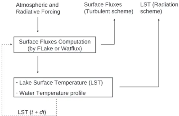
(2) 232. Salgado & Le Moigne • Boreal Env. Res. Vol. 15. Portugal, where the Alqueva dam was built. The impact of this human activity on local climate has been recognized for some time (e.g. Anthes 1984, ICOLD 1994) and there is a possibility that feedbacks between the mesoscale circulations forced by the modified surface and the surface fluxes of latent and sensible heat, can lead to changes in the surface water budget, cloud cover or even in convective precipitation. Anyway, an improved representation of the lake physical processes is needed in order to improve our understanding of the water balance in the Mediterranean climate. The current generation of mesoscale and weather forecast models doesn’t include an explicit representation of the evolution of lake temperature, which is most of the time maintained constant over the integration period. An accurate prescription of lake surface temperatures becomes more important as the horizontal resolution of the weather forecast models increases. Surface modelling in numerical weather prediction has always held an important place in the activities of the Centre National de Recherches Météorologiques (CNRM hereafter). In the late 1980s, ISBA (Interaction between Soil Biosphere and Atmosphere) — a soil–vegetation–atmosphere transfer scheme — has been developed (Noilhan and Planton 1989). Its aim is to better simulate the exchanges of energy and water between the land surface and the atmosphere just above. More recently, modelling of urban areas has began to be of great interest in the research community and CNRM. In 2000, TEB (Town Energy Balance) model, specially designed to represent the exchanges between a town and the atmosphere at the mesoscale, has enabled advanced studies in this direction (Masson 2000). As far as modelling of water surfaces is concerned, schemes of different complexities are available. For example, a one-dimensional ocean mixing layer model (Lebeaupin 2006) aims to improve the simulation of the sea-surface temperature (SST hereafter) and the induced fluxes. The FLake model (Mironov 2008) has shown its ability to model the evolution of lake surface temperature with the accuracy and the efficiency required in numerical weather forecast.. The improvement of water surface temperature increases the accuracy of the heat and mass fluxes computation at the water–atmosphere interface. A special effort has been made this last years at CNRM to externalize the surface scheme from the original embedded surface–atmosphere system. The main idea was to gather all the developments and improvements made in surface schemes in order to make them available for as many people as possible. Not only have physical parameterizations been externalized, but also the preparation of specific surface parameters needed by the physical schemes and the initialization of all state variables of the different models. The result of the externalization has led to the Surfex system which contains several independent models like ISBA, TEB and the one-dimensional ocean mixed layer model above mentioned. This paper shows how FLake model has been implemented into Surfex system and describes its evaluation on the Alqueva lake datasets.. Model description Surfex In Surfex, the exchanges between the surface and the atmosphere are realized by mean of a standardized interface (Polcher 1998, Best et al. 2004) that proposes a generalized two-way coupling between the atmosphere and the surface. During a model time step, each surface gridbox receives the upper air temperature, specific humidity, horizontal wind components, pressure, total precipitation, long-wave radiation, shortwave direct and diffuse radiations and possibly concentrations of chemical species and dust. In return, Surfex computes averaged fluxes for momentum, sensible and latent heat and possibly chemical species and dust fluxes and then sends these quantities back to the atmosphere with the addition of a radiative surface temperature, surface direct and diffuse albedo and also surface emissivity. All this information is then used as lower boundary conditions for the atmospheric radiation and turbulent schemes (Fig. 1). One of the idea of Surfex is to split each model gridbox into fractions of sea, lake, urban and natural.
(3) Boreal Env. Res. Vol. 15 • Coupling FLake to Surfex. Fig. 1. Exchange between an atmospheric model sending meteorological and radiative fields to the surface and Surfex composed of a set of physical models that compute tiled variables Фn, Фl, Фt and Фs covering respectively fractions fn, fl, ft and fs of a unitary grid box and an interface where the averaged variables Ф are sent back to the atmosphere.. areas. The coverage of each of these surfaces is known through the global ECOCLIMAP database (Masson et al. 2003), which combines land cover maps and satellite information. Each surface type is simulated with a specific surface model (ISBA for natural areas, TEB for urban areas, FLake or Watflx for lakes and Watflx for seas) and the total flux of the grid box results from the addition of the individual fluxes weighted by their respective fraction. The ISBA scheme has been designed to be simple and efficient in order to be used in many operational atmospheric models. The ISBA scheme computes the exchanges of energy and water between the continuum soil–vegetation– snow and the atmosphere above. In its initial version, the evapotranspiration of the vegetation is controlled by a resistance like proposed by Jarvis (1976). A more recent version of the model named ISBA-A-gs (Calvet 1998) accounts for a simplified photosynthesis model where the evaporation is controlled by the aperture of the stomata, the component of the leaves that regulates the balance between the transpiration and the assimilation of CO2. Nowadays, the ISBA. Φn. fn. 233. Φ = fnΦn + flΦl + ftΦt + fsΦs Φl. Φt. Φs. fl. ft. fs. land surface scheme is used in the French operational and research forecast models. The TEB model is based on the canyon concept (Oke 1987), where a town is represented with a roof, a road and two facing walls with characteristics playing a key role in the town energy budget. More especially, the ability of the canyon to trap a fraction of the incoming solar and infrared radiation is taken into account in the model. The representation of water surfaces has also been improved. Indeed, up to now, the exchanges of energy between water surfaces and the atmosphere were treated in a very simple way, while now physically based model have been introduced to build a more complex but accurate surface model, available for all atmospheric models. There are two possibilities to compute fluxes over marine surfaces. The simplest one consists in using Charnock’s approach to compute the roughness length and fluxes with a constant water surface temperature during the simulation period. Secondly, a one-dimensional ocean mixing layer model has been introduced in order to simulate more accurately the time.
(4) 234. Salgado & Le Moigne • Boreal Env. Res. Vol. 15. evolution of the sea surface temperature and the fluxes at the sea–air interface. This model based on Gaspar (1990), helps, especially at the mesoscale, to represent diurnal cycle of SST (Lebeaupin 2006). A better restitution of lake surface temperature and consequently of the associated surface fluxes is also the main improvements expected by the use of the FLake model.. defined by its integral between ζ = 0 and ζ = 1, which is the shape factor CT. So, the water temperature profile assumed by FLake is completely described by four variables: TS, TBOT, h and CT and one fixed parameter: D. The set of FLake variables includes also the mean temperature of the water column TMEAN, but there are only four independent water variables, and therefore four prognostic equations. Two of them are the energy balance equations for the mixing layer and for the total water column. To represent how the short-wave radiative heat flux penetrates into water, FLake uses the commonly used exponential approximation of the decay law. Several spectral bands characterized by different extinction coefficients depending on water turbidity may be considered. The evolution of h is computed using a sophisticated formulation, that treats both convective and stable regimes and accounts for the vertical distribution of the radiation heating. In the first case, the evolution of the depth h of the convective mixed layer is computed by an entrainment equation. Under stable and neutral stratification, the wind-mixed layer depth h is computed by a relaxation-type equation. The shape factor, CT varies between a minimum value, CTmin = 0.5, corresponding to a mixed layer stationary state or retreat, and the maximum value CTmax = 0.8, the maximum curvature in the mixed layer deepening process. CTmin = 0.5 is consistent with a linear temperature profile that is assumed to occur for shallow lakes under the ice cover when the bottom temperature is less than the temperature of maximum density (Tr = 4 °C; Mironov 2008), in this case, the heat flux at the bottom is from the sediments to the lake water. The value CTmax = 0.8 is greater than the originally proposed one, to accommodate recent observational results, particularly those shown in Kirillin (2001). The evolution of CT is computed using a relaxation type rate equation with a relaxation time which is proportional to the square of the thermocline thickness (D – h)2. FLake includes also an optional module that simulates the evolution of the vertical temperature structure of the thermally active layer of bottom sediments and its interaction with the water column. The thermal vertical structure in this layer is described using the same concept of. FLake The model is intended for use as a lake parameterization scheme in numerical weather prediction, climate modelling, and other numerical prediction systems for environmental applications. FLake can also be used as a stand-alone lake model, as a physical module in models of aquatic ecosystems, and as an educational tool. The lake model TeMix proposed by Mironov et al. (1991) was taken as a starting point for the development of FLake, which is a lake bulk model, fully documented in Mironov (2008). It is based on a two-layer parametric representation of the evolving temperature profile and on the integral budgets of heat and kinetic energy for the two layers. The structure of the stratified layer between the upper mixed layer and the basin bottom, the lake thermocline, is described using the concept of self-similarity of the temperature-depth curve. This concept, based on empirical evidence with some theoretical support, assumes that the dimensionless temperature profile follows an assumed shape function of dimensionless depth: (1) where TS is the mixed-layer surface temperature, TBOT the temperature at the lake bottom, h the thickness of the mixed-layer and D the total lake depth. D – h is the thermocline depth. Several polynomial approximations for ФT may be found in the literature (see Mironov 2008) and some authors (e.g. Mälkki and Tamsalu 1985) noticed that the shape function is different when the depth of the mixed layer increases than when it decreases. In FLake, a 4th order polynomial is assumed for ФT and its shape is completely.
(5) Boreal Env. Res. Vol. 15 • Coupling FLake to Surfex. 235. self-similarity. On top, FLake contains a snowice module which is not used in the present study. Implementation The FLake model has been implemented into Surfex. The models are coupled explicitly through an interface that calls the FLake routines inside a do loop over the horizontal grid points where lakes are present. During a time step (Fig. 2), the surface fluxes of momentum and of sensible and latent heat are computed before FLake variables, particularly the lake surface temperature (LST hereafter). These fluxes may be computed using the routines provided by FLake (SfcFlx routines described in Mironov 1991) or by the Watflux scheme used usually in Surfex. Then FLake computes the new LST, which will be used at the next model time step t + dt and also as boundary condition for the atmospheric radiation scheme. The use of FLake inside Surfex requires additional spatialized parameters. Firstly, the fraction of each grid box covered by lakes has to be known. In Surfex, the lake fractions are mapped, by default, by means of the ECOCLIMAP database (nominal resolution of 1 km). Secondly, using FLake requires the initialization of variables that evolve in time as well as constant parameters (see Table 1), for all grid boxes which contain a non zero lake fraction. For numerical studies, when these values are known over the area of interest or even partially unknown over some regions of the domain, default values are applied. For that reason, the development of a global lake database would be of high interest, especially to give information on the average depth and the extinction coefficient of solar radiation, the two main parameters to which the model is sensitive. Whenever this information is not available, a lake depth of 20 m and an extinction coefficient of 3 m–1 are provided as default values to the Surfex_FLake. LST (t + dt). Fig. 2. Schematic diagram showing the coupling between the atmosphere and the Surfex_FLake system.. model. Albedo and emissivity default values are taken from the Watflux Surfex scheme. Surfex lake temperature TS may be initialized from climatology, large scale analysis or forecast. In the last case, as the French large-scale model does not contain actually lake information, TS is approximated by the deep temperature of the nearest land point. When TS is greater than the temperature of maximum density Tr = 4 °C, the default initial thermal profile is assumed to be not stratified and TBOT = TS, which is not convenient for short period simulations, specially in Summer. When TS is lower than Tr, the initial bottom temperature is set to TBOT = Tr and the default profile is assumed to be characterized by CT = 0.5. By default, the mixed layer depth is initialized to h = 3 m. The mean water temperature TMEAN is computed from TS, TBOT, h and CT. Finally, when the sediment module is activated, the depth of the thermally active sediments layer is fixed by default to 50 cm. Note that the default values are arbitrary, and for simulations where the lake effects are expected to be important, more realistic initial values and parameters need to be given in order to have a better representation of air–lake interactions. In this paper, the coupled model will be called Surfex_FLake. The first techni-. Table 1. Most important FLake parameters and default values used in the Surfex implementation. Parameter Lake depth, D Extinction coefficient Default values. 20 m. 3 m–1. Fetch Sediments depth Albedo Emissivity 1000 m. 1 m. 0.135. 0.98.
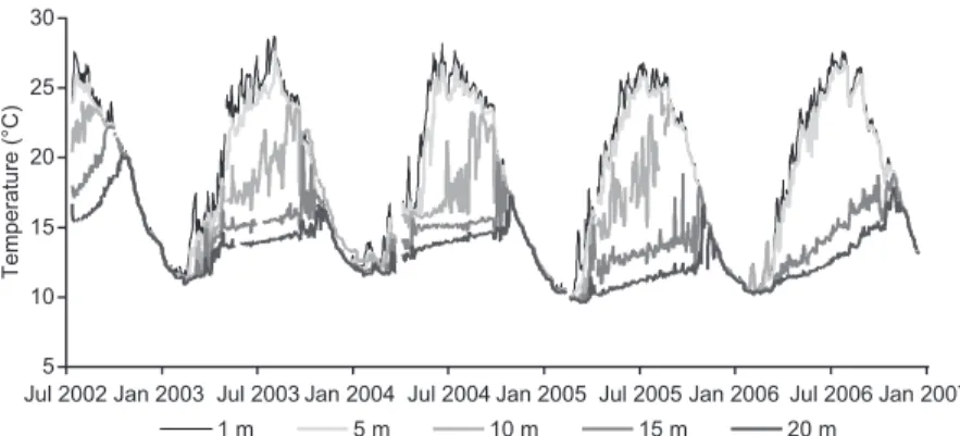
(6) Salgado & Le Moigne • Boreal Env. Res. Vol. 15. 236. Fig. 3. Location of the Alqueva reservoir. The orography of the zoomed region is represented with contour intervals of 100 m. The localization of the experimental station is indicated by the star.. cal validation was to verify that the results of Surfex_FLake on a point completely covered by water were identical to those produced by FLake alone. The results showed that Surfex_ FLake and FLake alone integrations gave the same results, with only small differences due to numerical approximations (not shown).. Data collection Site description The Alqueva reservoir when completely filled covers an area of about 250 km2 (Fig. 3) and its volume is about 4 250 106 m3, which leads to an average depth of 16.5 m. In this reservoir, the Portuguese Water Insti-. tute (INAG, the Portuguese water authority) installed in July 2002 two meteorological and hydrological stations on floating platforms, as part of a monitoring network of the reservoirs in southern Portugal. Data from the station named Alqueva station, located at 38.22°N, 7.46°W (Fig. 3), are used in this work. The meteorological station, mounted over the floating platform, includes measurements of air temperature, air moisture, wind speed and direction, downward solar radiation, pressure and precipitation. All variables are measured in 10-s intervals and afterwards averaged to 15-min values, except for precipitation which is accumulated during the period. In addition, water temperature was continuously measured at five different levels (1, 5, 10, 15 and 20 m). The station included also measurements of water quality parameters, not used in the present study. The data from the weather station was used to force long off-line FLake runs, while the water temperature data was used to validate those runs (see below). The thermal regime of the lake is characterized by the existence of a stratified period which starts usually in the beginning of March and ends in November (Fig. 4). In winter, the water thermal profile is not stratified and the temperature decreases, reaching minimum values of 10 to 11 °C. In summer, close to the surface, temperature regularly exceeds 27 °C. The instantaneous water temperature near the surface can even exceed 30 °C in the afternoon. During the period of greatest stratification, the difference between temperatures at the depths of 1 meter and 20 meters reaches typically 15 °C.. Temperature (°C). 30 25 20 15 10 5 Jul 2002 Jan 2003 Jul 2003 Jan 2004 Jul 2004 Jan 2005 Jul 2005 Jan 2006 Jul 2006 Jan 2007 1m. 5m. 10 m. 15 m. 20 m. Fig. 4. Evolution of daily mean water temperatures observed at 1-m, 5-m, 10-m, 15-m and 20-m depths in the Alqueva reservoir..
(7) Boreal Env. Res. Vol. 15 • Coupling FLake to Surfex. Intensive field campaign As mentioned above, the Alqueva station doesn’t include measurements of near surface fluxes, which are important for validation of the lake models from the point of view of atmospheric modelling. To address the lack of flux data, we set up an intensive field-observation campaign supported by the Universities of Lisbon and Évora, the INAG and the EDIA (the public company responsible for the management of the Alqueva reservoir). The field experiment was performed between 10 July and 5 September 2007. Eddy-correlation (EC hereafter) measurements were carried out from the above-mentioned instrumented floating platform. Variables measured were u, v and w components of wind speed, the acoustic temperature (computed from the measured sound speed) and the absolute humidity. The fast-response instrumentation consisted of an ultrasonic anemometer (Metek, model USA-1) and an open path krypton hygrometer (Campbell Scientific, model KH20). Measurements were made at a frequency of 20 Hz and the covariances were computed for every 15-min period. The fast-response instruments were mounted on a boom, 5 m from the station mast, at a height of 2 m above the water surface. The horizontal distance between the hygrometer and the vertical sonic path was 10 cm, the value recommended by Campbell (1985) to avoid the need for any adjustment for sensor separation. The raw data were acquired and archived on a laptop computer. Attendance at the eddy correlation system was mainly required to check the quality of the data and to clean the hygrometer sensor. Post-processing of the eddy-covariance data included rotation of coordinates of the wind component data to set the ensemble averages of w to zero. In order to minimize the errors associated with low frequency trends, all signals were linearly de-trended in each 15-min segment. Unrealistic humidity values, frequently caused by the existence of water drops covering the optical window of the hygrometer, were rejected. In addition, in order to have all terms of the energy balance equation, radiation measurements were taken from another mast on a. 237. floating platform. For short wave measurements we used one dual pyranometer (Phillip Schenk, model 8104). The total, descendent and ascendant radiative fluxes were measured with one pyrradiometer (Phillip Schenk, model 8111). Long wave flux is obtained by difference between total and short wave radiative fluxes. Radiative variables were measured in 10-s intervals and afterwards averaged to 15-min values, which were then stored on a data logger (CR10X, Campbell Scientific Inc.). Excluding erroneous moisture data records, and after the quality control process, we collected a total of 18 and 53 days with complete data series of latent and sensible heat fluxes, respectively. With respect to screen level meteorological variables and to short and long wave radiation fluxes, the data series did not contain evident measurement errors and all the 56 days of the campaign could be used. During the intensive field campaign, water temperature at depths 1 m, 15 m and 20 m were logged every 30 minutes. In addition, water temperature near the bottom reservoir were available at the same time frequency.. Long runs and model adjustments In the first step, the FLake model was tested over the years 2002 to 2006 in an off-line mode, forced by time series of the hourly averaged variables — pressure, air moisture and temperature, wind speed and solar global radiation — collected at the Alqueva station. As not measured at the station, the long wave radiation, also needed as input of the model, was extracted from the ECMWF analysis. As the model required complete time series, missing data were replaced by values obtained by linear interpolation, when the gap was smaller than three hours or, if it was greater, data recorded at neighbouring stations were used, after corrections based on linear regression between the stations. The first tests showed a strange behaviour in the evolution of simulated thermal profile, starting at the beginning of the warming period (Fig. 5). Unlike expected evolution, the simulated water deep temperature decreases in spring, reaching the temperature of maximum density. It.
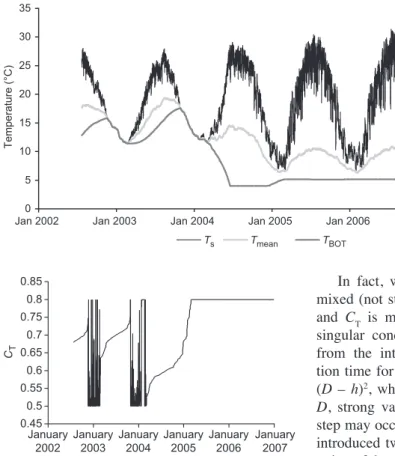
(8) Salgado & Le Moigne • Boreal Env. Res. Vol. 15. 238 35. Temperature (°C). 30 25 20 15 10 5 0 Jan 2002. Jan 2003. Jan 2004 Ts. Jan 2005 Tmean. 0.85 0.8 0.75 CT. 0.7 0.65 0.6 0.55 0.5 0.45 January January January January January January 2002 2003 2004 2005 2006 2007. Fig. 6. FLake model offline results for daily mean shape factor CT.. was found that the year when this effect appears, depends on the choice of parameters. We found that this type of behaviour is linked to the fact that sometimes, when the temperature of the surface begins to increase and the profile of water is beginning to stratify, the shape factor “jumped” to a very low value, close to its lower limit of 0.5. With this value and the associated profile, an increase of the surface water temperature and of the mean water temperature may lead to a decrease of the bottom water temperature. As the evolution of CT is slow (Fig. 6), during the heating period, the deep temperature decreases to a value close to the value of maximum density (Fig. 5). Later, in the cooling period, as the value of the simulated TBOT is very low, the mixing layer does not reach the bottom. So the thermal stratification is maintained throughout the year and the deep temperature does not increase. The model thus tends to create a perpetual stratification which departs from reality.. Jan 2006 TBOT. Jan 2007. Fig. 5. FLake model offline results for daily mean surface temperature TS, mean temperature TMEAN and bottom temperature TBOT.. In fact, when the lake water is completely mixed (not stratified), TS = TBOT = TMEAN, h = D and CT is meaningless. Numerically, near this singular condition, CT may assume any value from the interval 0.5–0.8 and, as the relaxation time for the CT evolution is proportional to (D – h)2, which tends to zero, when h tends to D, strong variations of CT in one model timestep may occur. To overcome this behaviour, we introduced two small changes in the implementation of the model: first, we fixed the value CT at 0.65 in warm, non-stratified conditions, instead of the original value of 0.5, which is appropriate to describe thermal profiles of frozen lakes; secondly, we constrained ΔCT (the variation of CT) to a maximum value |ΔCTmax| = CM ¥ Δt, where Δt is the model time step, and CM is a constant tentatively estimated to be 0.01 h–1. When the temperature profile is not stratified at all and the temperature is above the temperature of maximum density, changing the value of CT to 0.65 makes the model simulate a more realistic profile at the beginning of the stratification period. The constraint imposed on the rate of change of CT prevents sudden jumps in the vicinity of the numerically singular point when the stratification starts and (D – h) is close to zero. It has no effect on stratified profiles. The impact of these two small changes lead to a slight increase of the shape factor during the heating period, starting from 0.65 and reaching values close to 0.8 (its highest limit) at the end of summer. In connection with the shape factor trend, the thermal gradient is very high just below the mixing layer during the stratified.
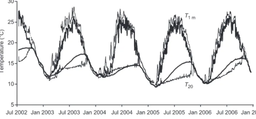
(9) Boreal Env. Res. Vol. 15 • Coupling FLake to Surfex. 239. 30 T1 m. Temperature (°C). 25. Fig. 7. Observed and simulated daily mean water temperatures at 1-m and 20-m depths in the Alqueva reservoir.. 20 15 10. T20. 5 Jul 2002 Jan 2003 Jul 2003 Jan 2004 Jul 2004 Jan 2005 Jul 2005 Jan 2006 Jul 2006 Jan 2007. period and the simulated bottom water temperature evolves smoothly, remaining almost constant in spring and increasing slightly in summer and early autumn. In autumn, normally in November, the lake stratification disappears and the lake temperature decreases as a block during the cooling period. Thus, with these minor changes, the model describes realistically the temporal evolution of lake temperature at various depths (Fig. 7).. Tuning of FLake parameters The FLake model contains free parameters (Table 1) with a range of plausible values. After some sensitivity tests, we found, in accordance with Kourzeneva (2005), that, among the various parameters, the model is more sensitive to the lake depth and, to a lesser extent, to the extinction coefficient of the light. The water optical properties were not measured and the model depth in our case is difficult to estimate because of the topographical characteristics of the lake. In this study, it is seen as an effective or spatially-averaged parameter and not a local one. In order to find a set of optimal values for the model parameters, the model was calibrated. For long periods of simulation, the calibration of lake depth and extinction coefficient consisted in minimizing the root mean square error of daily average water temperature observed and simulated at different depths. In this case, the water temperature profile was initialized by observations. However, the influence of the lake initial state vanishes rapidly enough in time and doesn’t require a very strong accuracy. On the. Surfex_FLake. Obs.. other hand, for short range simulations, not only lake depth or extinction coefficient of light were calibrated but also the initial water temperature profile (including mixing depth and shape factor) by taking into account also the hourly average of sensible and latent heat fluxes. As in atmospheric modelling, the crucial point is to correctly compute the surface fluxes, in the statistical analysis we gave more weight to the accuracy in the first water temperature level and, for the shorter intensive observation period, the weight of sensible heat flux was predominant. The statistical analysis is based on the classical computation of mean error (bias), root mean square error (RMSE) and correlation coefficient (R) which involves observations (Y ) and simulations (X ): (2) (3) (4) where (X, σX) and (Y, σY) are respectively the mean and standard deviation of the simulated and observed values.. Results The Surfex_FLake system in the off-line mode was used for the simulations, considering only one grid point, totally covered by water. As mentioned above, after the changes in the shape factor computation, the long-term evolu-.
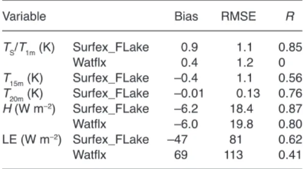
(10) 240. Salgado & Le Moigne • Boreal Env. Res. Vol. 15. tion of the reservoir water thermal profile is well simulated by the FLake model in the five-years integration experiment. The results (Fig. 7) correspond to a tuned simulation with a total depth of 30 meters and an extinction coefficient of 4 m–1. For clarity, we present only the comparison of temperatures observed and simulated at the first and at the last observational levels. The comparison indicates that the model is capable of simulating the annual pattern of the thermal profile, correctly capturing the transition between the stratified and the well mixed periods. The temperature of the lake in winter (no stratified periods) is particularly well simulated. On the other hand, the pattern of the evolution of deep temperature (20 m) during the summer is not well simulated. Even if the annual minimum and maximum temperatures are correctly captured, at this depth, the model temperatures increase earlier than the observed ones. Note that FLake uses an effective depth and attempts to represent a horizontally average profile, while the observations are local and, in this case, were taken in a place where the lake has a depth of about 60 m. It is not expected that a one-dimensional assumed shape model like FLake can provide detailed water thermal profiles in man-made reservoirs, characterized by high slopes at the bottom. However, this is not a problem for mesoscale weather forecast models, which aim to improve the representation of the surface temperature. The quality of the simulation is quantified by the statistics (Table 2) computed for all observation levels. The high correlations, and small RMSE, also confirm the ability of the model to represent the thermal evolution of the reservoir. However, the near surface simulated temperatures have a negative bias of more than 1 °C.. In the short simulation period (56 days; 10 July to 5 September 2007), the atmospheric forcing, including the downward long-wave radiation flux at the surface, was taken from the field campaign data. After tuning, the following parameters were used: lake depth = 40 m; Extinction coefficient = 3.5 m–1. Using the same formulation for surface fluxes (Surfex one), we carried out two Surfex off-line simulations, one with a constant surface temperature (named Watflx) and the other one (Surfex_FLake) with surface temperature evolving in time. Both Watflx and Surfex_FLake experiments were driven by the same atmospheric forcing and were identically initialized. The initial conditions, constructed from the water measurements at the Alqueva station, were: TS = 298.8 K, TBOT = 285.4 K, CT = 0.77, h = 3.3 m. Since surface temperature does not evolve during the Watflx run, it equals its initial value of 298.8 K. The correlations between simulated and observed temperatures are greater than 0.75 except for the T15m (Table 3). On average, the simulated mixed layer is 0.9 °C warmer than the observed one (Table 3 and Fig. 8) and the daily thermal amplitude is a little higher (on average 1.4 °C versus 1.0 °C). The signal of the surface temperature bias is the opposite to that found in the five-year simulation (Table 2), due to the use of two different heat-flux schemes. Indeed, the surface fluxes computation in the five-year experiment is the FLake’s one (Mironov 1991) and differs from the Surfex original formulation. The comparison between the two formulations will not be addressed in this paper. Note that for. Table 2. Summary of statistics for daily mean water temperatures at different depths simulated by FLake (2002–2006). Depth (m) 01 05 10 15 20. Bias (K) RMSE (K) –1.28 –1.61 –1.24 0.08 0.62. 1.73 2.18 2.05 1.23 1.40. R 0.98 0.98 0.91 0.88 0.84. Table 3. Summary of statistics for hourly mean water temperatures and surface heat fluxes simulated by Surfex_FLake for the period 10 July–5 September 2007. Variable TS/T1m (K) Surfex_FLake. Watflx T15m (K) Surfex_FLake T20m (K) Surfex_FLake H (W m–2) Surfex_FLake. Watflx LE (W m–2) Surfex_FLake. Watflx. Bias RMSE 0.9 0.4 –0.4 –0.01 –6.2 –6.0 –47 69. 1.1 1.2 1.1 0.13 18.4 19.8 81 113. R 0.85 0 0.56 0.76 0.87 0.80 0.62 0.41.
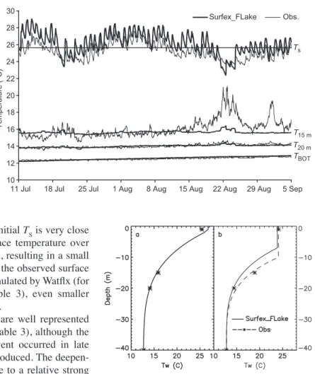
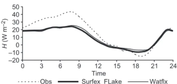
(11) Boreal Env. Res. Vol. 15 • Coupling FLake to Surfex. 241. 30. Surfex_FLake. 28 26. Obs.. Ts. Temperature (°C). 24. Fig. 8. Hourly water temperatures observed and simulated by Surfex_ FLake at 1-m, 15-m, 20-m depths, and at the bottom in the Alqueva reservoir.. 22 20 18 16. T15 m. T20 m TBOT. 14 12 10 11 Jul. 18 Jul. 25 Jul. the period considered, the initial TS is very close to the mean observed surface temperature over the entire simulation period, resulting in a small bias between time series of the observed surface temperature and the one simulated by Watflx (for which TS is constant) (Table 3), even smaller than the Surfex_FLake bias. The deep temperatures are well represented by the model (Fig. 8 and Table 3), although the mixing layer deepening event occurred in late August is not correctly reproduced. The deepening of the mixing layer, due to a relative strong wind episode, also appears in the simulation results, where h increases from 2 m at 13:00 on 18 August to the maximum value of 8.7 m at 13:00 on 22 August (Fig. 9), but not sufficiently to reproduce the observed increase in water temperature at 15-m depth. Unfortunately, the lack of temperature measurements at 5 m and 10 m prevents us from giving a fine diagnostic of the mixing layer deepening. But the deep-temperature increase could be correctly simulated by the model with a mixed layer thickness of about 10.5 m (Fig. 9): a relatively small error in the calculation of h due probably to two-dimensional effects not represented by the model, leads to a relatively large error in the temperature at this depth. To facilitate the analysis of the latent and sensible heat fluxes, we calculated the mean daily cycles produced by the model, corresponding to the days where observational data are available (Fig. 10). The model captures the pattern of daily evolution of the surface sensible. 1 Aug. 8 Aug. 15 Aug. 22 Aug. 29 Aug. 5 Sep. Fig. 9. Water temperature profiles simulated by Surfex_ FLake and observed at 13:00 UT as a function of depth on (a) 18 August 2007 and (b) 22 August 2007. The dashed line in b represents the FLake profile adjusted to the measured values (h = 10.5 m, CT = 0.8).. heat flux, showing that it is positive during the night and morning, with a maximum at 09:00 UT, and negative in the afternoon. The results are very close to the observations during the afternoon and early evening, but not during the morning when the model values are lower. In the simulations, the low values of sensible heat flux during the night and early morning are a consequence of low values of the roughness length (order of 10–5 m), calculated by the Charnock relation in weak wind conditions. These results confirm the need to improve the calculation of heat fluxes over water surfaces in Surfex, in connection with the recent improvements made in the fluxes calculation over the ocean (Lebeaupin.
(12) Salgado & Le Moigne • Boreal Env. Res. Vol. 15. 242. LE (W m–2). 300 250 200 150 100 50 0. H (W m–2). 50 40 30 20 10 0 –10 –20. 0. 3 Obs. 6. 9. 12 15 Time Surfex_FLake. 18. 21. 24. Watflx. Fig. 10. Mean daily cycles of observed and modelled (FLake and Watflx) sensible heat fluxes.. 2007). This results in an average underestimate of the sensible heat flux of 6.2 W m–2 (Table 3), corresponding to a daily average decrease of about 40%. The comparison with the simulation without the lake model does not show a significant difference, although there is a small improvement in the RMSE and in the correlation parameter. Note that, in this case the surface temperature imposed on the Watflx is very close to the mean surface temperature observed during the integration period. Concerning the surface latent heat flux, we found that the model simulates lower values than those observed with the EC system (Table 3), although the pattern of the daily mean simulated cycle agrees with the observed one (Fig. 11). Both simulations and observations show that the latent heat flux reaches maximum values in the evening (on average at 22:00 UT and 21:00 UT in simulations and observations, respectively). During the night and the morning, the latent heat flux at the surface is around 100 W m–2, in the evening it reaches values greater than 200 W m–2. The late afternoon increase of evaporation is mainly due to the wind speed increase. On average, in the periods where evaporation data are available, the observed wind speed between 23:00 UT and 15:00 UT is in the order of 2.5 m s–1, increasing from 16:00 UT and reaching the maximum value of 5 m s–1 at 21:00 UT. The wind effect on evaporation is enhanced by the decrease of the thermal stability in the near surface atmosphere, which becomes slightly unstable from 21:00 UT. The comparison with the Watflx simulation shows that the inclusion of the lake model have a weak positive impact on the sensible heat flux and a greater one on the latent heat flux, even if compared with observations these two fluxes show a negative bias. The use of. 0. 3. 6. Obs. 9. 12 15 Time Surfex_FLake. 18. 21. 24. Watflx. Fig. 11. Mean daily cycles of observed and modelled (FLake and Watflx) latent heat fluxes.. FLake fluxes parameterization (not evaluated in this study) could improve this lack of turbulence close to the surface.. Conclusions The FLake model was successfully implemented within the Surfex system which is now the base for any development on surface modelling at Météo-France. For that reason, its influence in the French mesoscale numerical weather prediction models can be studied. The implementation was successfully tested over a warm lake which never freezes. FLake was tested in the off-line mode were the atmospheric forcing was intoduced above the lake. The model results were compared with two observed datasets, one for water temperature at different depths during a five-year period and the other for a shorter period of few months when surface fluxes were also measured. With a minor change in the physics of the model, related to the shape factor computation near non stratified conditions, FLake reproduced well the evolution of water thermal profiles for south Portugal (Mediterranean climate) lakes on a scale of several years. For one summer, the use of the lake model has a positive impact on computed surface fluxes, namely in evaporation. In certain critical situations, like for example foggy events, it can improve the simulated complex interactions between the surface and the lower atmosphere. The use of FLake has improved the representation of surface temperature in the model because up to now, it had no diurnal cycle and was kept constant during the entire integration period. This improvement may facilitate the study of gas emissions at a lake surface and electromagnetic wave propagation in.
(13) Boreal Env. Res. Vol. 15 • Coupling FLake to Surfex. water which are directly linked to surface temperature. Calibration exercises confirm that total lake depth is the FLake parameter that need to be correctly initialized. But short-range simulations require additionally a good knowledge of the short-wave extinction coefficient and a fine description of the initial thermal profile. Acknowledgements: The authors thank all the colleagues from the Universities of Lisbon and Évora who conduct the Alqueva field campaign, namely Pedro M. Miranda, Carlos Miranda Rodrigues and Samuel Bárias, as well as the support from the Geophysical Centre of the University of Lisbon, from the Portuguese Institute of Water (INAG) and from the company responsible for the reservoir management (EDIA). The work of Rui Salgado was also supported by FCT through the project PTDC/AMB/73338/2006. Particular thanks also go to our colleagues at CNRM involved for many years in the development of Surfex; more particularly to V. Masson, A. Boone, F. Habets, B. Decharme, C. Lebeaupin, P. Tulet, S. Donier, P. Lacarrère, E. Martin, C. Lac and all the staff involved in the Arome and meso-NH mesoscale models who made the Surfex code coupled with these atmospheric models. Authors are specially grateful to J. Noilhan who initiated this work and whose advice and comments were very valuable.. References Anthes R.A. 1984. Enhancement of convective precipitation by mesoscale variations in vegetative covering in semiarid regions. J. Climate Appl. Meteor. 23: 541–554. Avissar R. & Pan H. 2000. Simulations of the Summer Hydrometeorological Processes of Lake Kinneret. J. Hydrometeorol. 1: 95–109. Best M.J., Beljaars A., Polcher J. & Viterbo P. 2004. A proposed structure for coupling tiled surfaces with the planetary boundary layer. J. Hydrometeorol. 5: 1271–1278. Calvet J.C., Noilhan J., Roujean J.L., Bessemoulin P., Cabelguenne M., Olioso A. & Wigneron J.P. 1998. An interactive vegetation SVAT model tested against data from six contrasting sites. Agric. For. Meteorol. 92: 73–95. Campbell G.S. & Tanner B.D. 1985. A krypton hygrometer for measurement of atmospheric water vapour concentration. In: Chaddock J.B. (ed.), Proceedings of the 1985 International Symposium on Moisture and Humidity, ISA, Research Triangle Park, Washington, DC, pp. 609–612. Chuang H.Y. & Sousounis P.J. 2003. The impact of the prevailing synoptic situation on the lake-aggregate effect. Mon. Wea. Rev. 131: 990–1010. Gaspar P., Grégoris Y. & Lefevre J.M. 1990. A simple eddy kinetic energy model for simulations of the oceanic vertical mixing: tests at station Papa and long-term upper ocean study site. J. Geophys. Res. 95: 16179–16193. ICOLD 1994. Dams and environment, water quality and cli-. 243. mate. ICOLD Bulletin 96: 1–89. Jarvis P.G. 1976. The interpretation of the variations in leaf water potential and stomatal conductance found in canopies in the field. Philosophical Transactions of the Royal Society of London. Biological Sciences 273: 593–610. Kirillin G. 2001. On self-similarity of the pycnocline. In: Boyer D. & Rankin R. (eds.), Proceedings of the 3rd International Symposium on Environmental Hydraulics, Arizona State University, Tempe, Arizona, USA. Kourzeneva K. & Braslavsky D. 2005. Lake model FLake, coupling with atmospheric model: first steps. In: Gollvik S. (ed.), Proceedings of the 4th SRNWP/HIRLAM Workshop on Surface Processes and Assimilation of Surface Variables jointly with HIRLAM Workshop on Turbulence, 15–17 September 2004, SMHI, Norrkoping, pp. 43–54. Lebeaupin C. 2007. Étude du couplage océan-atmosphère associé aux épisodes de pluie intenses en région Méditerranéenne. Ph.D. thesis, Univ. P. Sabatier, Toulouse III. Lebeaupin C., Ducrocq V. & Giordani H. 2006. Sensitivity of torrential rain events to the sea surface temperature based on high-resolution numerical forecasts. J. Geophys. Res. 111, D12110, doi:10.1029/2005JD006541. Lindkvist T. 1995. Lakes. In: Raab B. & Vedin H. (eds.), Climate, lakes and rivers. National Atlas of Sweden, Swedish Meteorological and Hydrological Institute, pp. 130–135. Mälkki P. & Tamsalu R. 1985. Physical features of the Baltic Sea. Finnish Marine Research 252: 1–110. Masson V. 2000. A physically-based scheme for the urban energy budget in atmospheric models. Bound.-Layer Meteor. 94: 357–397. Masson V., Champeaux J.L., Chauvin F., Meriguet C. & Lacaze R. 2003. A global database of land surface parameters at 1 km resolution in meteorological and climate models. J. Climate 16: 1261–1282. Mironov D.V. 1991. Air–water interaction parameters over lakes. In: Zilitinkevich S.S. (ed.), Modelling air–lake interaction. Physical background, Springer-Verlag, Berlin, pp. 50–62. Mironov D.V., Golosov S.D., Zilitinkevich S.S., Kreiman K.D. & Terzhevik A.Y. 1991. Seasonal changes of temperature and mixing conditions in a lake. In: Zilitinkevich S.S. (ed.), Modelling air–lake interaction. Physical background, Springer-Verlag, Berlin, pp. 74–90. Mironov D.V. 2008. Parameterization of lakes in numerical weather prediction. Description of a lake model. COSMO Technical Report 11, Deutscher Wetterdienst, Offenbach am Main. Noilhan J. & Planton S. 1989. A simple parameterization of land surface processes for meteorological models. Mon. Weather Rev. 117: 536–549. Noilhan J. & Mahfouf J.-F. 1996. The ISBA land surface parameterization scheme. Global Plan. Change 13: 145–159. Oke T.R. 1987. Boundary layer climates. Methuen, London and New York. Polcher J., McAveney B., Viterbo P., Gaertner M.A., Hahmann A., Mahfouf J.F., Noilhan J., Phillips T., Pitman A., Schlosser C.A., Schulz J.P., Timbal B., Verseghy.
(14) 244. Salgado & Le Moigne • Boreal Env. Res. Vol. 15. D. & Xue Y. 1998. A proposal for a general interface between land-surface schemes and general circulation models. Global and Planetary Change 19: 261–276. Raatikainen M. & Kuusisto E. 1988. The Number and Surface Area of the Lakes in Finland. Terra 102: 97–110.. Salgado R. 2006. Interacção solo — atmosfera em clima semi-árido. Ph.D. thesis, University of Évora. Song Y., Semazzi F.H.M., Xie L. & Ogallo L. 2004. A coupled regional climate model for the lake Victoria basin of east Africa. Int. J. Climatol. 24: 57–75..
(15)
Imagem

+5
Documentos relacionados
Because of the increas- ing the speed of the decomposition of the anhydrite, together with the growth of the temperature of casting the bronze to the plaster mould, the gases
First set of simulations, days 185 to 190 (4–9 July): (a) Incident solar light (PAR) E 0 at the surface of the water col- umn and computed PAR at a 20 cm depth; (b)
Our approach is different in that we consider an ensemble of short model simulations from different initial states, do not nudge to the truth and only vary the parameters and not
depende da área foliar, o rendimento da cultura será maior quanto mais rápido a planta atingir o índice de área foliar máximo e quanto mais tempo a área foliar
The probability of attending school four our group of interest in this region increased by 6.5 percentage points after the expansion of the Bolsa Família program in 2007 and
Tidal analysis of 29-days time series of elevations and currents for each grid point generated corange and cophase lines as well as the correspondent axes of the current ellipses
According to the present model, the initial slope of the productivity/light curves is temperature dependent whilst the optimal light intensity is temperature independent.. These
Thus, when 5.5 m leaders were used, whether combined with EFL or not, the mean depth of baited hooks in this critical zone was also within the dive range not only of
