Transmissibility versus damage detection
N. M. M. Maia1, M. M. Neves1, T. A. N. Silva2
1
LAETA, IDMEC, Instituto Superior Técnico, Universidade de Lisboa Av. Rovisco Pais, 1049-001, Lisboa, Portugal
e-mail: [email protected]
2
NOVA UNIDEMI, Department of Mechanical and Industrial Engineering, Faculty of Science and Technology, Universidade NOVA de Lisboa
Campus de Caparica, 2829-516 Caparica, Portugal
Abstract
The generalization of the motion transmissibility to multiple degrees of freedom systems establishes the linear relationship between two sets of responses, when a set of loads is applied at some given coordinates. In previous works, the authors have developed algorithms based on the transmissibility that allow for the identification of the applied loads. Such an identification includes the determination of the quantity of loads, their localization and also their magnitude. In damage detection, one is also interested in determining the number of defects, their localization and to quantify their extent. If one thinks of a defect as a local structural modification, one can show that it may be interpreted as an alteration of the dynamic load at that location. In this paper, one presents a transmissibility-based force identification technique as a means to detect, localize and quantify structural damages. Some numerical examples are presented to illustrate the performance of the proposed procedure.
1
Introduction
In this paper the detection of damage is addressed as a force identification problem. A very brief summary on the force identification issue is given next.
In some engineering applications it may be important to estimate operational forces at inaccessible locations of installed machinery [1, 2], forces transmitted to the supports [3,4], aerodynamic loads on a rotorcraft blade [5], or on turbine blades [6]. This is normally a difficult problem, namely when one has a limited amount of response data. The search for unknown forces from a set of measured responses is an inverse problem, which is often ill-posed [4], due to lack of information. There are techniques that help overcoming some of these problems, like regularization techniques [4], pseudo-inversion [7], data filtering [8], singular value decomposition (SVD) and Tikhonov regularization [9-11].
When the location of the forces is known, the objective is their reconstruction, as in [12, 13]. In other cases, one has to estimate the location, magnitude and phase of the forces acting on the structure, as in [14].
The main objective of this paper is to identify structural damage using a force identification method, based on the displacement transmissibility [15-20], as explained in Section 3.
2
Damage identification
The dynamic equilibrium equation of a linear viscoelastic structure with n dofs, is given by:
+ + =
M y C y K y f (1)
where M, C and K are the n×n mass, damping and stiffness matrices of the structure, respectively; , , and are the nodal displacement, velocity and acceleration, respectively and f is the applied force vector. When a damage occurs, there will be a modification that can happen in the mass, in the stiffness, or in the damping, or still in a combination of those three properties. For instance, a crack will decrease the stiffness locally and will increase the damping due to the increase of the friction, but will not change significantly the mass. A decrease in mass due to corrosion will also cause a decrease in the stiffness, but probably will not affect much the damping. In general, after some kind of damage has happened, we may say that the structure will be governed by a new equation, where the new properties are expressed by
+ D
M M, , and K+ DK; applying the same force, the response will be different and the new equilibrium equation will be
+ + = D D D + D + D + D M M y C C y K K y f (2) or + + = + + D D D - D D D D D D M y C y K y f M y C y K y (3)
If the damage occurs at coordinates “D”, the new force corresponding to those coordinates is:
(4) Equation (4) means that the change in the dynamic behavior of the structure due to the existence of damage is equivalent to applying additional forces at coordinates “D”, the ones where the modification of
the properties due to the damage has occurred. Assuming harmonic excitation, and
(in steady-state conditions), we can re-write (4), as
2
D= - D - D + Di D
F K M C Y (5)
From eq. (5), we conclude that the damage identification problem can be reduced to a force identification problem. As far as we be able to identify the location and the magnitude of the forces, the damage will be localized and we will be able to quantify its extent by evaluating DM, and DK. We shall see in the next section how to identify the forces. Assuming for the moment that we have already done that, let us see how to evaluate the structural modifications: separating (5) into its real and imaginary parts, we obtain: 2 D D D D ReF +iImF = - D - D + DK M i C ReY +iImY (6) and thus, 2 2 D D D D D D Re Re Im Im Im Re = - D - D + D = - D - D - D F K M Y C Y F K M Y C Y (7)
Assuming that the structural modifications are concentrated at the nodal dofs, i.e., the matricesDM, and DKare diagonal and so, for each nodal change j (j = 1 … p), it follows that
2 2 D D D D D j D D D j j K
ReF ReY ReY ImY
M
ImF ImY ImY ReY
C D ì ü é- ù ì ü = ïD ï í ý ê- - ú í ý î þ ë û ïîD ïþ (8) or (2 1) (2 3) (3 1) D j j j K F Q M j = 1,.., p C ´ ´ ´ D ì ü ï ï = éë ù Dû í ý ïD ï î þ (9)
The problem is undetermined, as for each entry j we have two equations and three unknowns. We need more equations. Taking L frequencies, we can write an over-determined set of equations:
(3 1) (2 1) (2 3) 1 D 1 D L j L j j L L Q F K M j = 1,.., p F Q C ´ ´ ´ é ù ì ü éë ùû ìD ü ê ú ï ï ï ï = ïD ï ê ú í ý í ý ê ú ï ï é ù ïîD ïþ ë û ê ú ï ï î þ ë û (10)
In a more compact form,
Tj j
D = T j j = 1,.., p
F Q (11)
where the index “T” stands for total. This can be solved in a least-squares sense, as:
j Tj j T D j = 1,.., p + = Q F (12) where j T +
Q is the Moore-Penrose pseudo-inverse of , given by
1 j j j j T T T T T T -+ = Q Q Q Q .
3
Force identification
The force identification problem will be addressed through the use of the displacement transmissibility applied to multiple degree-of-freedom (MDOF) systems.
3.1
Transmissibility in MDOF systems
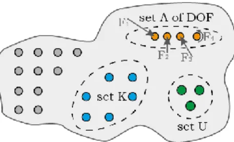
The extension of the classical displacement transmissibility has been presented in [15] and developed in [16]. In a different context, the application of the transmissibility to the force identification problem was also studied in [17-20]. A brief summary is given in what follows: we define three sets of dofs as illustrated in Fig. 1, two distinct sets U and K where the responses are measured and the set A where the
forces can be applied (and that may overlap some dofs of the other sets). Some of these forces may be zero, but the corresponding dofs have to be included in the set A.
Figure 1: Illustration of the three sets A, U and K
The responses and can be related to the applied forces through
= = U UA A K KA A Y H F Y H F (13)
where HUA is the truncated FRF matrix relating the sets of dofs U and A. Likewise, HKA relates sets K and A. Eliminating between eqs. (13), one obtains the transmissibility between and . This involves the pseudo-inverse of HKA, i.e.,
= A =
U UK K UA KA K
+
Y T Y H H Y (14)
where TUKA =HUA HKA + is the transmissibility matrix relating the displacement amplitudes of U and K for the forces at set A. This pseudo-inversion requires the size of set K to be larger or equal to the size of the set A ( ). As F has been eliminated between eqs. (13), the transmissibility depends on the A dofs A, where the forces can be applied, but not on their amplitudes; in other words, the transmissibility is invariant with respect to the amplitudes of the forces.
3.2
Methodology
The force identification consists of two steps, (i) the determination of the number and position of the forces and (ii) the evaluation of their magnitudes.
The methodology based on the transmissibility requires the knowledge of the response amplitudes YK and (the superscript“~” stands for “measured quantity”). The idea is to find the correct transmissibility matrix TUKA , that when applied to YKproduces an estimated value for that should be close enough to the measured . As the transmissibility depends on the location of the forces, one has to search for the
right set A. When the correlation between and happens, it means that the set A has been correctly found. Once again, it should be noted that the transmissibility depends only on the location of the forces (set A) but not on their amplitudes. For each possible combination of locations Ai, one has:
= Ai
U UK K
Y T Y (15)
where the index i = 1,…, refers to the number of combinations of dofs of A. The resulting is compared with the measured , using the following estimation error for each component j:
2
log log , = 1, ...length of
j j
j U U U
error =
å
Y - Y j Y (16)The accumulated error of each combination is defined as the norm of the vector = error. When this error has an absolute minimum, the correct combination of dofs Aihas been found. Naturally, the number
of loads applied to the structure is not known a priori, so we start with one force, then in combinations of two forces, etc. The number of forces that this method can find is limited by the size of the set K, as
. For a specific combination A , the reconstructed force is obtained from eq. (13) with the values i K Y , as: = i i A KA K + F H Y (17)
It is desirable that the finite element model of the original structure is updated enough, to represent as accurately as possible the experimental results of the unmodified structure.
Often, it happens that the combinations involve locations with applied forces together with locations without any force; in those situations the additional locations have zero force amplitudes and a near-zero value of accumulated error is expected. This makes the process less efficient and some kind of modification must be sought.
To avoid this issue, a modification has been introduced, consisting of computing both the reconstructed force amplitudes for every combination and the root mean square (RMS) in frequency for the forces at each dof of Ai. Whenever the accumulated error indicates a location where a load has a near-zero RMS
amplitude, its respective error is artificially increased. Such a modification improves considerably the efficiency of the force location method. Once the forces are identified, we can reconstruct the magnitude of the damage using eq. (12).
4
Numerical examples
In this section, we shall explore the possibilities of the proposed approach for detecting damage. The test item is a free rectangular plate, whose properties are given in Tab. 1; the plate is modelled using Kirchhoff-Love plate theory for finite elements with 4 nodes, each with 3 dofs (1 displacement and 2 rotations), in a 20×20 rectangular mesh. The stiffness and mass matrices are assembled and the damping is considered as negligible for the model, and of the proportional type to simulate the measurements; the proportionality is taken with respect to the stiffness matrix, with a coefficient . The code builds the dynamic stiffness matrices (with and without damping) and consequently their inverses, the FRF matrices H and H.
Five cases will be considered, (i) a loss of stiffness, (ii) a loss of mass, (iii) increase in damping, (iv) combined loss of stiffness and mass and (v) combined loss of stiffness and increase in damping.
Mass Density 7850 kg/m3
Young Elasticity Modulus 210 GPa
Thickness 1.9 mm
Width 470 mm
Height 348 mm
Table 1: Plate properties
4.1
Identification of a single force
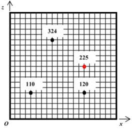
Before studying the damage cases, it is advisable to verify whether we are able to identify (localize and quantify) just the applied forces. Thus, we apply a transversal harmonic force of 1 N at node 225 of the FE model (Fig. 2), with a frequency range between 1 and 70 Hz in intervals of 1 Hz. We can compute the whole FRF matrix, but as the force is acting along the axis Oy, only the transversal displacement dofs along this direction are considered at the nodes where the displacements are “measured”.
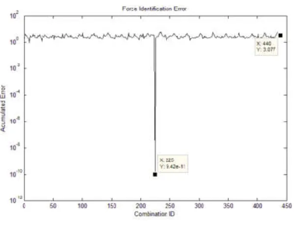
The“measured” displacements will be YK =Y120 and YU =Y324 (Y refers to the displacement along Oy and the subscript to the node), according to Fig. 2; #K = 1, therefore it is only possible to identify a single applied force. There are 441 possible locations for the force. The accumulated error (eq. (16)) for each combination is shown in Fig. 3. The minimum value of the error correctly identifies the force, at node 225. In this example the amplitude of the reconstructed force presents a maximum error of 3.7x10⁻¹⁰% . When there is no guarantee that the number of forces is just one, we can enlarge the K set, allowing the maximum number of possible locations to be 2, and looking for the combination of the force at node 225 with all the other nodes.
Any other relative minima besides the correct combination, include the correct node 225 with another location where the force presents near-zero amplitude (after reconstruction).
Figure 2: Finite element model of a plate with some representative nodes
O x 324 110 225 120 z
Figure 3: Accumulated error in frequency vs force combination for one applied force (#K=1)
4.2
Identification of a single force
4.2.1 Case 1 – Loss of stiffness
To simulate a crack, we shall consider a decrease of 10% in the stiffness at node 110. The original values of the stiffness, mass and damping at node 110 are 1.20805x10⁷ N/m, 3.32452x10⁻³kg and 1.20805x10⁻² Ns/m, respectively. Only perpendicular displacements are considered. We have considered both the cases without any noise and with some added random (normal) noise to the real and imaginary parts of the “measured” data, to simulate more realistic conditions and to test the sensitivity of the method. Two levels of noise are added: 1% and 3%.A known harmonic force with an amplitude of 1 N is applied at node 225. The unmodified model is used to identify the two forces (#A=2) using eqs. (14) and (17) and, for example,
the “measured” vectors 120, 324
T
K = Y Y
Y and YU =Y225.
The accumulated error has the minimum at the right combination (nodes 225 (applied force) and 110 (force generated by the reduced stiffness). Eq. (17) is used for the force reconstruction. The stiffness reduction is obtained from eq. (12), with a relative error of only 3.5x10⁻⁸% for -10% of damage and no added noise (Tab. 2); Y110 is calculated from eq. (15), using one of the “measured” outputs (nodes 120 or
324) and the transmissibility involving one of those output nodes and node 110, for the applied force at node 225 and no force applied at node 110. It should be stressed that we can put the force at node 110 to zero because one of the fundamental transmissibility properties is that the transmissibility is invariant with respect to the magnitude of the applied forces. This means that Y110 may be calculated (using eq. 15) from:
225 110 = 110,120 120 Y T Y (18) or 225 110 = 110,324 324 Y T Y (19)
4.2.2 Case 2 – Loss of mass
Undertaking a similar study with a variation in the mass, again at node 110, considering once more a decrease of 10%, we obtained the results shown in (Tab. 3). The same “measured” vectors
120, 324
T
K = Y Y
Damage (%) Imposed K [N/m] Added noise level (%) Localization Identified K [N/m] Relative error (%) -10 -1.20805E+06
0 Y (node 110) -1.20805E+06 3.50E-08
1 Y (node 110) -1.76911E+06 4.64E+01
3 N (node 187) ---
---Table 2:Identification of a loss of stiffness
Damage (%) Imposed M [kg] Added noise level (%) Localization Identified M [N/m] Relative error (%) -10 -3.324500E-04
0 Y (node 110) -3.324500E-04 7.90E-05
1 N (node 189) ---
---3 N (node 165) ---
---Table 3: Identification of a loss of mass
4.2.3 Case 3– Increase of damping
Here we impose an increase of ten times (1000%) in the damping, again at node 110. The results are given in (Tab. 4), always using the “measured” vectors 120, 324
T K = Y Y Y and YU =Y225. Damage (%) Imposed C [Ns/m] Added noise level (%) Localization Identified C [Ns/m] Relative error (%) +1000 +1.20805E-01
0 Y (node 110) +1.20226E-01 4.80E-01
1 Y (node 110) +2.67367E-01 1.21E+02
3 N (node 109) ---
---Table 4: Identification of an increase in damping
4.2.4 Case 4– Simultaneous loss of stiffness and mass
Here, we introduced a variation of 10% in both the stiffness and mass in node 110. The results are presented in Tab. 5, using the “measured” vectors YK = Y120,Y324 Tand .
Damage (%) Imposed K [N/m] and M [kg] Added noise level (%) Localization Identified K [N/m] and M [kg] Relative error (%) -10 -1.20805E+06 -3.324500E-04 0 Y (node 110) -1.20805E+06 -3.324642E-04 6.30E-08 4.27E-03 1 Y (node 110) -1.75934E+06 -1.23978E+01 4.56E+01 --3 Y (node 110) -1.36993E+06 -4.65631E+00 1.34E+01 --Table 5: Identification of a loss of stiffness and mass
4.2.5 Case 5– Simultaneous loss of stiffness and increase in damping
Now, we introduce a decrease of 10% in the stiffness and a 1000% increase in the damping, always at
node 110 and for the same “measured” vectors 120, 324
T
K = Y Y
Y and . The results are presented in
Tab. 6. Damage (%) Imposed K [N/m] and C [Ns/m] Added noise level (%) Localization Identified K [N/m] and C [Ns/m] Relative error (%) -10 in K +1000 in C -1.20805E+06 +1.20805E-01 0 Y (node 110) -1.20805E+06 0.82239E-02 6.30E-08 9.32E+01 1 Y (node 110) -2.84822E+06 +7.6455E-02 1.36E+02 3.67E+01 3 Y (node 165) ---
---Table 6: Identification of a loss of stiffness and increase in damping
5
Discussion
The results of these numerical simulations without added noise show that in almost all the situations the localization of the damage is achieved with good accuracy; When the data is “perfect”, i.e., without any added noise, the quantification of damage is always correct, except when the change in the damping is considered. When noise is added to the “measured” responses, the results show a very high sensitivity of the method to this parameter, as it is common in such inverse problems. Up to 1% of added random noise the localization of the damage still worked well in most cases. However, the quantification of the damage
exhibited very high errors, as the noise strongly affects the reconstruction of the forces. The stiffness is the property that better “resists” to the existence of noise in the data, namely for the localization step. The most sensitive is the damping.
These results still have space for some improvements. Note that none of the known tools to deal with noisy signals have been used in this work; the authors will be addressing this in future work.
6
Conclusions
It has been shown that it is possible to establish a relation between the identification of damage and the identification of dynamic forces. While the damage is modeled through the variation of the structure properties (mass, stiffness and damping), the force identification is accomplished by a methodology that uses the displacement transmissibility between groups of coordinates. Whenever a damage occurs, new forces directly related to the changes in the dynamic properties appear and those additional forces are then identified using the transmissibility.
In principle, and in the context of damage identification, the procedure seems potentially suitable for the detection, localization and also quantification of a structural modification, or even more than one. The results without any added noise illustrate the effectiveness of the method. The simulations with added random noise up to 1% and damages of 10% in the stiffness and mass and 1000% in the damping show that the method works reasonably well in the detection and localization steps concerning changes only in the stiffness, but fails in the quantification, mainly when it comes to damages due to mass and damping variations. Although not shown in this work, the choice of different frequency ranges does not seem to have a significant effect on the results, something that was not anticipated initially. Further research from both the numerical and experimental points of view will be necessary to improve the procedure.
Acknowledgements
The authors thank the Portuguese Science Foundation, FCT, through IDMEC, under LAETA, project no. UID/EMS/50022/2013 and under the project UNIDEMI Pest-OE/EME/UI0667/2014.
References
[1] Mas, P., Sas, P., Indirect force identification based on impedance matrix inversion: a study on statistical and deterministic accuracy, Proceedings of 19th ISMA, (1994), pp. 1049-1065.
[2] Dobson, B. J., Rider, E., A review of the indirect calculation of excitation forces from measured structural response data, J. of Mechanical Engineering Science , 204(2), (1990), pp. 69-75.
[3] Tao, J. S., Liu, G. R., Lam, K. Y., Excitation Force Identification of an Engine with Velocity Data at Mounting Points, J. of Sound and Vibration, 242(2), (2001), pp. 321-331.
[4] Uhl, T., The inverse identification problem and its technical application, Archive of Applied Mechanics, 77(5), (2007), pp. 325-337.
[5] McColl, C., Palmer, D., Chierichetti, M., Bauchau, O., Ruzzene, M., Comprehensive UH-60 loads model validation, Proceedings of 66th Annual Forum - American Helicopter Society, (2010), pp. 1531-156.
[6] Vyas, N. S., Wicks, A. L., Reconstruction of turbine blade forces from response data, Mechanism and Machine Theory, 36, (2001), pp. 177-188.
[7] Lage, Y. E., Maia, N. M. M., Neves, M. M., Ribeiro, A.M.R., A Force Identification Approach for Multiple-Degree-of-Freedom Systems, Proceedings of IMAC-XXVIII, (2010), pp. 53-61.
[8] Ma, C. K., Ho, C. C., An inverse method for the estimation of input forces acting on non-linear structural systems, Journal of Sound and Vibration, 275, (2004), pp. 953-971.
[9] Choi, H. G., Thite, A. N., Thompson, D. J., A threshold for the use of Tikhnov regularization in inverse force determination, Applied Acoustics, 67, (2006), pp. 700-719.
[10] Thite, A. N., Thompson, D. J., The quantification of structure-borne transmission paths by inverse methods. Part1: improved singular value rejection methods, Journal of Sound and Vibration, 264, (2003), pp. 411-431.
[11] Thite, A. N., Thompson, D. J., The quantification of structure-borne transmission paths by inverse methods. Part 2: use of regularization methods, Journal of Sound and Vibration, 264, (2003), pp. 433-451.
[12] Chang, C., Sachse, W., Analysis of elastic wave signals from an extended source in a plate," Journal of the Acoustical Society of America, 77(4), (1985), pp. 1335-1341.
[13] Michaels, J. E., Pao, Y.-H., The inverse source problem for an oblique force on an elastic plate," Journal of the Acoustical Society of America, 77(6), (1985), pp. 2005–2011.
[14] D'Cruz, J., Crisp, J. D. C., Ryall, T. G., On the Identification of a harmonic force on a viscoelastic plate from response data, Journal of Applied Mechanics, 59, (1992), pp. 722-729.
[15] Maia, N. M. M., Silva, J. M. M., Ribeiro, A. M. R., The transmissibility concept in multi-degree-of-freedom systems, Mechanical Systems and Signal Processing, 15 (1), (2001), pp.129-137.
[16] Maia, N. M. M., Urgueira, A. P. V., Almeida, R. A. B., Whys and wherefores of transmissibility, in Vibration Analysis and Control - New Trends and Developments, Dr. Francisco Beltran-Barbajal, InTech, (2011), pp. 197-216.
[17] Lage, Y. E., Maia, N. M. M., Neves, M. M., Ribeiro, A. M. R., Force identification using the concept displacement transmissibility, Journal of Sound and Vibration, 332(7), (2013), pp. 1674-1686.
[18] Neves, M. M., Maia, N. M. M., Estimation of applied forces using the transmissibility concept, Proceedings of ISMA2010, (2010), pp. 3887-3897.
[19] Maia, N. M. M., Lage, Y. E., Neves, M. M., Recent advances on force identification in structural dynamics, in Advances in Vibration Engineering and Structural Dynamics, InTech, (2012), pp. 103-132.
[20] Lage, Y. E., Neves, M. M., Maia, N. M. M., Tcherniak, D., Force transmissibility versus displacement transmissibility, Journal of Sound and Vibration, 333(22), (2014), pp. 5708-5722.