DAMAGE LOCALIZATION IN LAMINATED COMPOSITE PLATES USING DOUBLE PULSE-ELECTRONIC HOLOGRAPHIC INTERFEROMETRY

Lisbon, Portugal, 5–8 June 2006

DAMAGE LOCALIZATION IN LAMINATED COMPOSITE PLATES

USING DOUBLE PULSE-ELECTRONIC HOLOGRAPHIC

INTERFEROMETRY

J.V. Ara ´ujo dos Santos1

, H.M.R. Lopes2

, M. Vaz3

, C.M. Mota Soares1

, C.A. Mota Soares1

, and M.J.M. de Freitas4

1

IDMEC/IST, Instituto Superior T´ecnico Av. Rovisco Pais, 1049-001 Lisboa, Portugal

jsantos@dem.ist.utl.pt cmmsoares@alfa.ist.utl.pt carlosmotasoares@dem.ist.utl.pt

2

ESTIG - Instituto Polit´ecnico de Braganc¸a

Campus de Sta Apol´onia, Apartado 134, 5301-857 Braganc¸a, Portugal hlopes@ipb.pt

3

DEMEGI - Faculdade de Engenharia do Porto Rua Dr. Roberto Frias, 4200-465 Porto, Portugal

gmavaz@fe.up.pt

4

ICEMS/UME, Instituto Superior T´ecnico Av. Rovisco Pais, 1049-001 Lisboa, Portugal

mfreitas@dem.ist.utl.pt

Keywords: Damage Localization, Laminated Plate, Mode Shape Curvature, Double Pulse-Electronic Holographic Interferometry, Acoustic Excitation, Non Destructive Inspection.

1 INTRODUCTION

In recent years the use of laminated composite materials in many mechanical and aerospace engineering structures has seen a huge increase, due, among other factors, to their specific stiff-ness and strength. However, because of these materials characteristics, damage can be produced during fabrication or by inappropriate or hazardous service loads. Delamination is one the most common and dangerous damages, caused by internal failure of the laminas interface. These internal damages can be undetected by visual inspection. Therefore, in order to assess the struc-ture integrity, non destructive inspection methods are needed for damage localization. The most used non destructive inspection methods are either visual or localized experimental methods such as acoustic or ultrasonic methods, magnet field methods, radiographs, eddy-current meth-ods and thermal field methmeth-ods [1]. These experimental methmeth-ods can detect damage on or near the surface of the structure [1], therefore not allowing the detection of delaminations.

The use of vibration based delamination identification and health monitoring techniques for

composite structures have been surveyed by Zouet al. [2]. The level of success in identifying

damage is directly related to the sensitivity of the applied measurement technique and the pa-rameters used in the identification methodology. Abdo and Hori [3], showed numerically that damage localization by mode shapes can be more easily accomplished if rotation differences are involved. However, in the presence of small defects with noisy data, obtained from experi-mental measurement, the use of rotations can mislead the damage localization. In these cases, a higher sensitivity parameter, like the curvature or strain energy, could be used instead [4, 5].

One method for the damage localization of impact damage in laminated composite plates, based on mode shapes curvature differences, is presented, applied and discussed in this paper. The measurement of mode shapes translations is performed using double pulse-electronic holo-graphic interferometry and the plate is excited acoustically. In order to overcome the problem of differentiating noisy data, the rotations and curvatures are obtained by numerical differentiation of modes shapes translations using a differentiation/smoothing technique [6, 7, 8, 9, 10, 11].

The proposed methodology was applied to a carbon fiber reinforced epoxy rectangular plate, free in space, subjected to two cases of impact damage. The results of applying the mentioned method showed that the curvature differences allow the localization of both cases of damage, which can be undetected by visual, standard X-ray or C-Scan inspections. Finally, it was also found that the best localizations are achieved by selecting the most changed mode, due to the presence of damage.

2 EXPERIMENTAL SETUP

A carbon fiber reinforced epoxy rectangular plate, with a [0/90/+45/−45/0/90]s stacking

sequence, was analyzed before and after being damaged by impact using the experimental

tech-niques described in this Section. The plate in-plane dimensions are277.0mm×199.0mm and

its thickness is 1.80 mm. The specific mass is ρ = 1562kg/m3

and the laminas mechanical

properties are E1 = 123.4 GPa, E2 = 8.6 GPa, G12 = G13 = 5.0 GPa, G23 = 6.1 GPa,

ν12 = 0.14, which were obtained using a technique described in [12]. The first ten natural

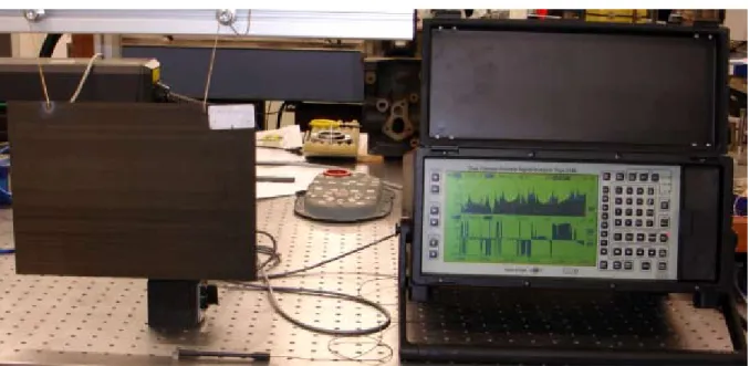
fre-quencies of the plate were obtained from its Frequency Response Functions (FRFs). The plate was suspended with high flexible rubber bands creating a nearly free condition. A transient

excitation was performed with an impact hammer Br¨uel & Kjær model 8203 and a non

con-tact measurement of the plate response was carried out with a microphone. Both signals were

processed in aBr¨uel & Kjær analyzer, model 2148. In Figure 1 is shown a view of the setup

Figure 1: Experimental setup for Frequency Response Functions measurements.

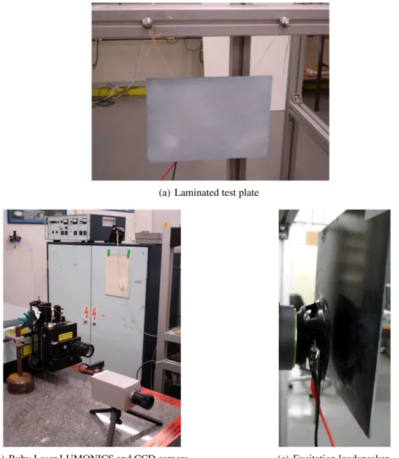
A double pulse-electronic holographic interferometry set up with acoustic excitation was used to assess the plate mode shapes. This high sensitive technique allows a non contact mea-surement of the mode shapes with no influence in the plate mass distribution. A double-pulsed

Ruby Laser was used to generate pairs of pulses with a time separation varying between 1µs and

800µs. The double pulse speckle patterns were recorded with an asynchronous CCD camera,

with a 512×512 resolution (Figures 2 and 3).

PC Signal generator

Trigger system

Trigger signal

Laser control

Double pulse Ruby laser Illumination

device

Plate

Video signal

Camera

Loudspeaker

Figure 2: Schematic of experimental setup for mode shapes measurements.

To assess the phase map of each speckle pattern a spatial carrier is introduced in the primary fringes by a small tilt in the reference wave front [13]. Due to the short time between recordings, any low frequency rigid body movement of the plate is eliminated. The two interferograms are post-processed using dedicated image processing techniques [7, 10, 11, 14, 15, 16, 17, 18, 19] and thus the mode shapes translations are obtained.

(a) Laminated test plate

(b) Ruby Laser LUMONICS and CCD camera (c) Excitation loudspeaker

Figure 3: Experimental setup for mode shapes measurements.

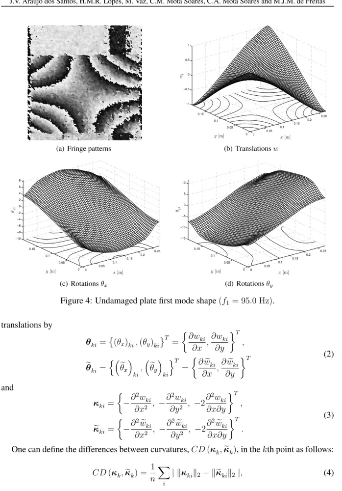
Between each evaluation a smoothing algorithm is applied [7]. Figures 4 and 5 show the un-damaged plate fringe patterns, translations and rotations of the first and tenth mode shapes, respectively.

3 DAMAGE LOCALIZATION METHOD

Consider thekth point, with(x, y)coordinates, and theith mode shape of a plate. Let their

undamaged and damaged out-of-plane translations be defined as

wki and weki. (1)

(a) Fringe patterns 0 0.05 0.1 0.15 0.2 0.25 0 0.05 0.1 0.15 −1 −0.5 0 0.5 1 x[m] y[m] w1

(b) Translationsw

0 0.05 0.1 0.15 0.2 0.25 0 0.05 0.1 0.15 −10 −8 −6 −4 −2 0 2 4 6 8 x[m] y[m]

θx1

(c) Rotationsθ

x 0 0.05 0.1 0.15 0.2 0.25 0 0.05 0.1 0.15 −15 −10 −5 0 5 10 x[m] y[m]

θy1

(d) Rotationsθ

y

Figure 4: Undamaged plate first mode shape(f1 = 95.0 Hz).

translations by

θ

ki =

(θx)_ki,(θy)_ki T = ∂w_ki ∂x , ∂w_ki ∂y T , e

θ_{ki =}

n e

θ_x

ki

,θe_y

ki oT

=

∂w_eki

∂x ,

∂w_eki ∂y

T (2)

and

κ_{ki =}

−∂

2

w_ki

∂x2 , −

∂2

w_ki

∂y2 , −2

∂2 w_ki ∂x∂y T , e κ ki = −∂ 2 e w_ki

∂x2 , −

∂2

e w_ki

∂y2 , −2

∂2 e w_ki ∂x∂y T . (3)

One can define the differences between curvatures,CD(κ

k,κek), in thekth point as follows:

CD(κ

k,κek) =

1

n X

i | kκ

kik2− kκe_kik2 |, (4)

wherekκ

kik2,kκe_kik2are the Euclidean norms of vectorsκ_kiandκe_ki, respectively. The number

(a) Fringe patterns

0 0.05

0.1 0.15

0.2 0.25

0 0.05 0.1 0.15 −1 −0.5 0 0.5 1

x[m] y[m]

w1

0

(b) Translationsw

0 0.05

0.1 0.15

0.2 0.25

0 0.05 0.1 0.15 −30 −25 −20 −15 −10 −5 0 5 10 15

x[m] y[m]

θx1

0

(c) Rotationsθ

x

0 0.05

0.1 0.15

0.2 0.25

0 0.05 0.1 0.15 −30 −20 −10 0 10 20

x[m] y[m]

θy1

0

(d) Rotationsθ

y

Figure 5: Undamaged plate tenth mode shape(f10 = 770.5 Hz).

chosen mode shape included in the computation ofCD(κ

k,κek). In what follows, the method

defined by expression (4) will be referred as Curvature Differences method.

4 APPLICATIONS

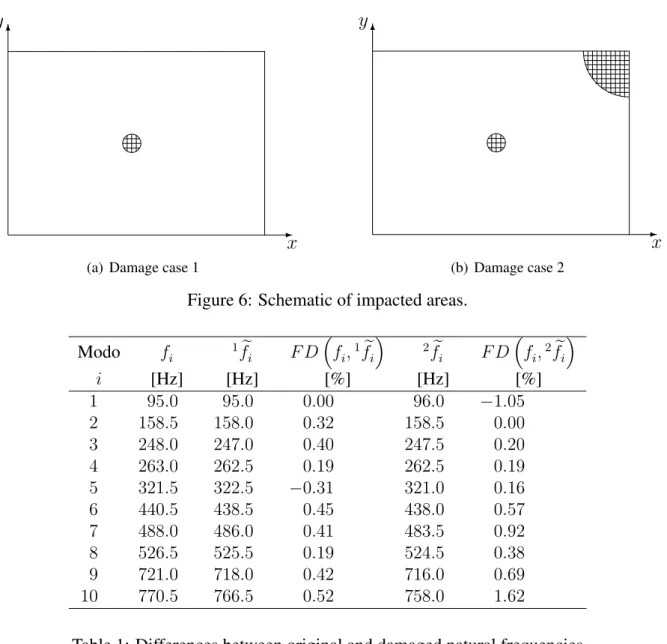
The plate presented in Section 2 was subjected to two cases of damage. The first case cor-responds to a damage generated by a low energy impact in the center of the plate (Figure 6(a)), by dropping a steel ball. After measuring the natural frequencies and mode shapes, using the procedures described in Section 2, a second damaged was introduced in the plate by percuting the plate right upper corner (Figure 6(b)) with a rounded steel tip hammer and again the natural frequencies and mode shapes were measured.

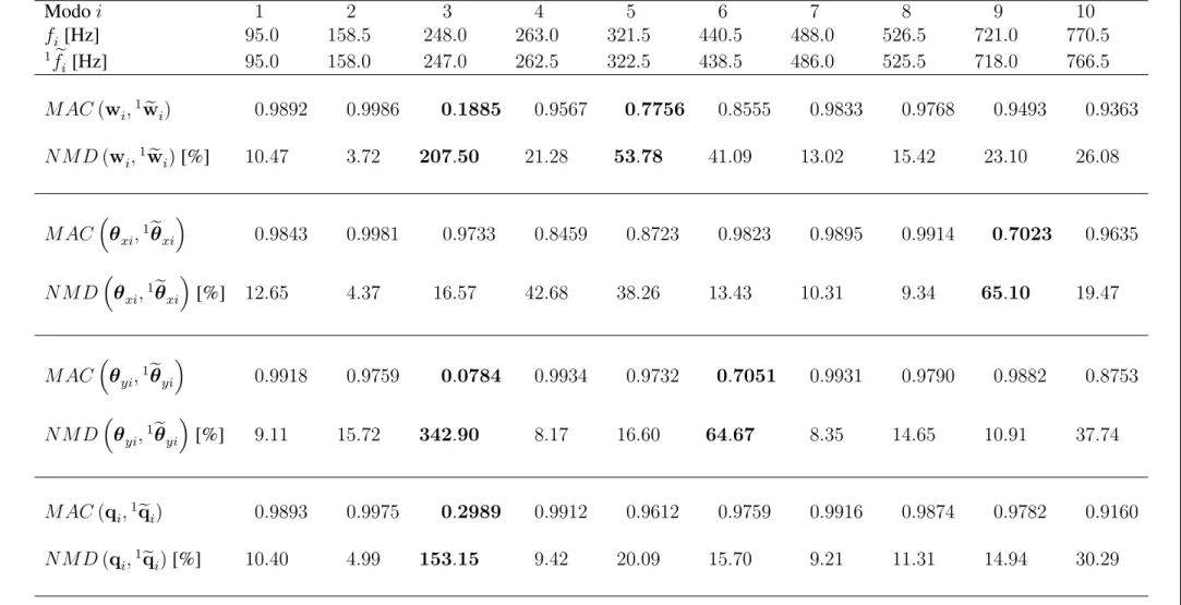
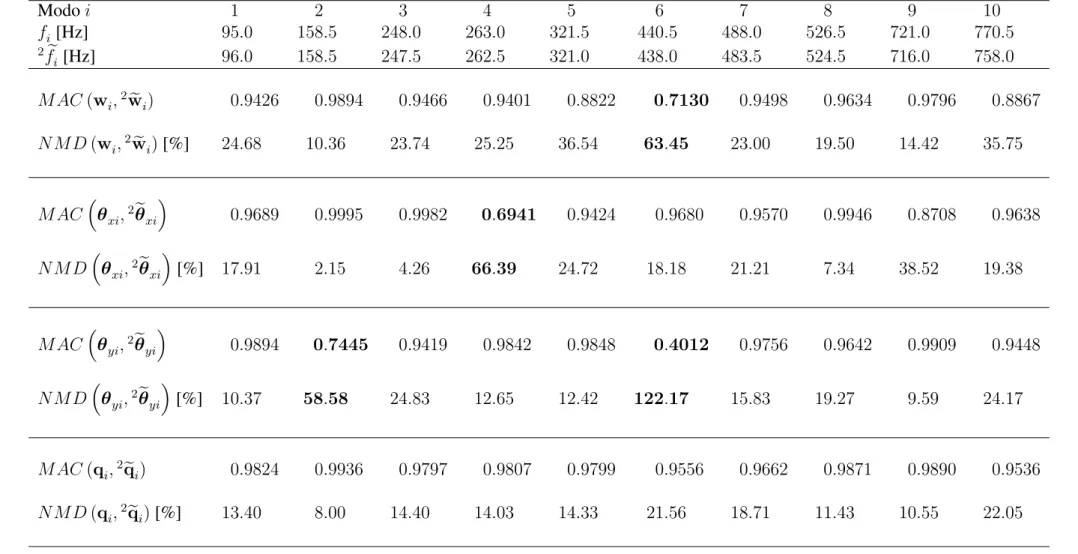
Table 1 presents the percentual differences between the natural frequencies in the undamaged state (original natural frequencies) and the natural frequencies for both cases of damage (dam-aged natural frequencies). The numerical superscripts in Table 1 denote the case of damage and

the values ofF Dare given by

F Df_i,1fe_i= fi−

1e

f_i

f_i ×100 and F D

f_i,2fe_i= fi−

2e

f_i

f_i ×100.

Crite-✲ ✻

x

y

(a) Damage case 1

✲ ✻

x

y

(b) Damage case 2

Figure 6: Schematic of impacted areas.

Modo f_i 1e

f_i F Df_i,1e

f_i 2e

f_i F Df_i,2e

f_i

i [Hz] [Hz] [%] [Hz] [%]

1 95.0 95.0 0.00 96.0 −1.05

2 158.5 158.0 0.32 158.5 0.00

3 248.0 247.0 0.40 247.5 0.20

4 263.0 262.5 0.19 262.5 0.19

5 321.5 322.5 −0.31 321.0 0.16

6 440.5 438.5 0.45 438.0 0.57

7 488.0 486.0 0.41 483.5 0.92

8 526.5 525.5 0.19 524.5 0.38

9 721.0 718.0 0.42 716.0 0.69

10 770.5 766.5 0.52 758.0 1.62

Table 1: Differences between original and damaged natural frequencies

rion (MAC) and the Normalized Modal Difference (NMD) parameters defined by

M AC(w_i,w_ei) =

(w_i)T (w_ei) 2

h

(w_i)T (w_i)i h(we_i)T (we_i)i

for 0< M AC(w_i,w_ei)61,

N M D(w_i,w_ei) =

s

1−M AC(w_i,w_ei)

M ACθ

xi,eθxi = (θ xi) T _eθ

xi 2 h (θ xi) T (θ xi) i e θ xi T e θ xi

for 0< M AC

θ

xi,eθxi

61,

N M Dθ_xi,eθ_xi

= v u u u t

1−M ACθ

xi,eθxi

M ACθ

xi,eθxi

for 06N M Dθ_xi,eθ_xi

<∞;

M ACθ

yi,θeyi = θ yi

T_e

θ yi 2 h θ yi T θ yi

i_e

θ yi T e θ yi

for 0< M AC

θ

yi,eθyi

61,

N M Dθ

yi,θeyi = v u u u

t1−

M ACθ_yi,eθ_yi

M ACθ

yi,θeyi

for 06N M Dθ

yi,eθyi

<∞;

M AC(q_i,_eq_i) =

(q_i)T (eq_i) 2

h

(q_i)T (q_i)i h(_eq_i)T (_eq_i)i

for 0< M AC(q_i,q_ei)61,

N M D(q_i,_eq_i) =

s

1−M AC(q_i,_eq_i)

M AC(q_i,_eq_i) for 06N M D(qi,eqi)<∞,

where w_i e w_ei, θ

xi and eθxi, θyi and θeyi are, respectively, the partition vectors of the global

vectorsq_i = w_i,θ_xi,θ_{yi andeqi =} n_wei,eθ_xi,θe_yio_{, relative to the translations and rotations}

aboutyandxaxis, of theith mode.

The values ofM ACandN M D, presented in Tables 2 and 3, were obtained taking into

ac-count481components in the partition vectors and1443components in vectorsq_i e_eq_i.

There-fore, these vectors contain the translations and rotations in481points, schematically represented

by black dots in Figure 7. The choice of these points was made in order to compare the experi-mental mode shapes with those numerically obtained, using a plate finite element model based

on the first order shear deformation theory [12]. In Tables 2 and 3, the values ofN M D greater

than50%and the correspondingM ACare printed in bold.

Figure 7: Distribution of points for the computation ofM ACandN M D.

0 0.05

0.1 0.15

0.2 0.25

0 0.05 0.1 0.15 −1 −0.5 0 0.5 1

x[m] y[m]

w3

(a) Undamaged

0 0.05

0.1 0.15

0.2 0.25

0 0.05 0.1 0.15 −1 −0.8 −0.6 −0.4 −0.2 0 0.2 0.4 0.6 0.8

x[m] y[m]

1ew

3

(b) Damage case 1

Figure 8: Third mode shape translations.

0 0.05

0.1 0.15

0.2 0.25

0 0.05 0.1 0.15 −1 −0.5 0 0.5 1

x[m] y[m]

w6

(a) Undamaged

0 0.05

0.1 0.15

0.2 0.25

0 0.05 0.1 0.15 −1 −0.5 0 0.5 1

x[m] y[m]

2ew

6

(b) Damage case 2

.

Ara

´ujo

dos

Santos,

H.M.R.

Lope

s,

M.

V

az,

C.M.

Mota

Soares,

C.A.

Mota

Soares

and

M.J.M

.

de

Freitas

Modoi 1 2 3 4 5 6 7 8 9 10

f_i [Hz] 95.0 158.5 248.0 263.0 321.5 440.5 488.0 526.5 721.0 770.5

1e

f_i [Hz] 95.0 158.0 247.0 262.5 322.5 438.5 486.0 525.5 718.0 766.5

M AC(w_i,1

e

w_i) 0.9892 0.9986 0.1885 0.9567 0.7756 0.8555 0.9833 0.9768 0.9493 0.9363

N M D(w_i,1

e

w_i)[%] 10.47 3.72 207.50 21.28 53.78 41.09 13.02 15.42 23.10 26.08

M ACθ

xi,

1e_θ

xi

0.9843 0.9981 0.9733 0.8459 0.8723 0.9823 0.9895 0.9914 0.7023 0.9635

N M Dθ

xi,

1e_θ

xi

[%] 12.65 4.37 16.57 42.68 38.26 13.43 10.31 9.34 65.10 19.47

M ACθ

yi,

1e_θ

yi

0.9918 0.9759 0.0784 0.9934 0.9732 0.7051 0.9931 0.9790 0.9882 0.8753

N M Dθ

yi,

1e_θ

yi

[%] 9.11 15.72 342.90 8.17 16.60 64.67 8.35 14.65 10.91 37.74

M AC(q_i,1

e

q_i) 0.9893 0.9975 0.2989 0.9912 0.9612 0.9759 0.9916 0.9874 0.9782 0.9160

N M D(q_i,1

e

q_i)[%] 10.40 4.99 153.15 9.42 20.09 15.70 9.21 11.31 14.94 30.29

Table 2: Differences between original and damaged mode shapes (Damage case 1)

´ujo

dos

Santos,

H.M.R.

Lope

s,

M.

V

az,

C.M.

Mota

Soares,

C.A.

Mota

Soares

and

M.J.M

.

de

Freitas

Modoi 1 2 3 4 5 6 7 8 9 10

f_i [Hz] 95.0 158.5 248.0 263.0 321.5 440.5 488.0 526.5 721.0 770.5

2e

f_i [Hz] 96.0 158.5 247.5 262.5 321.0 438.0 483.5 524.5 716.0 758.0

M AC(w_i,2

e

w_i) 0.9426 0.9894 0.9466 0.9401 0.8822 0.7130 0.9498 0.9634 0.9796 0.8867

N M D(w_i,2

e

w_i)[%] 24.68 10.36 23.74 25.25 36.54 63.45 23.00 19.50 14.42 35.75

M ACθ

xi,

2e_θ

xi

0.9689 0.9995 0.9982 0.6941 0.9424 0.9680 0.9570 0.9946 0.8708 0.9638

N M Dθ

xi,

2e_θ

xi

[%] 17.91 2.15 4.26 66.39 24.72 18.18 21.21 7.34 38.52 19.38

M ACθ

yi,

2e_θ

yi

0.9894 0.7445 0.9419 0.9842 0.9848 0.4012 0.9756 0.9642 0.9909 0.9448

N M Dθ

yi,

2e_θ

yi

[%] 10.37 58.58 24.83 12.65 12.42 122.17 15.83 19.27 9.59 24.17

M AC(q_i,2

e

q_i) 0.9824 0.9936 0.9797 0.9807 0.9799 0.9556 0.9662 0.9871 0.9890 0.9536

N M D(q_i,2

e

q_i)[%] 13.40 8.00 14.40 14.03 14.33 21.56 18.71 11.43 10.55 22.05

Table 3: Differences between original and damaged mode shapes (Damage case 2)

4.1 Proposed non destructive inspection methods

Damage localization using 10 mode shapes

The following damage localizations results were obtained using the first ten mode shapes,

i.e., consideringn= 10andi= 1, ...,10in expression (4).

By applying the Curvature Differences method, one can see that the greatest values of

CD(κ

k,κek) appear in the right upper corner of the plate (Figure 10(b)), while the damage

in the plate center is not located (Figure 10(a)).

0 0.05 0.1 0.15 0.2 0.25 0 0.05 0.1 0.15 10 20 30 40 50 60 70 x[m] y[m] 1C D ( κ k ,

eκk

)

(a) Damage case 1

0 0.05 0.1 0.15 0.2 0.25 0 0.05 0.1 0.15 10 20 30 40 50 60 70 80 90 100 x[m] y[m] 2C D ( κk , eκ k )

(b) Damage case 2

Figure 10: Damage localization with Curvature Differences method and 10 modes.

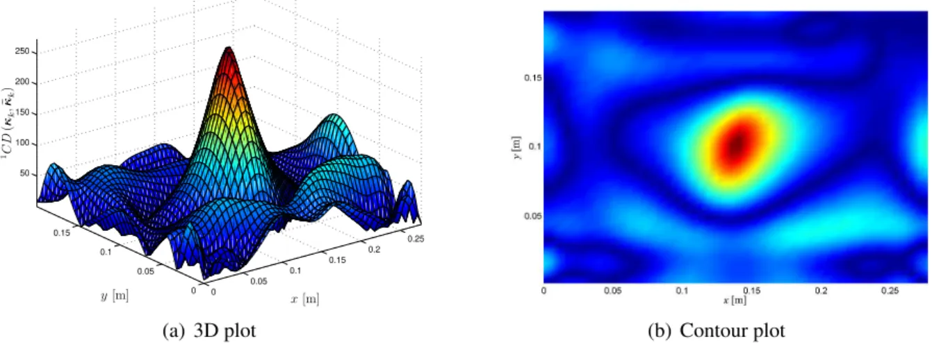
Damage localization using the most changed mode shape

Figures 11(a) and 11(b) present, respectively, a 3D plot and a contour plot of CD(κ

k,κek)

values obtained by applying the Curvature Differences method to the most change mode shape,

due to the damage in the plate center,i.e., the third mode shape (see Table 2), by definingn = 1

and i = 3 in expression (4). The corresponding undamaged and damage natural frequencies

are, respectively,f3 = 248Hz and

1e

f3 = 247Hz. It can be undoubtedly seen that the damage

is located. 0 0.05 0.1 0.15 0.2 0.25 0 0.05 0.1 0.15 50 100 150 200 250 x[m] y[m] 1C D ( κk , e κk )

(a) 3D plot (b) Contour plot

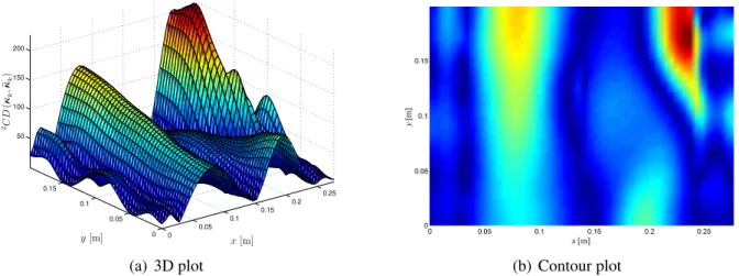
For both damages, one in the plate center and the other on its upper right corner, the most changed mode is the sixth (see Table 3), to which correspond the undamaged and damage

natural frequenciesf3 = 440.5Hz and

2e

f6 = 438.0Hz, respectively. The Curvature Differences

method results, using only this mode shape curvature (n = 1andi = 6in expression (4)) are

presented in a 3D plot and a contour plot in Figures 12(a) and 12(b). These Figures show the presence of damage in the plate upper right corner. However, the damage present in the plate center is not detected.

0 0.05

0.1 0.15

0.2 0.25

0 0.05 0.1 0.15 50 100 150 200

x[m] y[m]

2C

D

(

κ

k

,

e

κk

)

(a) 3D plot (b) Contour plot

Figure 12: Damage case 2 localization with Curvature Differences method and sixth mode (f6 = 440.5Hz).

4.2 Other non destructive inspection methods

The damages inflicted to the plate are not detected by global visual inspection. Only by close examination is it possible to see some small indentations on the plate surface, where the impacts were made. The presence of damages was also not detected by standard X-ray inspections.

After both damages were inflicted to the plate, a C-Scan analysis was also performed. Fig-ures 13(a) and 13(b) present the scanning results for all plate and for its center area, respectively. One notes that the damage in the center of the plate is detected, although the damage in the plate upper right corner is not. Since the damage in this area was inflicted by percussion with a ham-mer, the S-Can is unable to detect it.

5 CONCLUSIONS

(a) C-scan of all plate (b) C-scan of plate center

Figure 13: C-Scan of plate with damage in center and upper right corner.

ACKNOWLEDGEMENTS

The authors greatly appreciate the financial support of FCT/POCTI/FEDER, FCT/POCTI (2010)/FEDER, Project POCTI/EME/56616/2004 and the EU through FP6-STREP Project Con-tract No. 013517-NMP3-CT-2005-0135717. The first author is most obliged to Prof. Lu´ıs Reis for preparing the laminated plate and to Mr. Manuel Bessa for performing the X-ray analysis.

REFERENCES

[1] S.W. Doebling, C.R. Farrar, M.B. Prime and D.W. Shevitz. Damage identification and

health monitoring of structural and mechanical systems from changes in their vibration characteristics: A literature review. LA–13070–MS, Los Alamos National Laboratory, 1996.

[2] Y. Zou, L. Tong and G.P. Steven. Vibration-based model-dependent damage

(delamina-tion) identification and health monitoring for composites structures - a review,Journal of

Sound and Vibration,230(2), 357–378, 2000.

[3] M.A.-B. Abdo and M. Hori. A numerical study of structural damage detection using

changes in the rotation of mode shapes, Journal of Sound and Vibration, 251(2), 227–

239, 2002.

[4] A.K. Pandey, M. Biswas and M.M. Samman. Damage detection from changes in curvature

mode shapes,Journal of Sound and Vibration,145(2), 321–332, 1991.

[5] E. Sazonov and P. Klinkhachorn. Optimal spatial sampling interval for damage detection

by curvature or strain energy mode shapes, Journal of Sound and Vibration, 285(4–5),

783–801, 2005.

[6] C. Reinsch C. This week’s citation classic: Reinsch C H, smoothing by spline functions,

Current Contents/Engineering Technology & Applied Sciences,24, 20, 1982.

[7] H.M.R. Lopes, R.M. Guedes and M.A. Vaz. An improved mixed numerical-experimental

method for stress field calculation.Optics & Laser Technology, 2005 (Accepted for

[8] J. Babaud, A.P. Witkin, M. Baudin and R.O. Duda. Uniqueness of the gaussian kernel for

scale-space filtering, IEEE Transactions on Pattern Analysis and Machine Intelligence,

8(1), 26–33, 1986.

[9] J. Bevington and M. Mersereau. Diferential operator based edge and line detection, In: IEEE International Conference on ICASSP ’87, Vol. 7, 249–252, 1987.

[10] C.A. Sciammarella and T.Y. Chang. Holographic interferometry applied to the solution of

a shell problem,Experimental Mechanics,14(6), 217–224, 1974.

[11] C.A. Sciammarella and S.K. Chawla. Lens holographic-moire technique to obtain

compo-nents of displacements and derivatives,Experimental Mechanics,18(10), 373–381, 1978.

[12] C.M.M. Mota Soares, M.M. Freitas, A.L. Ara´ujo and P. Pedersen. Identification of

ma-terial properties of composite plate specimens,Composite Structures, 25(1–4), 277–285,

1993.

[13] M. Takeda, H. Ina and S. Kobayashi. Fourier-transform method of fringe-pattern

analy-sis for computer-based topography and interferometry,Journal of the Optical Society of

America,72(1), 156–160, 1982.

[14] J.A.G. Chousal.T´ecnicas de processamento de imagens obtidas por m´etodos ´opticos em

an´alise experimental de tens˜oes, Ph.D. thesis, Faculdade de Engenharia da Universidade do Porto, Departamento de Engenharia Mecˆanica e Gest˜ao Industrial, Porto, 1999 (In Portuguese).

[15] D.C. Ghiglia and M.D. Pritt. Two-Dimensional Phase Unwrapping: Theory, Algorithms, and Software, Wiley, New York, , Chap. xiv, p. 493, 1998.

[16] Q. Kemao. Windowed fourier transform for fringe pattern analysis, Applied Optics,

43(13), 2695–2702, 2004.

[17] Q. Kemao. Windowed fourier transform for fringe pattern analysis: Addendum, Applied

Optics,43(17), 3472–3473, 2004.

[18] G. Pedrini, B. Pfister and H. Tiziani. Double pulse-electronic speckle interferometry,

Jour-nal of Modern Optics,40(1), 89–96, 1993.

[19] V.V. Volkov and Y.M. Zhu. Deterministic phase unwrapping in the presence of noise,