Energy prices forecasting using GLM

Repositório ISCTE-IUL

Deposited in Repositório ISCTE-IUL:

Deposited version:

Peer-review status of attached file:

Citation for published item:

Teodoro, M. F., Andrade, M., Silva, E. C., Borges, A. & Covas, R. (2018). Energy prices forecasting using GLM. In Teresa A. Oliveira, Christos P. Kitsos, Amílcar Oliveira, Luís Grilo (Ed.), Recent studies in risk analysis and statistical modeling.: Springer.

Further information on publisher's website:

Publisher's copyright statement:

This is the peer reviewed version of the following article: Teodoro, M. F., Andrade, M., Silva, E. C., Borges, A. & Covas, R. (2018). Energy prices forecasting using GLM. In Teresa A. Oliveira, Christos P. Kitsos, Amílcar Oliveira, Luís Grilo (Ed.), Recent studies in risk analysis and statistical modeling.: Springer.. This article may be used for non-commercial purposes in accordance with the Publisher's Terms and Conditions for self-archiving.

Use policy

Creative Commons CC BY 4.0

The full-text may be used and/or reproduced, and given to third parties in any format or medium, without prior permission or charge, for personal research or study, educational, or not-for-profit purposes provided that:

• a full bibliographic reference is made to the original source • a link is made to the metadata record in the Repository • the full-text is not changed in any way

The full-text must not be sold in any format or medium without the formal permission of the copyright holders.

Serviços de Informação e Documentação, Instituto Universitário de Lisboa (ISCTE-IUL) Av. das Forças Armadas, Edifício II, 1649-026 Lisboa Portugal

Phone: +(351) 217 903 024 | e-mail: [email protected] https://repositorio.iscte-iul.pt

M. Filomena Teodoro, Marina A. P. Andrade, Eliana Costa e Silva, Ana Borges and Ricardo Covas

Abstract The work described in this article results from a problem proposed by the company EDP - Energy Solutions Operator, in the framework of ESGI 119th, Eu-ropean Study Group with Industry, during July 2016. Markets for electricity have two characteristics: the energy is mainly no-storable and volatile prices at exchanges are issues to take into consideration. These two features, between others, contribute significantly to the risk of a planning process. The aim of the problem is the short term forecast of hourly energy prices. In present work, GLM is considered a use-ful technique to obtain a predictive model where its predictive power is discussed. The results show that in the GLM framework the season of the year, month or win-ter/summer period revealed significant explanatory variables in the different esti-mated models. The in-sample forecast is promising, conducting to adequate mea-sures of performance.

M. Filomena Teodoro

CINAV, Center of Naval Research, Naval Academy, Portuguese Navy, 2810-001 Almada, Portugal and CEMAT, Center for Computational and Stochastic Mathematics, Instituto Superior T´ecnico, Lisbon University, 1048-001 Lisboa, Portugal

e-mail: [email protected] Marina A. P. Andrade

ISCTE-IUL/UNIDE, 1649-026 Lisboa, Portugal e-mail: [email protected] Eliana Costa e Silva

CIICESI/ESTG - P.Porto, Margaride 4610-156 Felgueiras, Portugal e-mail: [email protected]

Ana Borges

CIICESI/ESTG - P.Porto, Margaride 4610-156 Felgueiras, Portugal, e-mail: [email protected]

Ricardo Covas

CMA - Centro de Matem´atica e Aplicac¸˜oes, Universidade Nova de Lisboa, 2829-516 Caparica, Portugal and EDP - Energias de Portugal, 1249300 Lisboa, Portugal

1 Introduction

The objective of the present work is the short term forecast of hourly energy prices. Electricity Price Forecasting (EPF) its a difficult purpose. A wide number of meth-ods have been proposed to EFP. In [14] is described an almost complete review about the enormous quantity of available methods, analyzing their strengths and weaknesses. The author proposes the classification of such methods in four cate-gories: multi-agent models, fundamental models, reduced-form models, statistical models and computational intelligence models.

Most of the statistical approaches consists in methods that forecast the current electricity price by using a mathematical combination of the previous prices and/or previous or current values of exogenous factors, such as, consumption and produc-tion figures, or weather variables (see [14] for further detail).

Statistical EPF models are mainly inspired from economics literature such as game theory models and time-series econometric models, as explained also by [10], where they present an extremely relevant summary of selected finance and econo-metrics inspired literature on spot electricity price forecasting (see Table 3 in [10]). Considering the short term forecasting in a EPF context, the more frequent tech-niques are the ones which take into account the autoregression and moving average models ARMA, that can be combined with the stationary form of time series, the ARIMA models. When seasonality is an important issue, the extended form of such models results in the SARIMA approach. The forecasting of ARMA-type models can be conducted via the Durbin-Levinson algorithm or the innovations algorithm, or by the Kalman filter for models in space state form. ARX, ARMAX, ARIMAX and SARIMAX are the extension of these models when some exogenous factores [14] are considered (e.g. generation capacity, load profiles and meteorological con-ditions).

Multivariate time series analysis is used when one wants to model and explain the interactions and co-movements among a group of time series variables. In this scope [2], [12], [3] have proposed some techniques: VAR, MAR, VARMA, GARCH, ARFNN (fusion of VAR and fuzzy neural networks), Extended Kalman Filter, Poly-nomial fitting. A vector autoregressive structure (VAR) approach has been recently proposed [14]. Temporal Distribution Extrapolation is another possible approach. It considers the kernel density estimation taking into account, for example, pseudo-points. It is a nonparametric technique which estimates the distribution of a random (univariate ou multivariate) variable minimizing some measure. Quite interesting work is presented in [4], [6].

Another method that can be found in literature is the GLM approach. For exam-ple, a semi-parametric model for electricity spot prices [7] is built applying GLM where an unknown link function is estimated together with the linear part of the model, followed by a Principal Components Analysis and cross validation to re-duce the dimensionality of the problem, avoiding the over-fitting. Also in a GLM setting [11], a Gausss-Laplacian mixture model was used as a basis for stochastic optimization of electricity market.

In 1972, was born the idea of GLM as a powerful method in Statistics, standard-izing the different theoretical and applied points of view about all the structure of linear regression developed until then. Due to the large number of models, and sim-plicity of development associated with rapid computational analysis, the GLM have been playing an important role in statistical analysis. The idea is the establishment of a functional relation between the variable to predict (dependent variable) and a set of other exogenous variables (explanatory variables or covariates). This relation al-lows to predict the dependent variable. The dependent variables and the explanatory variables can be of any type: continuous, discrete, dichotomous, quantitative, quali-tative, stochastic, non-stochastic. The response variable can also be a proportion, be positive, have a non-normal random component. At 1935, Bliss proposed the probit model to proportions; in 1944 Berkson developed the logistic regression, log-linear models for contingency tables were introduced by Birch at 1963. In 1972, Nelder and Wedderbrun proved that all these models are particular cases of a general family: the generalized linear models. In GLM, the random component belongs to exponen-tial family and a transformation of expected value of response variable is related with explanatory variables. The simplest models, where the explanatory variables are nonrandom and the disturbances are Gaussian white noise, which are estimated by ordinary least squares, can be extended for more general models in which the disturbances are auto-correlated, heteroskedastic, not Gaussian, etc, or when some of the explanatory variables are stochastic. Recently, data mining methodology has increasing is influence mostly by its fast computational performance. It does not mean that data mining shall replace the proven effective techniques such as GLM. The advantages of both techniques can be combined (see e. g. [8]).

In present work, GLM is considered a useful technique to obtain a predictive model where its predictive power is discussed.

The outline of this article is developed in four sections. In Sect. 2 are given more details on the challenge proposed by EDP and on the data provided. Will be pre-sented a summary about exploratory analysis of the data sets provided by EDP and continues with the study on the co-variables that may predict the hourly prices pat-tern. In Sect. 3 is presented a GLM approach. Finally in Sect. 4 conclusions are drawn and suggestions for future work are pointed.

2 Exploratory Analysis

Taking into consideration the challenge proposed by EDP, the available data consists in the daily market electricity prices as a strip of prices (one for each hour of the day), all simultaneously observed once at a given time of each day:

In the present work we consider the disaggregated data, i.e., hourly prices and average day price, from January 2008 to June 2016, in a total 3102 observations of the 24 (23 or 25) hours of the day.

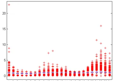
In a preliminary exploratory analysis, the data originally provided consisted in a transformed ratio (in what follows named rescaled data) and revealed serious prob-lems which can be visualized in the boxplot diagrams (Fig. 1). The rescaled data has different distributions and a great number of anomalies per hour. These details are also confirmed in Table 1 where some descriptive statistics and tests are summa-rized.

Fig. 1 Boxplot diagrams (rescaled data 01.01.2008-31.12.2016).

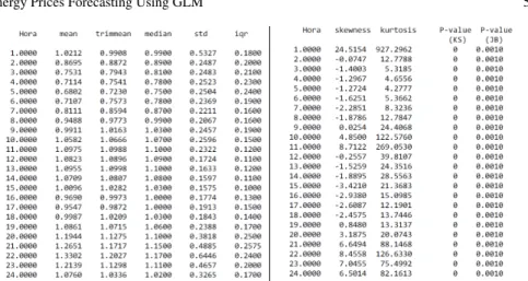
From Table 1, we can see the different patterns of dispersion (observe the stan-dard deviation and inter-quartile range columns respectively). Also we confirm that the data does not have normal distribution when we check the Kolmogorov-Smirnov and Jarcke and Bera normality tests.

Consequently, we consider a new data set with the real data. In a preliminary analysis, we have taken the period from 1st January 2008 to 31st December 2010, to exemplify some details and issues and to estimate the initial models considering several covariates of interest.

Since we have a huge dimensional data set, to compare graphically the rescaled data set and the real data set we restrict to the year 2010 the graphics in Fig. 2. We can conclude that rescaled data present a huge quantity of “uncommon” observa-tions each hour of the day with exception of hours 4, 5 and 6. The rescaled data also presents different patterns of dispersion. By other hand, the real data displays unusual observations but in a fewer quantity than in rescaled data. The dispersion of real data presents more homogeneous patterns each hour.

Table 1 Descriptive summary (rescaled data 01.01.2008-31.12.2016). Left: Mean, trimmean, me-dia, standard deviation, inter-quartile range. Right: Skewness, kurtosis, Kolmogorov-Smirnov, and Jarcke and Bera normality tests.

Fig. 2 Boxplot diagrams of rescaled (left) and real data (right). Time interval: 01.01.2010-31.01.2010.

Considering the real data, for example from January 2008, we found different patterns per day and per hour (see Fig. 3, left).

The same behavior was found in Fig. 3 (right), where, for example, we can see that 22 groups (hours) have mean ranks significantly different from group 1 (hour 1).

Electricity prices can be influenced by the present and past values of various exogenous factors, such as generation capacity, load profiles and meteorological conditions [14], in a preliminary stage we have selected defined and code the fol-lowing candidates to co-variables: Day of the week – C1= 0, 1, 2, 3, 4, 5, 6 (Mon, . . . ,

Sunday); Weekday/Saturday/Sunday – C2= 0, 1, 2; Weekday/Weekend – C3= 0, 1;

Regular day/ holiday – C4= 0, 1; Season – C5= 0, 1, 2, 3 (Winter, Spring, Summer,

Fig. 3 Real data (01.01.2008-31.01.2008). Left: Different patterns per day. Right: Mean price per hour.

3 GLM Approach

In the classical linear model, a vector X with p explanatory variables X = (X1, X2, . . . ,

Xp) can explain the variability of the variable of interest Y (response variable), where

Y = Zβ + ε. Z is a specification matrix with size n × p (usually Z = X , considering an unitary vector in first column), β a parameter vector and ε a vector of random errors εi, independent and identical distributed to a reduced Gaussian.

The data are in the form (yi, xi), i = 1, . . . , n, as result of observation of (Y, X ) n

times. The response variable Y has expected value E[Y |Z] = µ.

GLM is an extension of classical model where the response variable, following an exponential family distribution [13], do not need to be Gaussian. Another extension from the classical model is that the function which relates the expected value and the explanatory variables can be any differentiable function. Yi has expected value

E[Yi|xi] = µi= b0(θi), i = 1, . . . , n.

It is also defined a differentiable and monotone link function g which relates the random component with the systematic component of response variable. The expected value µiis related with the linear predictor ηi= zTiβiusing the relation

µi= h(ηi) = h(zTiβi), ηi= g(µi) (1)

where h is a differentiable function; g = h−1 is the link function; β is a vector of parameter with size p (the same size of the number of explanatory variables); Z is a specification vector with size p.

There are different link functions in GLM. When the random component of re-sponse variable has a Poisson distribution, the link function is logarithmic and the model is log-linear. In particular, when the linear predictor ηi= zTiβicoincides withe

the canonical parameter θi, θi= ηi, which implies θi= zTiβi, the link function is

de-nominated as canonical link function. Sometimes, the link function is unknown, for example, in [7] the link function is estimated simultaneously with the linear compo-nent of the semi-parametric model for electricity spot prices. A detailed description of GLM methodology can be found in several references such as [9], [13].

Initially, to estimate the model as described before, we considered the time inter-val from 01/01/2008 to 31/12/2010. The first approach using IBM SPSS Statistics (version 22) was performed with difficulty due the high dimensionality of data. A question that arose was: ”Can we reduce the number of components of Yt?”, e.g.,

are there significant differences between Yiand Yj, for i 6= j? To solve partially such

issue, we try to reduce the 24 hours of a day to fewer reference hours. First of all, an analysis of data plot per hour was performed. The graphical representation of data (see Fig. 3) shows similar behavior in some distinct. Identified such similar hours we merge them into an unique interval of similarity. In this way the dimension of data can be reduced, by taking the mean or median or other measure of response variable.

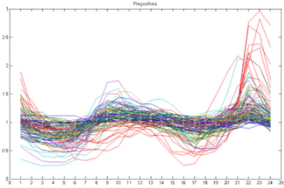
Fig. 4 Data representation (time interval from 01/01/2008 to 31/12/2010).

We have selected and defined some time intervals which conduced to the best model performance. In this way, it was reduced the dimension defining the following time intervals: aurora, lunch time and dinner time. Aurora corresponds to the hours 3, 4 and 5 respectively. Lunch time merges the hours 11, 12, 13 and 14. Dinner time takes into account hours 17, 18 and 19. When the data is graphically overlapped for each hour in the defined time intervals (see Fig. 5) no significant differences were found.

We studied some possible explanatory variables which can contribute to the ex-plication of energy price per hour. In a preliminary stage of the study, using the initial explanatory variables proposed in Sect. 2, an analysis of variance with sec-ond order interaction was performed. The best candidates to explanatory variables of a GLM model were chosen: C1, C4, C5, C6, C7.

It was also considered the fare defined by EDP as possible explanatory variable but it was not significant.

The best models were obtained for log or square root link function. The diagnos-tic analysis and selection of the order of the models was done but we dont reproduce with detail such work. The significant explanatory variables were C4, C6, C7, H2,

Fig. 5 Overlapped data: Aurora time (top), lunch time (center) and dinner time (bottom). Time interval from 01/01/2008 to 31/12/2010.

H7, H8, H16, H20, H22, H23, H24 and lunch time (link fuction: square root). When

we consider the log as link function, the best explanatory variables were C4, C6,

C7, H2, H7, H8, H16, H20, H22, H23, H24. Notice that other transformations should

be considered taking into account the time series nature of the data. Eventually, we could get models with better.

Considering the obtained results as indicators, we can conclude that some of the explanatory variables proposed initially were not relevant for dependent variable, such as, EDP fares, Portuguese holidays (maybe the Iberian holidays can have some relevance, and not just the Portuguese ones). Also, some periods of time can be drop off as relevant explanatory variables, such as dinner time or some others. The season, month or winter/summer time period revealed significant explanatory variables in the different estimated models.

Using this preliminary model estimation as starting point, we repeated all esti-mation process considering a more recent sample so we could compare with the results published in [1]. The GLM model was estimated using hourly prices from 10/03/2014 to 29/5/2016. The remaining sample, from 30/05/2014 to 28/06/2016, was used to evaluate the forecasting performance of the selected model. To asses the in-sample prediction quality of the model, we use the Mean Absolute Percent-age Error (MAPE) and the Root Mean Square Error (RMSE).

Following the preliminary model estimation, in models formulation, we consid-ered the response variable with a Gamma distribution and selected the link function with options: 1-log, 2- square root, 3- identity. We have selected as preliminaries explanatory variables the same used earlier also considered in [1], where its done a VAR approach. There were estimated of model parameters and analyzed the suit-ability measures of estimates. The selection and validation of models such as se-lection of variables, diagnostics, residual analysis and interpretation was concluded. All models obtained good significant results in Likelihood Ratio Chi-Square test, Pearson Chi-Square test, etc. The best models in the sense of performance (estima-tion and forecasting) are the models with the identity link func(estima-tion. The model A (with higher dimensionality), where each hour of the day is considered, has lower performance in sense of residual analysis and forecasting than model B, where we consider the aurora time, lunch time and dinner time and the remaining hours (lower dimensionality).

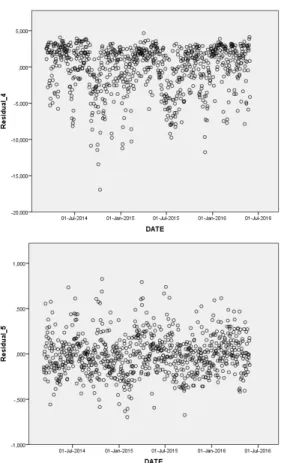
When we analyze the graphics in Fig. 6, we can conclude that model B presents better performance estimation than model A.

From Table 2 we can analyze the quality of prediction in-sample using the MAPE and RMSE. We can conclude that the forecasting quality is promising. In both mod-els (A and B) the prediction performance measures are close, but model B gets better results. Notice that the RMSE values are in accordance with the results obtained us-ing the VAR approach [1].

Fig. 6 Residuals representation (×0.01). Left: Model A. Right: Model B. Estimation period: 10/03/2014 to 29/5/2016.

4 Conclusions and recommendations

The challenge proposed by EDP consisted in simulating electricity prices not only for risk measures purposes but also for scenario analysis in terms of pricing and strategy. Data concerning hourly electricity prices from 2008 to 2016 were provided by EDP.

The data were explored using different statistical software, namely IBM SPSS Statistics, Matlab and R Statistical Software. In this work a GLM approach was considered. The different link functions and the identity case were performed. The season of the year, month or winter/summer period revealed significant explanatory variables in the different estimated models. We got better results when is considered the reduced form of day hours (aurora time, lunch time, dinner time). From Table 2 we can analyze the quality of prediction in-sample by MAPE and RMSE. We can conclude that the forecasting quality is promising. When compared with multivari-ate approach using the VAR approach [1] for the same period (from 30/05/2016 to 28/06/2016) the RMSE values are in accordance with the RMSE computed using the VAR method. Although the forecast do not exactly replicate the real price the results are quite promising. The introduction of other co-variables, such as oil price, gas price, wind energy production, other meteorological variables, would certainly improve the model and the forecast. The GLM approach still needs to be improved in the sense of trying other link functions or some differentiation of data. Others methods should be explored. Longitudinal modeling is an approach which have not yet been addressed in Electricity Price Forecasting and deserves our future attention. Univariate time series is other possible future work.

EPF literature has mainly concerned on models that use information at daily level, however this particularly problem proposed is interested in forecasting intra-day prices using hourly data (disaggregated data), maybe it is necessary to consider models that explore the complex dependence structure of the multivariate price se-ries. The problem of modeling distributional properties of energy prices can be clas-sified in three main classes: reduced form models, forward price models and hybrid price models [5]. Temporal Distribution Extrapolation is another possible idea for our future work.

Acknowledgements This work was supported by Portuguese funds through the Center of Naval Research(CINAV), Portuguese Naval Academy, Portugal and The Portuguese Foundation for Sci-ence and Technology(FCT), through the Center for Computational and Stochastic Mathematics (CEMAT), University of Lisbon, Portugal, project UID/Multi/04621/2013.

References

1. Eliana Costa e Silva, Ana Borges, M. Filomena Teodoro, Marina A. P. Andrade, and Ricardo Covas. Time series data mining for energy prices forecasting: An application to real data. In A. Madureira, A. Abraham, D. Gamboa, and P. Novais, editors, Intelligent Systems Design and

Applications. ISDA 2016., number 557 in Advances in Intelligent Systems and Computing, pages 649–658, New York, 2017. Springer Science+Business Media.

2. S. S. Joens et al. A multivariate time series approach to modeling and forecasting demand in the emergency department. Journal of Biomedical Informatics, 42:123–139, 2009.

3. Y. Fu et al. Arfnns with svr for prediction of chaotic time series with outliers. Expert Systems with Applications, 37:4441–4451, 2014.

4. B. Poczos et. alł. Nonparametric kernel estimators for image classification. Technical report, 2012.

5. A. Eydeland and K. Wolyniec. Energy and power risk management: new developments in modeling, pricing, and hedging. Wiley, New Jersey, 2003.

6. J. W. Taylorł J. M. Jeon. Using conditional kernel density estimation for wind power density forecasting. J. American Statistical Association, 107, 2012.

7. Raimund M. Kocacevic and David Wozabal. A semiparametric model for electricity spot prices. IIE Transactions, 46(4):344–356, 2014.

8. Inna Kolyshkina, Sylvia Wong, and Steven Lim. Enchancing generalised linear models with data mining. Available from http://citeseerx.ist.psu.edu/viewdoc/ summary?doi=10.1.1.566.4377.Lastviewedin08/10/2016.

9. P. McCullagh and J. A. Nelder. Generalized Linear Models. Chapman and Hall, Londres, 1989.

10. G.G.P. Murthy, V. Sedidi, A.K. Panda, and B.N. Rath. Forecasting electricity prices in dereg-ulated wholesale spot electricity market-a review. International Journal of Energy Economics and Policy, 4(1):32, 2014.

11. Saahil Shenoy and Dimitry Gorinevsky. Gaussian-laplacian misture for electricity market. In 2014 IEEE 53rd Annual Conference on Decision and Control (CDC), pages 158–169. IEEE, 2015.

12. L. Su. Prediction of multivariate chaotic time series with local polynomial fitting. Computers & Mathematics with Applications, 59(2):737–744, 2010.

13. M. A. Turkman and G. Silva. Modelos Lineares Generalizados da Teoria ´a Pr´atica. Sociedade Portuguesa de Estast´ıstica, Lisboa, 2000.

14. R. Weron. Electricity price forecasting: A review of the state-of-the-art with a look into the future. International Journal of Forecasting, 30(4):1030–1081, 2014.