ISSN: 1809-4430 (on-line) www.engenhariaagricola.org.br
2 Instituto Nacional de Pesquisas Espaciais/ São José dos Campos - SP, Brasil.
Doi: http://dx.doi.org/10.1590/1809-4430-Eng.Agric.v38n3p387-394/2018
RELATIONSHIP BETWEEN COFFEE CROP PRODUCTIVITY AND VEGETATION
INDEXES DERIVED FROM OLI / LANDSAT-8 SENSOR DATA WITH AND WITHOUT
TOPOGRAPHIC CORRECTION
Sulimar M. C. Nogueira
1*, Maurício A. Moreira
2, Margarete M. L. Volpato
31* Corresponding author. Instituto Nacional de Pesquisas Espaciais/ São José dos Campos - SP, Brasil. E-mail: suli@dsr.inpe.br
KEYWORDS
coffee, NDVI, NDWI,
yield, SAVI, remote
sensing.
ABSTRACT
The reflectance values of a coffee crop are influenced by several factors such as planting
direction, crop spacing, time of the year, plant age and topography which reduces the
accuracy of the estimates derived from remote sensing data.
In this context were evaluated
the relationships between coffee productivity and values of NDVI, SAVI and NDWI
vegetation indexes with and without topographic reflectance correction for different
coffee phenological phases for the crop years 2013/2014 (low productivity) and
2014/2015 (high productivity). The evaluations were made through the standard deviation
of vegetation indices (VIs), linear relationship between the cosine factor and the VIs and
between VIs and coffee productivity.
The best phenological phases of coffee to determine
productivity from spectral indexes were the stages of dormancy and flowering. The results
indicated that the NDVI was the best index to estimate the productivity of coffee trees
with coefficient of determination (R²) that ranged from 0.58 to 0.90.
There was an
increase in R² between productivity and NDVI with topographic correction in the
dormancy phase in the year of low productivity; between productivity and NDVI with
topographic correction in the flowering phase in the year of high productivity; and
between productivity and SAVI and NDWI with topographic corrections in the flowering
phase in the year of high productivity.
INTRODUCTION
Phenological information supports crop productivity and crop management (Sakamoto et al., 2005; Couto Junior et al., 2013). Vegetation indices (VIs) are sensitive to phenological changes and have been used to correlate with agricultural productivity (Bolton & Friedl, 2013; Kogan et al., 2013; Fu et al., 2014), to estimate attributes such as Foliar Area Index that can be related to agricultural yield (Rembold et al., 2013; Taugourdeau et al., 2014;Jiang et al., 2014; Li et al., 2017; Liaqat et al., 2017) or to be incorporated into modeling (Padilla et al., 2012; Meroni et al., 2013; Kowalik et al., 2014). The incorporation of remote sensing data to the modeling improves the estimation of the agricultural yield, since a multispectral evaluation of the cultures state within a certain area can be obtained favoring the study of the relations of the plant with the environment (Delécolle et al., 1992; Rudorff & Batista, 1990).
The spectral behavior of an agricultural crop is related to the way interactions occur between electromagnetic radiation and vegetation characteristics such as vegetation structure, phenological stage, vegetation density, spatial orientation and background soil effects (Galvão et al., 2005; Shimabukuro & Ponzoni, 2012). In areas of perennial crops such as coffee, factors such as soil, systematic use of agricultural implements, internal and inter-row shading, and crop seasonality increase the complexity of the study of coffee spectral characteristics (Epiphanio et al., 1994).
topographic correction on the reflectance values leads to a better prediction of biophysical parameters on vegetation.
As reinforced by Rezende et al. (2014) and Taugourdeau et al. (2014), because it is a complex analysis target, the research on indirect methods of measuring coffee agronomic parameters is scarce. In this context, the objective of this study was to evaluate the relationship between yield of coffee crops and vegetation indexes with and without topographic correction derived from the OLI / Landsat-8 sensor for the 2013/2014 and 2014/2015 crops.
MATERIAL AND METHODS
Study area
This study was carried out in the coffee plantations of Fazenda Conquista from Ipanema Coffees group, located in the municipality of Alfenas in the state of Minas
Gerais, between 21º 14’57”and 21º 20’ 26” South latitude and 45º 54’00” and 45º 59’25” West latitude. The climate of the region is Cwb type with dry winter and mild summer where the average temperature of the hottest month is below 22° C (Alvares et al., 2013).
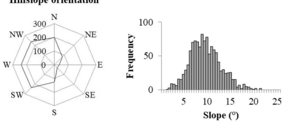
In relation to the slope classes, 64.4% of the study area is located in undulating relief (8 - 20 °), 33.5% in smooth undulating relief (3 - 8 °), 1.8% in flat ground (0 - 3 °) and 0.3% in heavily undulating (20-45 °). Regarding the slope orientation classes, 41.6% of the study area is located in the West facing slopes; 27.9% to the North; 22.7% to the South; and 7.8% to the East. The radial slope orientation frequency profile and slope frequency histogram obtained from the TOPODATA project (Valeriano & Rossetti, 2011), are shown in Figure 1.
FIGURE 1. Radial profile of slope orientation and slope frequency histogram on the study area.
Remote sensing data
Surface reflectance values obtained from OLI / Landsat-8 (Operational Land Imager) images from bands 4 (0.64 - 0.67 μm), 5 (0.85 - 0.88 μm) and 6 (1.57 - 1.65 μm) from orbit / point 219/75 for the crop years 2013/2014 and 2014/2015 years of low and high productivity, respectively.The dates of acquisition of the images used are shown in Table 1. The phenological stages described by Camargo & Camargo (2001) in which the authors divide the coffee cycle of the Arabica species into the Southeast of Brazil into: (I) stage of dormancy of floral buds / beginning of flowering: occurs in the months of July - August - September; (II) flowering stage / beginning of grain formation: occurs between the months of October - November - December; (III) stage of grain formation / beginning of maturation: occurs in the months of January-February-March.
TABLE 1. Dates of OLI / Landsat-8 sensor images used in the study development.
Crop
Phase
I II III
DF –BF (1) F –BGF (2) GF – BM (3)
13/14 Low productivity 07/31/2013 11/20/2013 02/08/2014
14/15 High productivity 03/08/2014 07/11/2014 01/10/2015
(1) Dormancy of floral buds / beginning of flowering; (2) Flowering / beginning of grain formation; (3) Grain formation / beginning of maturation.
Vegetation index
TABLE 2. Summary of vegetation indexes used in this study.
Vegetation Index Equation * Authors
Normalized Difference Vegetation Index
Rouse et al. (1973)
Soil-Adjusted Vegetation Index
Huete (1988)
Normalized Difference Water Index
Gao (1996) * = near infrared reflectance; = reflectance in red; = shortwave infrared reflectance; and constant L = 1.
Correction of surface reflectance according to soil topography
In flat soil the influence of the topography on the reflectance is zero. However, in areas in which topography presents variations in slope and slope orientations, the influence of the topographic effect on the spectral data can be significant (Moreira, 2014). The effect of topography can be minimized by taking into account the angle of solar incidence on the surface of the terrain (cosine factor), determined from the azimuthal and solar zenith angles, the slope (zenith angle from normal to the surface) and the hillslopes orientation (azimuthal angle on the normal surface). The calculation of the cosine factor (cos i), according to Sellers (1965) can be obtained according to [eq. (1)]:
(1) On that,
= solar zenith angle, [degree];
= slope, [degree];
= solar azimuth angle, [degree]; and
= hillslope orientation, [degree].
The cos i can present values between 0 and 1. Values near 0 correspond to dimly lit areas ( ~ 90° and elevation angle ~ 0°) and values close to 1 correspond to the illuminated areas ( ~ 0° and elevation angle ~ 90°) (Lima & Ribeiro, 2014). According to the results found by Moreira & Valeriano (2014) it was tested for this study the SCS + C method of Soenen et al. (2005) (Equations. 2 to 4).
(2)
On that: (3) And,
(4) On that,
= corrected band reflectance λ; = original band reflectance λ;
= coefficient of the line, and
= constant determined individually for each studied field.
The non-Lambertian correction method presented in [eq. (2)] considers the effects of the irradiance variation in each spectral band through constants obtained by the regression method between the reflectance and the angle of solar incidence on the surface. The SCS + C method is based on the C correction of Teillet et al. (1982) with addition of the Sun-Canopy-Sensor method (SCS). By including the slope of the terrestrial surface, the SCS + C method considers the influence of the diffuse irradiance on the canopy spectral response. In the Teillet et al. (1982) method, the constant Cλ is used to model diffuse irradiance
and exerts a moderating influence on cosine correction increasing the denominator and reducing overcorrection of dimly lit pixels (Soenen et al., 2005).
We used the solar angles (θs and φs) available in the metadata image and the soil angles (θt and φt) that were determined from the digital elevation model (DEM) from the TOPODATA project. After the determination of the cosine factor, the reflectance was corrected for each pixel and spectral band of the image. Since the coffee areas show variations in planting, spacing and plant age, the determination of the cosine factor and the topographic correction were done individually by the coffee field, so that the crop variations on the reflectance values were taken in consideration.
Determination of average values on vegetation index
From the thematic map with the spatial distribution of the coffee plantations given by the technicians from the Conquista farm, it was generated a mask of the coffee plantations with pixels size of 30 m, compatible with the images from the Landsat satellite. On this mask were selected areas with 100% of coffee occupation to obtain reflectance values, thus excluding edge pixels with presence of other targets.
The reflectance values were used to determine the NDVI, SAVI and NDWI index and their corresponding values corrected by topography (NDVIcorr, SAVIcorr and
NDWIcorr). Subsequently, we obtained the average values
of this vegetation index per plot.
Relationship between coffee productivity and VIs with and without topographical correction
determinate the relationship between productivity data (t ha-1) and the mean values of VIs with and without
topographic correction per plot. The analysis was conducted by the simple regression method obtaining the coefficient of determination (R²) which was submitted to the analysis of significance by means of the p-value of the F-test for regression analysis at a significance level of 5%.
The quantitative analysis of the validity of the correction method used in the study was made by determining the standard deviation of the data with and without topographic correction, once the topographic effect was removed, the corrected image variance was lower (Hantson & Chuvieco, 2011), besides the calculation of the coefficient of determination between the reflectance values (with and without topographic correction) and the cosine factor, since this relation decreases after the topographic correction (Lima & Ribeiro, 2014).
RESULTS AND DISCUSSION
Analysis of the relationship between VIs with and without correction of topographic effect
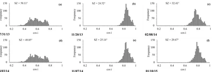
Figure 2 shows the frequency histograms on mean values of cos i and zenith angles for the considered period in this study. The mean cosine factor varied between 0.49 and 0.94 with a minimum of 0.33 and a maximum of 0.97. Low values of cos i indicate that some areas receive poor lighting while areas of cos i close to 1 indicate well-lit ones. There were no values of cosine factor lower than or equal to zero, so all analyzed plots received direct solar illumination at the moment of the satellite crossing in accordance with the results by Moreira (2014). High mean values of cos i observed in periods of low solar zenith (SZ) (lower than 30 °), indicate well-lit areas and little shade as stated by Lima & Ribeiro (2014).
FIGURE 2. Histogram of frequency values of cos i medium and zenith angle (°) in the study area for the images obtained in the year of low productivity: (a) July 31, 2013, (b) November 20, 2013, (c) February 8, 2014; and in the year of high productivity: (d) August 3, 2014, (e) July 7, 2014 and (f) January 10, 2015. (SZ = solar Zenith).
From the analysis on the values of determination coefficient (R2) (Figure 3) it is verified that, in general, the
NDWI index presented higher values of R2 with the cosine
factor, except for the dates of July 31, 2013 and November 20, 2013 in which the sensitivity of NDVI and SAVI index in relation to the topography varied between plots. On July 31, 2013 SAVI presented the highest values of R2 for plots
1, 4, 5 and 8, while NDVI showed higher correlations with cosine factor for plots 2, 3 and 7. On November 20, 2013 SAVI was more sensitive to topography, that is, higher
correlation with cos i, except for plot 5 and 8. However, in the year of high productivity (2014/2015), SAVI presented lower correlation with cosine factor, with NDVI being more sensitive to topographic effects.
In relation to the topographic correction (Figure 3) there was decreasing in R2 values among the vegetation
index and cosine factor (R2 values close and / or equal
FIGURE 3. Coefficient of determination (R²) between the cosine factor and the uncorrected VIs, and Coefficient of determination (R² CORRECTED) between the cosine factor and VIs with correction by the SCS + C method for obtained images in the year of low productivity: (a) July 31, 2013, (b) November 20,2013 and (c) February 8, 2014; and for the images obtained in the high productivity year: (d) August 3, 2014, (e) November 7, 2014 and (f) January 10,2015.
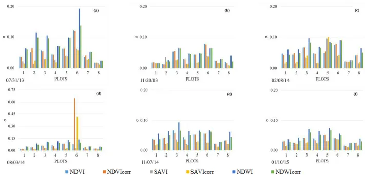
Figure 4 shows the standard deviations of vegetation indices before and after the topographical corrections on spectral bands. In general, there was a reduction in the standard deviation values of the NDWI. It was not observed on corrected image, values of standard deviation higher than the original image. For NDVI and SAVI the values of standard deviation of some corrected data were higher than those obtained from the original images indicating inefficiency of the method by Soenen et al. (2005) to remove the variance from the original image. Similar results were reported by Hantson & Chuvieco (2011) and Moreira & Valeriano (2014) in the study of individual bands.
FIGURE 4. Standard deviation of the VIs without corrections (NDVI, SAVI and NDWI) and VIs corrected (NDVIcorr, SAVIcorr and
NDWIcorr) by the SCS + C method for obtained images in the year of low productivity: (a) July 31, 2013, (b) November 20, 2013, (c)
Analysis of the relationship between VIs and coffee productivity
Table 3 shows the values of determination coefficients between three vegetation indexes with and without topographic correction and coffee productivity.
TABLE 3. Determination coefficient (R2) and p-value between vegetation indexes with and without topographic correction by the SCS + C method and coffee productivity in 2013/14 and 2014/15 crops.
Crop Date Phase(1) NDVIMEDIUM NDVIMEDIUM - Corrected
R2 p-Value R2 p-Value
L
ow 07/31/13 11/20/13 II I 0.62 0.58 0.02 0.03 0.71 0.51 0.01 0.05
02/08/14 III 0.46n.s. 0.06 0.25n.s. 0.21
Hig
h 08/03/14 I 0.89 0.00 0.57 0.03
11/07/14 II 0.73 0.01 0.81 0.00
01/10/15 III 0.22n.s. 0.24 0.28n.s. 0.17
Crop Date Phase SAVIMEDIUM SAVIMEDIUM - Corrected
R2 p-Value R2 p-Value
L
ow 07/31/13 I 0.60 0.02 0.47
n.s. 0.06
11/20/13 II 0.44n.s. 0.07 0.37n.s. 0.11
02/08/14 III 0.55 0.03 0.43n.s. 0.07
Hig
h 08/03/14 I 0.85 0.00 0.78 0.00
07/11/14 II 0.88 0.00 0,89 0.00
01/10/15 III 0.10n.s. 0.44 0.16n.s. 0.33
Crop Date Phase NDWIMEDIUM NDWIMEDIUM - Corrected
R2 p-Value R2 p-Value
L
ow 07/31/13 11/20/13 II I 0.460.70 n.s. 0.01 0.06 0.350.65 n.s. 0.01 0.12
02/08/14 III 0.48n.s. 0.06 0.32n.s. 0.14
Hig
h 08/03/14 I 0.89 0.00 0.78 0.00
11/07/14 II 0.64 0.02 0.81 0.00
01/10/15 III 0.16n.s. 0.33 0.23n.s. 0,23
(1) I: Dormancy of floral buds / beginning of flowering; II: Flowering / beginning of grains formation; III: Grains formation / beginning of maturation.
P-value for the F test of the regression analysis for significance of 5%; n.s.(not significant)
The data in Table 3 show that agricultural productivity is correlated with the NDVI values in phases I and II, for both low and high production years. In the low production year (2013/14) the determination coefficient values were 0.62; 058; 0.46 (not significant) for phase I, II and III. In the year of high production (2014/15) the determination coefficient was 0.89; 0.73; 0.22 (not significant), for phases I, II and III, respectively, which explained the coffee productivity in 89%, 73% and 22% respectively. The determination coefficient values decreased from phase I to III. The results corroborate with values found by Bernardes et al. (2012) who found higher correlation between coffee productivity and NDVI in the period of August / September. This fact may be associated to an increase in leaf area index that cause an increase in internal shading and, consequently, a change in crop reflectance.
The determination coefficient of NDVI values after topographic correction increased from 0.62 to 0.71 in phase I in the year of low productivity and from 0.73 to 0.81 in phase II in the year of high productivity.
In general, the SAVI index presented a lower relation with productivity data when compared to the other index. As discussed for the NDVI, in the year of low production the determination coefficient values were lower compared to the year of high coffee production. The determination coefficient between SAVI and productivity was 0.60 and 0.85 in phase I in the crop years 2013/2014
and 2014/2015 respectively. In phase II, the R² was 0.44 (not significant) in the year of low productivity and of 0.88 in the year of high productivity. In the period of grain formation and maturation (phase III), the SAVI presented determination coefficient of 0.55 in the year of low productivity and 0.10 (not significant) in the year of high productivity.
The NDWI presented higher correlation with the productivity data in the dormancy period (phase I) for the two-year crop with determination coefficient (R2) of 0.70
and 0.89 for the crop years 2013/2014 and 2014/2015 , respectively. In addition to the relationship with lower canopy internal shading (Epiphanio et al., 1994), coffee cultivation is highly dependent on water availability which is the main factor affecting productivity (Picini et al., 1999). Thus, index that use spectral information of the medium infrared (energy absorbed by water) may present better results. After the topographic correction was verified correlation with productivity only for phases II and III in the year of high productivity with determination coefficient increasing from 0.64 to 0.81 in phase II and from 0.16 (not significant ) to 0.23 (not significant) in phase III.
CONCLUSIONS
from the Landsat-8 / OLI satellite for 2013/2014 and 2014/2015 crops, and according to the results of the research it can be conclude that the SAVI index presented a lower relation with the productivity data when compared to the other two index. In addition, the three indexes showed higher values of determination coefficients in the years of high productivity, coinciding with the lower index of leaf area, besides greater contribution on the bottom surface.
The analyses of the correlation of the three vegetation indexes with the productivity for coffee trees conclude that the best correlations among the VIs and productivity were obtained for the stages of dormancy and flowering. Among the analyzed indexes the NDWI presented higher determination coefficient (R2) at the
dormancy stage for two analyzed years (R2 between 0.69
and 0.89).
In two years of study the NDVI obtained the best correlations with productivity in the dormancy and flowering stages. This index explained the productivity variation between 62% and 89% of the data observed in the dormancy stage and from 58% to 73% in the flowering stage.
The topographic correction method reduced the correlation between vegetation index and cosine factor to zero in most of the analyzed dates. However, inefficiency of the method was observed in decreasing the standard deviation of NDVI and SAVI data.
Topographic correction increased the determination coefficient between productivity and the three indexes in phase II in the year of high productivity and in phase I in the year of low productivity for the NDVI index.
It is emphasized that additional studies are needed to evaluate the efficiency of other methods of topographical correction in coffee areas and its implication on the correlation between vegetation indexes and agricultural productivity.
REFERENCES
Alvares CA, Stape JL, Sentelhas PC, Gonçalves JLM, Sparovek G (2013) Köppen’s climate classification map for Brazil. Meteorologische Zeitschrift 22(6):711–728. Bernardes T, Moreira MA, Adami M, Giarolla A, Rudorff BFT (2012) Monitoring biennial bearing effect on coffee yield using MODIS remote sensing imagery. Remote Sensing 4:2492-2509.
Bolton DK, Friedl MA (2013) Forecasting crop yield using remotely sensed vegetation indices and crop phenology metrics. Agricultural and Forest Meteorology 173:74-84. Camargo AP, Camargo MBP (2001) Definição e
esquematização das fases fenológicas do cafeeiro arábica nas condições tropicais do Brasil. Bragantia 60 (1):65-68. DOI:
http://dx.doi.org/10.1590/S0006-87052001000100008
Couto Junior AF, Carvalho Junior OA, Martins ES, Guerra AF (2013) Phenological characterization of coffee crop (Coffea arabica L.) from Modis time series. Revista
Delécolle R, Maas SJ, Guérif M, Baret F (1992) Remote sensing and crop production models: present trends. ISPRS Journal of Photogrammetry and Remote Sensing 47:145-161.
Ediriweera S, Pathirana S, Danaher T, Nichols D, Moffiet T (2013) Evaluation of different topographic corrections for Landsat TM data by prediction of Foliage Projective Cover (FPC) in topographically complex landscapes. Remote Sensing 5:6767-6789.
Epiphanio JCN, Leonardi L, Formaggio AR (1994) Relações entre parâmetros culturais e resposta espectral de cafezais. Pesquisa Agropecuária Brasileira 29 (3):439-447. Fu Y, Yang G, Wang J, Song X, Feng H (2014) Winter wheat biomass estimation based on spectral indices, band depth, analysis and partial least squares regression using hyperespectral measurements. Computers and Electronics in Agriculture 100:51-59.
Galvão LS, Formaggio AR, Tisot DA (2005)
Discrimination of sugarcane varieties in Southeastern Brazil with EO-1 Hyperion data. Remote Sensing of Environment 94:523-534.
Gao B (1996) NDWI - A Normalized Difference Water Index for remote sensing of vegetation liquid water from space. Remote Sensing of Environment 58:257-266. Hantson S, Chuvieco E (2011) Evaluation of different topographic correction methods for Landsat imagery. International Journal of Applied Earth Observation and Geoinformation13:691-700.
Huete AR (1988) A Soil-Adjusted Vegetation Index (SAVI). Remote Sensing of Environment 25:295-309. Jiang ZW, Chen ZX, Chen J, Liu J, Ren JQ, Li ZN, Sun L, LI H (2014) Application of crop model data assimilation with a particle filter for estimating regional winter wheat yields. IEEE Journal of Selected Topics in Applied Earth Observations and Remote Sensing 7:4422-4431.
Kogan F, Kussul N, Adamenko T, Skakun S, Kravchenko O, Kryvobok O, Shelestov A, Kolotii A, Kussul O, Lavrenyuk A (2013) Winter wheat yield forecasting in Ukraine based on Earth observation, meteorological data and biophysical models. International Journal of Applied Earth Observation and Geoinformation 23:192-203. Kowalik W, Dabrowska-Zielinska K, Meroni M, Raczka TU, de Wit A (2014) Yield estimation using SPOT-VEGETATION products: A case study of wheat in European countries. International Journal of Applied Earth Observation and Geoinformation 32:228-239.
Li H, Chen Z, Jiang Z, Wu W, Ren J, Liu B (2017) Comparative analysis of GF-1, HJ-1, and Landsat-8 data for estimating the leaf area index of winter wheat. Journal of Integrative Agriculture 16(2):266-285.
Lima RNS, Ribeiro CB (2014) Comparação de métodos de correção topográfica em imagens Landsat sob diferentes condições de iluminação. Revista Brasileira de Cartografia 66(5):1097-1116.
Mattar C, Franch B, Sobrino JA, Corbari C, Jiménez-Muñoz JC, Olivera-Guerra L, Skokovic D, Sória G, Oltra-Carriò R, Julien Y, Mancini M (2014) Impacts of the broadband albedo on actual evapotranspiration estimated by S-SEBI model over an agricultural area. Remote Sensing of Environment 147:23-43.
Meroni M, Marinho E, Sghaier N, Verstrate MM, Leo O (2013) Remote Sensing Based Yield Estimation in a Stochastic Framework — Case Study of Durum Wheat in Tunisia. Remote Sensing 5:539-557.
Moreira EP (2014) Correção radiométrica do efeito de iluminação solar induzido pela topografia. Dissertação Mestrado, Instituto Nacional de Pesquisas Espaciais, Sensoriamento Remoto.
Moreira EP, Valeriano MM (2014) Application and evaluation of topographic correction methods to improve land cover mapping using object-based classification. International Journal of Applied Earth Observation and Geoinformation 32:208-217.
Moreira EP, Valeriano MM, Sanches IDA, Formaggio AR (2016) Topographic effect on spectral vegetation indices from Landsat TM data: is topographic correction
necessary? Boletim de Ciências Geodésicas 22(1):95-107. Padilla FLM, Maas SJ, González-Dugo MP, Mansilla F, Rajan N, Gavilána P, Domínguez J (2012) Monitoring regional wheat yield in Southern Spain using the GRAMI model and satellite imagery. Field Crops Research 130:145-154.
Picini AG, Camargo MBP, Ortolani AA, Fazuoli LC, Gallo PB (1999) Desenvolvimento e teste de modelos agrometeorológicos para a estimativa de produtividade do cafeeiro. Bragantia 58:157-170.
Shimabukuro YE, Ponzoni FJ (2012) Orbital sensors data applied to vegetation studies. Revista Brasileira de Cartografia 6:873-886.
Rembold F, Atzberger C, Savin I, Rojas O (2013) Using Low Resolution Satellite Imagery for Yield Prediction and Yield Anomaly Detection. Remote Sensing 5:1704-1733. Rezende FC, Caldas ALD, Scalco MS, Faria MA (2014) Índice de área foliar, densidade de plantio e manejo de irrigação do cafeeiro. Coffee Science 9:374-384. Rouse JW, Haas RH, Schell JA, Deering DW (1973) Monitoring vegetation systems in the Great Plains with ERTS. In: Earth Resources Technology Satellite-1 Symposium. Washington, NASA, Proceedings… Rudorff BFT, Batista GT (1990) Yield Estimation of Sugarcane Based on Agrometeorological- Spectral Models. Remote Sensing of Environment 33:183-192.
Sakamoto T, Yokozawa M, Toritani H, Shibayama M, Ishitsuka N, Ohno H (2005) A crop phenology detection method using time-series MODIS data. Remote Sensing of Environment 96:366-374.
Sellers WD (1965) Physical climatology. Chicago, University of Chicago Press, 272p.
Soenen SA, Peddle DR, Coburn CA (2005) SCS+C: a modified sun-canopy sensor topographic correction in forested terrain. IEEE Transactions on Geoscience and Remote Sensing 43(9):2148-2159.
Taugourdeau S, Maire G, Avelino J, Jones JR, Ramirez LG, Quesada MJ, Charbonnier F, Gómez-Delgado F, Harmand J, Rapidel B, Vaast P, Roupsard O (2014) Leaf area index as an indicator of ecosystem services and management practices: An application for coffee agroforestry. Agriculture, Ecosystems and Environment 192:19-37.
Teillet PM, Guindon B, Goodenough DG (1982) On the slope-aspect correction of multispectral scanner data. Canadian Journal of Remote Sensing 8:84-106.