Analytical Model for the Performance Curves of a Family of Propellers based on Wind Tunnel Tests

(1)

UNIVERSIDADE DA BEIRA INTERIOR

Engenharia

Analytical Model for the Performance Curves of a

Family of Propellers based on Wind Tunnel Tests

(versão corrigida após defesa)

Miguel Cabeleira dos Santos

Dissertação para obtenção do Grau de Mestre em

Engenharia Aeronáutica

(Ciclo de Estudos Integrado)

Orientador: Prof. Doutor Pedro Vieira Gamboa

(2)

(3)

Acknowledgments

First and foremost, I would like to acknowledge my supervisor, Professor Pedro Vieira Gamboa, for all the patience and guidance throughout the duration of this work.

I want to acknowledge Engineer Pedro Alves for the help provided while mounting the experimental setup in the wind tunnel at University of Beira Interior, guiding me through the wind tunnel tests and sharing his knowledge and experience with me.

I would like to thank all my friends at Desertuna for all the help and support they gave me during this chapter of my life, thanks to them, I learned numerous things and surpassed many challenges.

I want to thank all my true friends, I will never forget them, for their support and friendship. A special thank you to Alexandre Nunes, Beatriz Leal, Inês Cruz, Luís Correia and Mariana Costa. Above all, I would like to thank my parents, João and Lídia, and my sister, Joana, for all the motivation and support given to me through my whole life.

(4)

(5)

Resumo

O principal objetivo do trabalho levado a cabo nesta dissertação é a construção e validação de um modelo analítico para o desempenho de uma família de hélices com base em dados experimentais em condições de baixo número de Reynolds. Este tipo de hélices é mais utilizado em Veículos Aéreos Não Tripulados (VANTs).

O modelo foi projetado em MATLAB® utilizando vários métodos de regressão, tal como o método dos mínimos quadrados (MMQ), baseado em dados experimentais obtidos na Universidade de Illinois em Urbana-Champaign (UIUC), de dezassete hélices testadas da APC Thin Electric. Os dados experimentais passaram por um processo de redução para um tratamento de dados mais facilitado. No âmbito do desenvolvimento deste modelo, foram feitos testes no Departamento de Ciências Aerospaciais (DCA), na Universidade da Beira Interior (UBI) a mais dez hélices da APC Thin Electric.

O modelo analítico permite calcular os valores para o coeficiente de potência e para a eficiência propulsiva para hélices com dimensões próximas ou iguais das que foram utilizadas para a sua construção. Este modelo será útil para proporcionar uma melhor fase de projeto, providenciando uma mais rápida e eficiente seleção de hélice. Os dados dos testes ao desempenho das hélices obtidos durante o processo experimental foram catalogados para aumentar a documentação existente sobre hélices testadas em condições de baixo número de Reynolds.

Palavras-chave

(6)

(7)

Abstract

The main objective of the work done in this dissertation is the construction and validation of an analytical model for the performance curves of a family of propellers tested at low Reynolds numbers. This kind of propellers is more commonly used in Unmanned Aerial Vehicles (UAVs). The model was designed in MATLAB® using a variety of regression techniques, such as the Least Squares Method (LSQ), via experimental data acquired at University of Illinois at Urbana-Champaign (UIUC), of measurements of seventeen APC Thin Electric propellers. The experimental data went through a reduction process for easier analysis. In order to further develop this model, tests were run at the Department of Aerospace Sciences (DCA) of University of Beira Interior (UBI) for ten more APC Thin Electric propellers.

The analytical model will predict power coefficient and propeller efficiency accurately for the propellers with dimensions close to those that were used for its development. This model will be useful to achieve optimal design, providing a faster and more efficient propeller selection phase. The propeller performance obtained during the experimental tests will also be catalogued to further increase the documentation on propellers tested at LRN.

Keywords

(8)

(9)

List of Figures

Figure 1 - Typical representation of propeller efficiency curves (McCormick, 1979). ... 4

Figure 2 - Typical representation of propeller thrust coefficient curves (McCormick, 1979). ... 4

Figure 3 - Typical representation of propeller power coefficient curves (McCormick, 1979). ... 5

Figure 4 - Schematic of the Wind Tunnel at UBI. ... 8

Figure 5 - Divided Difference table [19]. ... 10

Figure 6 - Experimental Setup designed by Alves [16]. ... 11

Figure 7 - Data acquisition program interface. ... 13

Figure 8 - Example of data points of 𝐶𝑃 and 𝐶𝑃𝑟. ... 15

Figure 9 - Example of data points of 𝜂 and 𝜂𝑟. ... 16

Figure 10 - Dispersion for propellers with 𝑝 𝐷 ratio of 0.5 (a and b) and the results of lsqlin function in MATLAB® (c). ... 22

Figure 11 - 1 of 2 different behaviors of data for propellers with 𝑝 𝐷 ratio not equal to 0.5 (a, b, c, and d) and the results of lsqlin function in MATLAB® (e). ... 23

Figure 12 - 2 of 2 different behaviors of data for propeller with 𝑝 𝐷 not equal to 0.5 (a, b, c) and the results of lsqlin function in MATLAB® (d). ... 24

Figure 13 - 3D plot of 𝐶𝑃1. ... 27

Figure 14 - 3D plot of 𝐶P2,3. ... 30

Figure 15 - 1 of 2 behaviors of propeller efficiency when 𝑝 𝐷> 0.9 ... 31

Figure 16 - 2 of 2 behaviors of propeller efficiency when 𝑝 𝐷< 0.9. ... 31

Figure 17 - 3D plot of 𝜂1. ... 33

Figure 18 - 𝐽𝑚𝑎𝑥(𝐷, 𝑝). ... 34

Figure 19 - 𝐶𝑃𝑟0(𝐷, 𝑝). ... 35

Figure 20 - 𝜂𝑟𝑚𝑎𝑥(𝐷, 𝑝) ... 36

Figure 21 - Propeller Performance comparison with UIUC data for propeller 8x4. ... 39

Figure 24 - Propeller Performance comparison with UIUC data for propeller 9x4.5. ... 40

(12)

Figure 32 - Propeller Performance comparison with UIUC data for propeller 11x8... 42

Figure 38 - Testing of the first model with data from propeller 7x4. ... 45

Figure 48 - Representation of the propellers used to create (data acquired from UIUC, circles) and validate (data acquired at UBI, triangles) the analytical model. ... 49

Figure 49 - Dispersion for propellers with 𝑝 𝐷 ratio lower than 0.6 (a, b and c) and the results of lsqlin function in MATLAB® (d). ... 50

Figure 50 - Dispersion for propellers with 𝑝 𝐷 ratio between 0.6 and 0.8 (a, b, c and d) and the results of lsqlin function in MATLAB® (e). ... 51

Figure 51 - Dispersion for propellers with 𝑝 𝐷 ratio higher than 0.8 (a, b) and the results of lsqlin function in MATLAB® (c). ... 52 Figure 52 - 3D plot of 𝐶𝑃𝑟 𝐶𝑃𝑟0( 𝐽 𝐽𝑚𝑎𝑥, 𝑝 𝐷). ... 54

Figure 53 - 1 of 3 behaviors of propeller efficiency for 𝑝 𝐷> 0.9 ... 55

Figure 54 - 2 of 3 behaviors of propeller efficiency for 0.5 <𝑝 𝐷< 0.9 ... 55

Figure 55 - 3 of 3 behaviors of propeller efficiency for 𝑝 𝐷< 0.5. ... 56 Figure 56 - 3D plot of 𝜂𝑟 𝜂𝑟𝑚𝑎𝑥( 𝐽 𝐽𝑚𝑎𝑥, 𝑝 𝐷). ... 57 Figure 57 - 3D plot of 𝐽𝑚𝑎𝑥(𝐷, 𝑝). ... 59 Figure 58 - 3D plot of 𝐶𝑃𝑟0(𝐷, 𝑝)... 60 Figure 59 - 3D plot of 𝜂𝑟𝑚𝑎𝑥(𝐷, 𝑝) ... 61

Figure 60 - Propeller Performance comparison with UBI data for propeller 7x4. ... 63

(13)

(14)

(15)

List of Tables

Table 1 - Convergence criteria to achieve wind tunnel freestream speed and propeller’s RPM steady. ... 12 Table 2 - Values of D, p, 𝐶𝑃𝑟0 and

𝐷+𝑝

CPr0 for each propeller with

𝑝

𝐷≠ 0.5 : ... 25

Table 3 - Values of D, p and 𝐶𝑃𝑟0 for propeller with 𝑝

𝐷= 0.5. ... 25

Table 4 - Averages of propellers' 𝑝

𝐷 ratio. ... 32

Table 5 - Values of 𝐷, 𝑝, 𝐽𝑚𝑎𝑥, 𝐶𝑃𝑟0 and 𝜂𝑟𝑚𝑎𝑥 used in the plotting of the functions above. .. 37

Table 6 - Mean relative error of the model's predictions for the first model. ... 38 Table 7 - Mean relative error (MRE), 𝛿𝑚𝑎𝑥 and standard deviation of the model's prediction of the propeller's tested at UBI. ... 45 Table 8 - Values of 𝐷, 𝑝, 𝐽𝑚𝑎𝑥 , 𝐶𝑃𝑟0 and 𝜂𝑟𝑚𝑎𝑥 for each propeller. ... 58

Table 9 - Mean relative error, Max relative error and standard deviation of the model’s prediction of all the propellers and total 𝑅2_{value. ... 62}

(16)

(17)

Lista de Acrónimos

APC Advanced Precision Composites BEM Blade Element Momentum Theory DCA Department of Aerospace Sciences GPL General Public License

LRN Low Reynolds Number LSQ Linear Least Squares Method MATLAB Matrix Laboratory

MIT Massachusetts Institute of Technology MRE Mean Relative Error

NACA National Advisory Committee for Aeronautics RSM Response Surface Models

UBI Universidade da Beira Interior

(18)

(19)

Nomenclature

c Propeller blade chord, m.

𝐶𝑃 Power Coefficient.

𝐶𝑄 Torque Coefficient.

𝐶𝑇 Thrust coefficient.

D Propeller diameter, in.

J Advance Ratio.

n Rotational speed, cycles/s.

N Rotational speed, cycles/min.

p Propeller pitch, in.

P Power, W.

Patm Atmospheric pressure, Pa.

Q Torque, Nm.

R Air constant, 𝑅 = 287 J·kg-1_·K-1_.

R2 _{Coefficient of determination.}

Re Reynolds number.

T Thrust, N.

Tatm Atmospheric temperature, K.

V Freestream velocity, m/s.

Greek parameters

𝛿 Relative error, %

𝛿𝑚𝑎𝑥 Maximum relative error, %

η Propeller efficiency. μ Dynamic viscosity, kg/ms.

(20)

(21)

Chapter 1

Introduction

In the introductive chapter to this study, the motivation to develop the analytical model is explained, the objectives of the study are enumerated, and a section explaining the structure of this document is presented.

1.1 Motivation

With the Unmanned Aerial Vehicle industry becoming larger in modern times, the design of UAVs becomes more important every day. An efficient airplane requires a rigorous design, and this includes its propulsive systems. Most UAVs propulsive systems use propellers to generate the thrust they need to fly, which can be evaluated by measuring the thrust and power coefficients and propeller efficiency. Good predictions of these performance curves will be a great asset during preliminary design, or UAV optimization problems.

A study conducted by Brandt and Selig [1] shows that propeller efficiencies vary greatly depending on the propeller, thus, making an accurate prediction of propeller performance curves, can greatly improve overall UAV design productivity and optimization procedures. This selection requires many tests in wind tunnels to acquire enough data to analyze the propeller’s performance. To conduct tests for propellers in a wind tunnel, the latter must be equipped with an experimental setup designed to place a propeller inside the test section, and each test takes around two hours, depending on the number of different propeller speeds one desires to test, and the number of freestream velocity points to analyze. Therewith the construction of an analytical model will enable to rapidly develop and test different propeller designs, compare them, make small changes and test again, without the complexity of wind tunnel tests, and in the end, when a reduced sample of propellers has been attained, one can study them in greater detail at a wind tunnel.

(22)

1.2 Objectives

The goal of this work is to design a mathematical model for propeller performance of a family of propellers, namely the Thin Electric Propellers of the brand APC. To achieve this, the work is divided in two phases:

• The first is to construct the model using data provided by UIUC;

• The second phase includes tests conducted at UBI in order to collect experimental propeller performance data to further develop the analytical model.

The second phase is also important, because of the lack of documentation on propellers studied at LRN conditions, for the characterization of uncatalogued propellers performance.

1.3 Document Structure

The document starts with a brief introduction explaining the motivation and the objectives of this work. Following, is the state of the art, where the propeller’s characteristics are explained, the most relevant parameters for propeller performance analysis and an example of the curve behavior of such parameters. Thereafter, some examples of already existing programs that analyze the propeller’s performance are displayed followed by a brief explanation on how important surrogate models based on experimental data are. This chapter will be finished with a small section that presents some of the experimental studies over the propellers tested at Low Reynolds Numbers (LRN). The third chapter includes the experimental procedure for testing these propellers at the wind tunnel at UBI, followed by the data reduction procedure, also an explanation about the most common and effective regression techniques and validation of curve fits is provided. In the fourth chapter, the results of this study are shown, the first model presented was created with the data retrieved from UIUC Propeller Database [2], and then it was used the same model to predict the propeller’s performance tests at UBI, comparing the results. Finally, the updated analytical model with both data retrieved from UIUC [2] and data collected from tests conducted at UBI will be presented along with the statistical validation with error calculation and the coefficient of determination for both 𝐶𝑃 and 𝜂. Finally,

the fifth chapter will provide a conclusion about this project and some of the work that can be conducted in the future.

(23)

Chapter 2

State of the Art

In this chapter a brief explanation on which propeller’s characteristics are relevant to this study is shown, followed by a list of already existing propeller performance parameter programs available online. In the end of this section, a brief sample of experimental studies conducted prior to this research are displayed.

2.1 Propeller’s Characteristics

A propeller uses its blade’s rotation, which acts as a rotating wing, to produce lift and drag. Propeller nomenclature is usually a set of two numbers. The first one is the total propeller diameter, and the second is the pitch of the propeller blades themselves, which refers to the angle between the propeller blade chord line and the plane of rotation of the propeller. Blade pitch is most often described in terms of units of distance that the propeller would move forward in one rotation. For instance, when naming a 10x5 propeller, it means that it has a 10-inch diameter and a 5-10-inch blade pitch.

The propeller’s performance is evaluated by the thrust and power coefficients, 𝐶𝑇 and 𝐶𝑃,

respectively, which depend primarily on the advance ratio, J, the blade Reynolds number Re, and on the propeller geometry [3].

𝐶𝑇= 𝐶𝑇(𝐽, 𝑅𝑒, 𝑔𝑒𝑜𝑚𝑒𝑡𝑟𝑦) (2.1) 𝐶𝑃= 𝐶𝑃(𝐽, 𝑅𝑒, 𝑔𝑒𝑜𝑚𝑒𝑡𝑟𝑦) (2.2) 𝐽 = 𝑉 𝑛𝐷 (2.3) 𝑅𝑒 =𝜌𝑉𝑐 𝜇 (2.4)

where 𝑉 is the freestream velocity, n is the propeller’s rotational speed, in cycle/s, D is diameter, Re is the Reynolds number, ρ is the air density, c is propeller blade chord and 𝜇 is the dynamic viscosity of the fluid.

(24)

Once the propeller geometry is known, and the coefficients and propeller efficiency, 𝜂, have been generated by measurement or analysis, the thrust, T, and torque, Q, can be calculated for any other V and n by dimensionalizing the coefficients:

𝜂 =𝐶𝑇𝐽 𝐶𝑃 (2.5) 𝑇(𝑛, 𝑉) =1 2𝜌(𝑛𝐷) 2_{𝜋 (}𝐷 2) 2 𝐶𝑇 = 1 2𝜌𝑉 2_{𝜋 (}𝐷 2) 2 (𝐶𝑇(𝐽, 𝑅𝑒) 𝐽2 ) (2.6) 𝑄(𝑛, 𝑉) =1 2𝜌(𝑛𝐷) 2_{𝜋 (}𝐷 2) 3 𝐶𝑃= 1 2𝜌𝑉 2_{𝜋 (}𝐷 2) 3 (𝐶𝑃(𝐽, 𝑅𝑒) 𝐽2 ) (2.7)

𝐶𝑇, 𝐶𝑃 and 𝜂 are plotted against advance ratio, 𝐽, to analyze the propeller’s performance.

Figure 1, Figure 2 and Figure 3 show a few examples of these parameters’ plots:

Figure 1 - Typical representation of propeller efficiency curves (McCormick, 1979).

(25)

Figure 3 - Typical representation of propeller power coefficient curves (McCormick, 1979).

2.3 Analysis programs

2.3.1 PropSelector

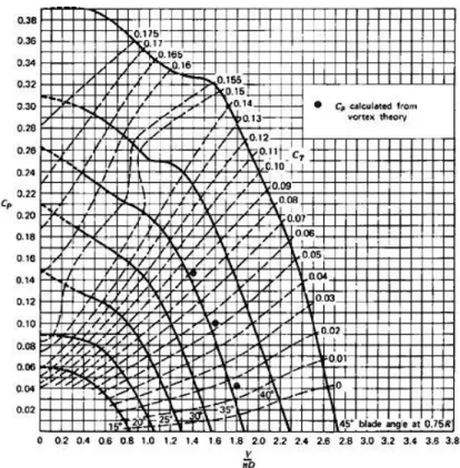
PropSelector is a program that was designed by Brian Robert Gyles [4] which provides as output the performance of two to four blade propellers of model airplanes and is based on the mutual relations of propeller data from NACA’s Technical Note No.698 [5]. There is an extended version of this program called Extended Propselector, which allows input of altitude and provides more output values, such as propeller thrust coefficient, tip Mach number and Pitch angle at 75% of propeller blade radius.

2.3.2 JBLADE

JBLADE is an open-source propeller design and analysis code developed in UBI, by Morgado and Silvestre [7], as part of a PhD thesis at UBI. It uses a modified BEM theory to account for the 3D flow equilibrium. It can estimate the performance curves of a given propeller, after the analysis it shows the results in a graphical interface to make it easier to build and analyze the simulations. The code used in this model is based on David Marten’s QBLADE coupled with André Deperrois’ XFLR5.

(26)

2.3.3 QPROP Propeller/Windmill analysis and design

QPROP is an analysis program, created by professor Mark J. Drela [8], from Massachusetts Institute of Technology (MIT), which is based on a theoretical aerodynamic formulation that uses an extension of the classical blade-element/vortex formulation, as explained in the document [9], shows as output the analysis of the performance of a propeller-motor combination.

The formulation is based on an extended version of the blade-element/vortex method. This extension, implemented by Larrabee [10], is in the correct accounting of the propeller’s self-induction, making QPROP accurate for very high disk loadings [11].

2.3.4 XROTOR

XROTOR is a program that is mostly used for design and analysis of ducted and free-tip propellers. It contains some menu-driven routines that perform a variety of functions such as: designing a minimum induced loss rotor; prompted input of an arbitrary rotor geometry; the modification of a rotor’s geometry; optimization of a rotor for minimum induced loss; analysis of a rotor’s performance with a lot of operating parameters; incoming slipstream effects; multi-point parameter display; structural analysis and corrections for twist under load; dB noise predictions; interpolation of geometry to a radius of interest; plotting of the results of analysis. XROTOR was developed by Drela [12], that is why the theoretical formulation of this software is almost the same as QPROP, the modification is that QPROP is more geared for doing parameter sweeps and coupling to motors while XROTOR is used for the design and analysis of ducted and free-tip propellers.

The code has been written carefully to safely protect the program from unintended crashes [13], but it is always easy to input determined values which will result in an impossible analysis problem. The mathematical model is incapable of handling flows such as the reverse far-slipstream velocity, this can happen due to the self-deforming wake algorithm being touchy if a high windmill disk loading is combined with low advance ratios. There is, however, an option to disable the self-deforming wake algorithm, but the accuracy of the results might be affected.

2.4 Experimental Studies

Compared to the vast documentation about propeller performance for full-scale airplanes, data on propellers at LRN is scarce. In this section some of the studies conducted on propellers at LRN to date, and the description of the wind tunnels used in each research are shown to better understand some variations in results due to wind tunnel design differences.

(27)

2.4.1 UIUC Propeller Database

Researchers like Brandt, Selig, Ananda and Deters conducted tests on various small propellers, to counteract this lack of documentation on propellers at LRN. Brandt [1] conducted tests on 79 propellers, where almost all of these propellers had a diameter ranging from 9 to 11 inches. These propellers were from different brands: Aeronaut, APC, Graupner, GWS, Kavon, Kyosho, Master Airscrew, Rev up and Zingali. Deters [14] conducted another study, where two types of propellers were tested, namely from the brands: APC, Crazyflie, E-Flite, GWS, KP, Micro Invent, Plantraco, Union and Vapor and ones that have been have been 3D-printed, named: DA4002, DA4022, DA4052 and NR640.

These tests were performed in the UIUC subsonic wind tunnel. The wind tunnel is an open-return type with a 7.5:1 contraction ration. The rectangular test section is nominally 0.853 x 1.219 m in cross section and 2.438 m long. Over the length of the test section, the width increases by approximately 0.0127 m to account for boundary-layer growth along the tunnel sidewalls. Test section speeds are variable up to 71.53 m/s via a 93.25 kW AC motor connected to a five-bladed fan. For the tests presented in reference [1], the maximum tunnel speed used was 24.38 m/s. To ensure good flow quality in the test section, the wind-tunnel settling chamber contains a 0.1016 m thick honeycomb in addition to four anti-turbulence screens.

2.4.2 Department of Aerospace Sciences at UBI

Some information regarding the wind tunnel at UBI [15]:

• The DCA’s wind tunnel is located in the Aerodynamics and Propulsion Laboratory in the DCA at UBI, Covilhã, Castelo Branco, built by EreME;

• This tunnel works with an AC motor with variable speed, with a power rating of 15kW at 970 RPM. Connected to this motor’s shaft there is an axial ventilator with 1.2 m diameter;

• The rectangular test section is 0.8 x 0.8 m in cross-section and 1.5 m long;

• The maximum speed inside the test section, in normal conditions, is about 30 m/s; • The wind-tunnel settling chamber contains a 2 x 2 m honeycomb structure in stainless

steel. The diffuser has a rectangular cross-section at the entrance and a circular exit with a diameter of 1.2 m.

Since 2014 this wind tunnel has its own Low Reynolds Number Propeller Performance Test Rig developed by PhD student Pedro Alves [16]. Prior to this setup the laboratory already had a thrust measuring mechanism developed in 2011 by Ricardo Salas [17]. The test rig was designed to collect data of propellers with a diameter between 6 to 14 inches, operating at Reynolds number between 30,000 to 300,000 (based on chord at 3/4 of the blade radius). It consists on a T-shaped pendulum, resembling the same concept implemented by UIUC. It was designed to have minimum complexity in order to ensure minimal disturbances to the flow [18].

(28)

The validation of this experimental setup included tests on different propellers such as: APC 11x5.5 Thin Electric and APC 10x4.7 Slow Flyer. Besides this validation procedure Alves also conducted tests on propellers which performance was not catalogued: 13x8 Aeronaut Carbon Electric and 12x8 Aeronaut Carbon Electric.

Figure 4 - Schematic of the Wind Tunnel at UBI.

2.2 Surrogate Models

Surrogate models, or metamodels, are compact scalable analytic models that estimate the results of complex tests, based on a limited set of data obtained from experimentation. These are also called response surface models (RSM), emulators, auxiliary models, repro-models, etc. Surrogate models are a cheaper and easier solution for a test or simulation that is expensive or complex to complete because most design problems require complex experiments or simulations to evaluate certain parameters. The main goal of surrogate modeling is to achieve optimal design while reducing the number of design iterations, lowering the costs and improving overall quality. This is possible by going through a process known as curve fitting or function approximation.

2.4.3 Curve fitting methods

A curve fitting method is the process of constructing a curve that best fits a series of data points. It can be solved through interpolation, or “smoothing” which creates a mathematical function that approximately fits the data. To explain these methods in this research, references [19] and [20] were used.

(29)

2.4.3.1 Lagrange Interpolating Polynomials

This method, named after Joseph Louis Lagrange, was already used by Isaac Newton before, but it appears to have been published for the first time in 1779 by Edward Waring. Lagrange worked extensively on this subject but only published later in 1795 [20].

Let 𝑓 be a function whose values are given by 𝑛 + 1 distinct numbers, 𝑥0, 𝑥1, … , 𝑥𝑛. There is a

𝑃(𝑥) polynomial with a maximum degree of 𝑛 with:

𝑓(𝑥𝑘) = 𝑃(𝑥𝑘), for each 𝑘 = 0, 1, … , 𝑛. (2.8) which is given by 𝑃(𝑥) = 𝑓(𝑥0)𝐿𝑛,0(𝑥) + ⋯ + 𝑓(𝑥𝑛)𝐿𝑛(𝑥) = ∑ 𝑓(𝑥𝑘)𝐿𝑘(𝑥) 𝑛 𝑘=0 (2.9)

where, for each 𝑘 = 0, 1, … , 𝑛,

𝐿𝑘(𝑥) = ∏ 𝑥 − 𝑥𝑖 𝑥𝑘− 𝑥𝑖 𝑛 𝑖=0 𝑖≠𝑘 (2.10)

2.4.3.2 Newton Interpolation Polynomial

The Newton Interpolation Polynomial utilizes divided differences to generate a polynomial based on a given set of points.

Let 𝑓 be a function defined in the interval [𝑎, 𝑏] and 𝑥0, 𝑥1, … , 𝑥𝑛 distinct points in between 𝑎

and 𝑏.

𝑓[𝑥𝑖, 𝑥𝑖+1, … , 𝑥𝑖+𝑘] =

𝑓[𝑥𝑖+1, 𝑥𝑖+2, … , 𝑥𝑖+𝑘] − 𝑓[𝑥𝑖, 𝑥𝑖+1, … , 𝑥𝑖+𝑘−1]

𝑥𝑖+𝑘− 𝑥𝑖

(2.11)

The equation set above is the definition of divided difference. Setting as 𝑓𝑖,𝑖+𝑗 the divided difference 𝑓[𝑥𝑖, 𝑥𝑖+1, … , 𝑥𝑖+𝑗].

(30)

Figure 5 - Divided Difference table [19].

From this table, the Newton’s Interpolation Polynomial can be created:

𝑝𝑛(𝑥) = 𝑓(𝑥0) + 𝑓0,1(𝑥 − 𝑥0) + 𝑓0,1,2(𝑥 − 𝑥0)(𝑥 − 𝑥1) + 𝑓0,…,3(𝑥 − 𝑥0)(𝑥 − 𝑥1)(𝑥 − 𝑥2)

+ ⋯ + 𝑓0,…,𝑛(𝑥 − 𝑥0) … (𝑥 − 𝑥𝑛−1)

(2.12)

2.4.3.3 Least Squares Method

A popular curve fitting method is the Linear Least Squares Method (LSQ), which fits the data to minimize the sum of squared residuals:

𝑟𝑖= 𝑦𝑖− 𝑝(𝑥𝑖) (2.13)

𝑆 = ∑ 𝑟𝑖2 𝑛+1

𝑖=1

(2.14)

The least square method (LSQ) is probably the most popular technique in statistics. This is due to several factors. First, most common estimators can be casted within this framework. For example, the mean of a distribution is the value that minimizes the sum of squared deviations of the scores. Second, using squares makes LSQ mathematically very tractable because the Pythagorean theorem indicates that, when the error is independent of an estimated quantity, one can add the squared error and the squared estimated quantity. Third, the mathematical tools and algorithms involved in LSQ (derivatives, eigen-decomposition, singular value decomposition) have been well studied for a relatively long time [21].

(31)

Chapter 3

Methodology

3.1 Experimental procedure

The experimental setup was created by Alves [16] in 2014. It consists of three subsystems, the Propeller Balance, Signal Conditioners and the Data Acquisitions System.

Figure 6 - Experimental Setup designed by Alves [16].

3.1.1 Thrust and Torque Measurements

The thrust load cell used is the CELTRON STC Load cell having a maximum capacity of 100N and the FN3148 manufactured by FGP Sensors & Instrumentation having a maximum capacity of 50N, the two cells must be changed because of the wide variety of propellers’ diameters being tested, thus the error measured is smaller. To test the propellers 13x4, 13x10, 14x10, 15x6, 15x10, 16x10, 18x8, 20x8 and 20x15, all Thin Electric from APC, the 100N load cell was used. Only one propeller, the 7x4, needed to be tested with the 50N cell.

The torque produced by the propeller is measured by a RTS-200 reaction torque transducer made by Transducer Techniques according to the torque level of the propeller being tested.

(32)

Both cells (thrust and torque) are connected to a high precision strain gauge converter from

mantracourt, model SCB-68, that converts a strain gauge sensor input to a digital serial output.

3.1.2 Propeller Speed Measurement

The propeller rotational speed is measured by a Fairchild Semiconductor QRD1114 photo-reflector, that counts the number of revolutions of the output shaft in a fixed time interval (0.75s), resulting in an accuracy of ± 0.5Rev/0.75s.

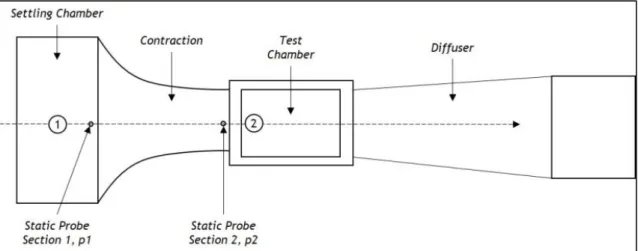
3.1.3 Freestream Velocity Measurement

The freestream velocity is measured with a differential pressure transducer, an absolute pressure transducer, and a thermocouple. This measuring mechanism uses two static pressure ports, one placed in the tunnel settling chamber and the other one at the test chamber, at the end of the contraction. The pressure outside of the tunnel is measured with an absolute pressure transducer made by Freescale Semiconductor model MPXA4115A and the local temperature is measured with a National Instruments LM335 thermocouple located at the inlet of the wind tunnel.

3.1.4 Test Methodology

For the dynamic tests, where 𝐽 > 0, the propeller rotational speed is fixed, and the wind tunnel’s freestream velocity is increased from 4 m/s to 28 m/s in 1 m/s increments, the automatic test has to be stopped once the thrust value reaches 0, because the propeller enters the windmill break state. When testing at lower rotational speeds, the increments have to be in 0.5 m/s in order to acquire more data points within these rotational speeds. At each measured freestream velocity, the thrust and torque generated by the propeller are measured, along with ambient pressure and temperature.

By executing the Labview® data acquisition and reduction software, the procedure of data collection begins. This is followed by putting the program to run test condition. The control software speeds up the motor until it reaches the predefined propeller rotational speed by the user. The test procedure is as explained in reference [16], the only difference being the convergence criteria:

Table 1 - Convergence criteria to achieve wind tunnel freestream speed and propeller’s RPM steady.

Criteria

|𝑅𝑃𝑀 − 𝑅𝑃𝑀𝑡𝑎𝑟𝑔𝑒𝑡| ≤ 10 𝑅𝑃𝑀 |𝑉 − 𝑉𝑡𝑎𝑟𝑔𝑒𝑡| ≤ 0.20 𝑚/𝑠

(33)

When both convergence criteria are met, 200 points are measured at the current freestream velocity and averaged to create a single point, it then proceeds to increase the wind tunnel rotational speed to the next velocity. After a test, all the data points acquired are written in a .txt file by clicking the “Write File” button.

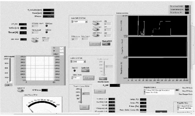
Figure 7 - Data acquisition program interface.

In Figure 7 is displayed the interface of the data acquisition program, where charts show thrust and torque readings over time, readings of propeller’s rotational speed and wind tunnel rotational speed, the thrust and torque measured by the load cells, the convergence points counter, the throttle value for propeller and wind tunnel rotational speed (automatic) and measurements of voltages, pressure and temperature.

3.2 Data reduction

The data obtained through the instruments shown in subsection 3.1 are the measured variables, of thrust, torque, freestream velocity, rotational speed, static pressure, atmospheric pressure and temperature. With the acquired measurements, the calculated variables can be obtained. Power, P, in W, is calculated with n and Q:

(34)

The Patm, Tatm and the air constant, R, 287 J·kg-1·K-1 are used to calculate the air density, 𝜌, in

kg/m3_:

𝜌 = 𝑃𝑎𝑡𝑚 𝑅𝑇𝑎𝑡𝑚

(3.2)

Advance ratio, J, is calculated with V and n: 𝐽 = 𝑉

𝑛𝐷 (3.3)

Thrust coefficient, 𝐶𝑇 and power coefficient 𝐶𝑃 are calculated with the respective parameters

T and P: 𝐶𝑇 = 𝑇 𝜌𝑛2_𝐷4 (3.4) 𝐶𝑃= 𝑃 𝜌𝑛3_𝐷5 (3.5)

Finally, the propeller efficiency is calculated with the variables of 𝐶𝑇 and 𝐶𝑃:

𝜂 =𝐽𝐶𝑇 𝐶𝑃

(3.6)

After the calculation of each individual parameter, 𝐶𝑃 and 𝜂 are plotted against J. Upon

observing the different behavior of all dispersions, all the power coefficient and propeller efficiency points were divided by the natural logarithm of the respective propeller rotational speed at which they were tested, therefore implicitly including the Reynolds number to the calculations since it varies with propeller RPM:

𝐶𝑃

ln(𝑁) ; 𝜂 ln(𝑁)

To simplify the terminology, from now on, these terms will be addressed as: 𝐶𝑃

ln(𝑁)= 𝐶𝑃𝑟 (3.7)

𝜂

ln(𝑁)= 𝜂𝑟 (3.8) where the subscripted r stands for “reduced”.

(35)

The result of this reduction displayed in Figure 8 and Figure 9, where an example is shown for the APC Thin Electric 10x7 propeller, is that the data shows lesser dispersion when divided by ln (𝑁). It should be pointed out that this effect is observable in all the tested propellers’ performance curves. The data reduction is repeated for all the tested propellers.

(36)

Figure 9 - Example of data points of 𝜂 and 𝜂𝑟.

Since the curves have different sizes, but similar forms, in order to compare these curves, to come up with a model that can approximate the values of 𝐶𝑃 and 𝜂 accurately, the next step is

(37)

procedure is done by using the MATLAB® “Curve Fitting Tool” to create a fitting function of 𝐶𝑃𝑟

and 𝜂𝑟 plotted against J, as this tool also displays the coefficients of said curve fits, it is possible

to calculate the values of 𝐶𝑃𝑟0 and 𝜂𝑟𝑚𝑎𝑥. The maximum value of advance ratio, Jmax, is also

retrieved from the function of 𝜂𝑟 as propeller efficiency reaches the value of 0 before the

power coefficient, and J is then divided by Jmax.

𝐶𝑃𝑟 𝐶𝑃𝑟0 ( 𝐽 𝐽𝑚𝑎𝑥 ) (3.9) 𝜂𝑟 𝜂𝑟𝑚𝑎𝑥 ( 𝐽 𝐽𝑚𝑎𝑥 ) (3.10)

After this step, all the propeller performance curves have practically the same limits in the x-axis and the y-x-axis. The curve fitting procedure is the next step to construct an analytical model.

3.3 Least Squares Method

For the nth degree polynomial and a set of n+1 data points [22]:

𝑝𝑛(𝑥𝑖) = 𝑎𝑛𝑥𝑖𝑛+ 𝑎𝑛−1𝑥𝑖𝑛−1… 𝑎0 (3.11)

For curve fit equations which are linear in the coefficients, the n+1 equations can be written in matrix form: [ 𝑝𝑛(𝑥0) 𝑝𝑛(𝑥1) ⋮ 𝑝𝑛(𝑥𝑛+1) ] = [ 𝑥𝑖𝑛 𝑥𝑖𝑛−1 ⋯ 1 𝑥𝑖𝑛 𝑥𝑖𝑛−1 ⋯ 1 ⋮ ⋮ ⋱ ⋮ 𝑥𝑛+1𝑛 𝑥𝑛+1𝑛−1 ⋯ 1] [ 𝑎𝑛 𝑎𝑛−1 ⋮ 𝑎0 ] (3.12)

in short matrix notation:

𝑃 = 𝑋𝑎 (3.13)

Using the least-squares approach to estimate the curve-fit coefficients, a, in matrix notation: 𝑆(𝑎) = (𝑃 − 𝑦)𝑇_{(𝑃 − 𝑦)}

(3.14) = 𝑎𝑇𝑋𝑇𝑋𝑎 − 𝑎𝑇𝑋𝑇𝑦 − 𝑦𝑇𝑋𝑎 + 𝑦𝑇𝑦

(38)

The necessary criterion for minimizing S with respect to the set of curve-fit coefficients, its derivative must be zero.

𝛿𝑆

𝛿𝑎= 0 ↔ 𝑋

𝑇_{𝑋𝑎 = 𝑋}𝑇_{𝑦 (3.15)}

And the unconstrained least-squares estimates for the curve-fit coefficients can be computed from:

𝑎 = [𝑋𝑇_𝑋]−1_𝑋𝑇_{𝑦 (3.16)}

Since the ordinary LSQ fits the best line to data, it does not necessarily mean that the curve fit passes through some points that are explicit, so in this research, it was used the constrained LSQ. To do so, the method of Lagrange multipliers will be applied.

To calculate the coefficients using the constrained LSQ, suppose the curve-fit needs to pass through a certain point (𝑥𝑐, 𝑦𝑐):

𝑦𝑐 = 𝑝(𝑥𝑐) = 𝑎𝑛𝑥𝑐𝑛+ 𝑎𝑛−1𝑥𝑐𝑛−1… 𝑎0 (3.17)

in short matrix notation:

𝑏 = 𝐴𝑎 (3.18)

Like the ordinary LSQ, it is required to minimize the augmented S function (with the Lagrangian):

𝑆(𝑎, 𝜆) = 𝑎𝑇𝑋𝑇𝑋𝑎 − 𝑎𝑇𝑋𝑇𝑦 − 𝑦𝑇𝑋𝑎 + 𝑦𝑇𝑦 + 𝜆𝑇(𝐴𝑎 − 𝑏) (3.19)

Minimizing 𝑆(𝑎, 𝜆) with respect to 𝑎 and maximizing with respect to 𝜆 results in a system of linear equations for the optimum coefficients a* and Lagrange multipliers 𝜆*:

[2𝑋𝑇𝑋 𝐴𝑇 𝐴 0] [ 𝑎∗ 𝜆∗] = ( 2𝑋𝑇_𝑦 𝑏 ) (3.20) If the matrix [𝟐𝑿𝑻𝑿 𝑨𝑻 𝑨 𝟎] is invertible: [𝒂∗ 𝝀∗] = [𝟐𝑿 𝑻_𝑿 _𝑨𝑻 𝑨 𝟎] −𝟏 (𝟐𝑿𝑻𝒚 𝒃 ) (3.21)

(39)

3.4 “Goodness” of fits

This subject describes how well a polynomial approximation, or a statistical model, fits the observed data. There are several ways to identify the “goodness” of the statistical model. Error calculations and the coefficient of determination are some of these methods, explained in subsections 3.4.1 and 3.4.3. To better understand the distance between the data points and the model is an explanation on standard deviation in subsection 3.4.2.

3.4.1 Statistical Error

Often used in validation of linear regressions, the absolute error is the difference between the observed value 𝑦𝑖 at a determined 𝑥𝑖 value, and the model’s prediction, 𝑓𝑖 at the same abscissa.

The absolute error can be calculated through:

𝑒𝑖= |𝑦𝑖− 𝑓𝑖| (3.22)

The relative error can be calculated with the difference between the observed value and the predicted value, divided by the observed value:

𝛿 =|𝑦𝑖− 𝑓𝑖| 𝑦𝑖

(100) =𝑒𝑖

𝑦𝑖(100) (3.23)

The mean relative error (MRE) is also used to evaluate the model and can be calculated as follows (N is the total number of points in the data set):

𝑀𝑅𝐸 =∑𝛿𝑖 𝑁

3.4.2 Standard Deviation

The standard deviation (𝜎) is used to quantify the dispersion of a set of data values. It can be calculated by:

𝜎 = √∑(𝑦𝑖− 𝑓𝑖)

2

𝑁 (3.24)

where 𝜎, represents the standard deviation, 𝑦𝑖 is the measured value and 𝑓𝑖 is the estimated

value.

Lower values of 𝜎 indicate that the data points tend to be close to the model’s prediction, and higher values indicates that the points are farther from the model’s prediction.

(40)

3.4.3 Coefficient of Determination

In regression validation the coefficient of determination is the proportion of the variance in the dependent variable that is predictable from the independent variables. It is calculated with the division of the residual sum of squares with the total sum of squares:

𝑅2_{= 1 −}∑(𝑦𝑖− 𝑓𝑖) 2

∑(𝑦𝑖− 𝑦̅)2

(3.25)

Its value can range from 0 to 1, with a value of 0 meaning the statistical model is not well defined at all, and a value of 1 meaning the statistical model perfectly fits the data.

Typically, anything above 𝑅2_{> 0.7 is considered a very good fit, but it all depends on the}

(41)

Chapter 4

Results and discussion

In this section, the experimental data will be analyzed in order to separate the different 𝐶𝑃

and 𝜂 plots into groups with a common variable, to create a multivariable plot, using regression methods, that describes how the performance parameters behave when plotted against J and a common variable. The results of this analysis will be verified with the measurements from UIUC.

A test will be conducted with the analytical model, to see if the estimated performance curves match the experimental data acquired at UBI. Afterwards, this experimental data will be used to further develop the analytical model, and the updated model will be verified with the measurements from both UIUC and UBI.

4.1 Experimental data

The first step to construct the analytical model is to acquire the data. The analytical model has been constructed with data from the UIUC Propeller Database [2], namely the APC Thin Electric Propellers with the following dimensions: 8x4, 8x6, 8x8, 9x4.5, 9x6, 9x7.5, 9x9, 10x5, 10x7, 11x5.5, 11x7, 11x8, 11x8.5, 11x10, 14x12, 17x12, 19x12. The measurements include thrust and torque coefficient data over a range of advance ratios for specific RPMs. Including some measurements that were taken in static conditions for a few specific RPMs.

The data retrieved from the database includes the measurements of power coefficient, 𝐶𝑃

which is obtained from the measured torque coefficient and advance ratio, and the propeller efficiency, which is obtained from the calculated 𝐶𝑃, and the measured thrust and advance

ratio.

For the validation procedure, tests at the wind tunnel at UBI were conducted, by using the experimental setup created by Alves [16]. The propellers that were tested during the execution of this work are also the same brand and type, APC Thin Electric Propellers, and the dimensions are: 7x4, 13x4, 13x10, 14x10, 15x6, 15x10, 16x10, 18x8, 20x8, 20x15.

(42)

4.2 Curve fitting

4.2.1 Power Coefficient

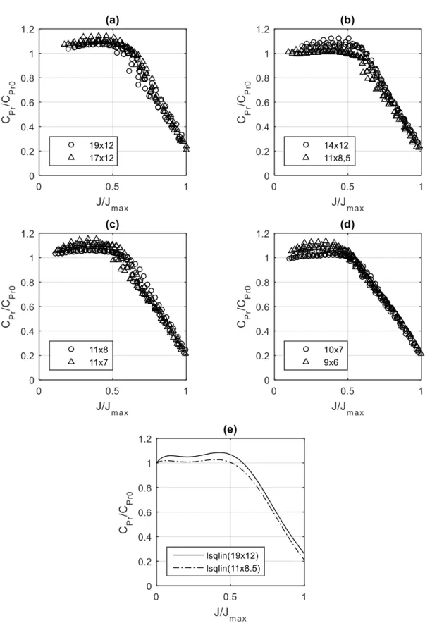
Through analysis of all the data points after reduction, three different behaviors were observed, so the plots were separated into three segments. The first segment (Figure 10) contains the plots of data points corresponding to one behavior that is seen when the propeller’s 𝑝

𝐷 ratio is 0.5. In Figure 11 and Figure 12 are shown the remaining two behaviors that

are observed when the same ratio is not equal to 0.5.

Figure 10 - Dispersion for propellers with 𝑝

𝐷 ratio of 0.5 (a and b) and the results of lsqlin function in MATLAB® (c).

(43)

Figure 11 - 1 of 2 different behaviors of data for propellers with 𝑝

𝐷 ratio not equal to 0.5 (a, b, c, and d) and the results of lsqlin function in MATLAB® (e).

(44)

Figure 12 - 2 of 2 different behaviors of data for propeller with 𝑝

𝐷 not equal to 0.5 (a, b, c) and the results of lsqlin function in MATLAB® (d).

After different attempts, the conclusion is that the graphs show different behaviors based on the 𝐷+𝑝

CPr0 ratio. Propellers with

𝐷+𝑝

CPr0> 2400 show curves like the ones in Figure 11, and propellers

with 𝐷+𝑝

CPr0< 2400 tend to behave like the ones in

(45)

Table 2 - Values of D, p, 𝐶𝑃𝑟0 and 𝐷+𝑝_C

Pr0 for each propeller with 𝑝 𝐷≠ 0.5 : D [in] p [in] 𝑪𝑷𝒓𝟎 𝑫 + 𝒑 𝑪𝑷𝒓𝟎 8 8 0,013 1194 9 9 0,011 1556 8 6 0,008 1579 9 7,5 0,010 1650 11 10 0,009 2168 9 6 0,005 2636 10 7 0,006 2833 11 8,5 0,007 3000 11 8 0,006 3304 11 7 0,005 3600 14 12 0,007 4000 17 12 0,006 5273 19 12 0,005 6200 When 𝑝

𝐷= 0.5 the only relationship is 𝐶𝑃𝑟0:

Table 3 - Values of D, p and 𝐶𝑃𝑟0 for propeller with 𝑝_𝐷= 0.5.

D [in] p [in] 𝑪𝑷𝒓𝟎

8 4 0,004780

9 4,5 0,004888

10 5 0,004446

11 5,5 0,003555

In Figure 10, Figure 11 and Figure 12 there are various curve fits created using the lsqlin function in MATLAB®, which, based on constrained linear least squares theory creates plots to best fit every data point, while satisfying certain constraints, in this case, when 𝐶𝑃𝑟

CPr0(0) = 1.

Some curves are selected to later calculate a multivariable function to best fit all the data. The results of each curve fit shown in Figure 10, Figure 11 and Figure 12 can be found below.

𝑙𝑠𝑞𝑙𝑖𝑛(9𝑥4.5) = 𝐶𝑃𝑟 𝐶𝑃𝑟0 ( 𝐽 𝐽𝑚𝑎𝑥 ) = 19.6429 ( 𝐽 𝐽𝑚𝑎𝑥 ) 6 − 66.5756 ( 𝐽 𝐽𝑚𝑎𝑥 ) 5 + 87.1678 ( 𝐽 𝐽𝑚𝑎𝑥 ) 4 + 66.1909 ( 𝐽 𝐽𝑚𝑎𝑥 ) 3 − 16.0479 ( 𝐽 𝐽𝑚𝑎𝑥 ) 2 + 1.6430 ( 𝐽 𝐽𝑚𝑎𝑥 ) + 1 (4.1)

(46)

𝑙𝑠𝑞𝑙𝑖𝑛(11𝑥5.5) = 𝐶𝑃𝑟 𝐶𝑃𝑟0 ( 𝐽 𝐽𝑚𝑎𝑥 ) = 18.0768 ( 𝐽 𝐽𝑚𝑎𝑥 ) 6 − 59.3233 ( 𝐽 𝐽𝑚𝑎𝑥 ) 5 + 73.7589 ( 𝐽 𝐽𝑚𝑎𝑥 ) 4 − 41.7846 ( 𝐽 𝐽𝑚𝑎𝑥 ) 3 + 8.5878 ( 𝐽 𝐽𝑚𝑎𝑥 ) 2 − 0.0416 ( 𝐽 𝐽𝑚𝑎𝑥 ) + 1 (4.2) 𝑙𝑠𝑞𝑙𝑖𝑛(19𝑥12) = 𝐶𝑃𝑟 𝐶𝑃𝑟0 ( 𝐽 𝐽𝑚𝑎𝑥 ) = −30.2319 ( 𝐽 𝐽𝑚𝑎𝑥 ) 6 + 100.8076 ( 𝐽 𝐽𝑚𝑎𝑥 ) 5 − 123.1031 ( 𝐽 𝐽𝑚𝑎𝑥 ) 4 + 66.1909 ( 𝐽 𝐽𝑚𝑎𝑥 ) 3 − 16.0479 ( 𝐽 𝐽𝑚𝑎𝑥 ) 2 + 1.6430 ( 𝐽 𝐽𝑚𝑎𝑥 ) + 1 (4.3) 𝑙𝑠𝑞𝑙𝑖𝑛(11𝑥8.5) = 𝐶𝑃𝑟 𝐶𝑃𝑟0 ( 𝐽 𝐽𝑚𝑎𝑥 ) = −17.3040 ( 𝐽 𝐽𝑚𝑎𝑥 ) 6 + 59.3863 ( 𝐽 𝐽𝑚𝑎𝑥 ) 5 − 72.9561 ( 𝐽 𝐽𝑚𝑎𝑥 ) 4 + 37.7072 ( 𝐽 𝐽𝑚𝑎𝑥 ) 3 − 8.3066 ( 𝐽 𝐽𝑚𝑎𝑥 ) 2 + 0.6825 ( 𝐽 𝐽𝑚𝑎𝑥 ) + 1 (4.4) 𝑙𝑠𝑞𝑙𝑖𝑛(11𝑥10) = 𝐶𝑃𝑟 𝐶𝑃𝑟0 ( 𝐽 𝐽𝑚𝑎𝑥 ) = −37.4430 ( 𝐽 𝐽𝑚𝑎𝑥 ) 6 + 128.9251 ( 𝐽 𝐽𝑚𝑎𝑥 ) 5 − 165.2866 ( 𝐽 𝐽𝑚𝑎𝑥 ) 4 + 95.2105 ( 𝐽 𝐽𝑚𝑎𝑥 ) 3 − 23.8601 ( 𝐽 𝐽𝑚𝑎𝑥 ) 2 + 1.6216 ( 𝐽 𝐽𝑚𝑎𝑥 ) + 1 (4.5) 𝑙𝑠𝑞𝑙𝑖𝑛(9𝑥9) = 𝐶𝑃𝑟 𝐶𝑃𝑟0 ( 𝐽 𝐽𝑚𝑎𝑥 ) = −14.1857 ( 𝐽 𝐽𝑚𝑎𝑥 ) 6 + 55.6621 ( 𝐽 𝐽𝑚𝑎𝑥 ) 5 − 78.6270 ( 𝐽 𝐽𝑚𝑎𝑥 ) 4 + 48.6145 ( 𝐽 𝐽𝑚𝑎𝑥 ) 3 − 13.4444 ( 𝐽 𝐽𝑚𝑎𝑥 ) 2 + 1.2284 ( 𝐽 𝐽𝑚𝑎𝑥 ) + 1 (4.6) 𝑙𝑠𝑞𝑙𝑖𝑛(8𝑥8) = 𝐶𝑃𝑟 𝐶𝑃𝑟0 ( 𝐽 𝐽𝑚𝑎𝑥 ) = −9.3172 ( 𝐽 𝐽𝑚𝑎𝑥 ) 6 + 40.4902 ( 𝐽 𝐽𝑚𝑎𝑥 ) 5 − 60.9606 ( 𝐽 𝐽𝑚𝑎𝑥 ) 4 + 38.8674 ( 𝐽 𝐽𝑚𝑎𝑥 ) 3 − 10.3888 ( 𝐽 𝐽𝑚𝑎𝑥 ) 2 + 0.5565 ( 𝐽 𝐽𝑚𝑎𝑥 ) + 1 (4.7)

(47)

To minimize the number of equations when calculating the power coefficient, three functions with two variables were created, one for each behavior shown above:

1. 𝑝 𝐷= 0.5 2. 𝑝 𝐷≠ 0.5 𝑎𝑛𝑑 𝐷+𝑝 CPr0> 2400 3. 𝑝 𝐷≠ 0.5 𝑎𝑛𝑑 𝐷+𝑝 CPr0< 2400

Using the definition of a line applied to case 1.:

𝐶𝑃1= 𝑙𝑠𝑞𝑙𝑖𝑛(9𝑥4.5) + 𝑙𝑠𝑞𝑙𝑖𝑛(11𝑥5.5) − 𝑙𝑠𝑞𝑙𝑖𝑛(9𝑥4.5) 0.00355 − 0.004888 (𝐶𝑃𝑟0− 0.00488) (4.8) = 19.6429 ( 𝐽 𝐽𝑚𝑎𝑥 ) 6 − 66.5756 ( 𝐽 𝐽𝑚𝑎𝑥 ) 5 + 87.1678 − 54.5072 ( 𝐽 𝐽𝑚𝑎𝑥 ) 3 + 15.1975 ( 𝑗 𝑗𝑚á𝑥 ) ( 𝐽 𝐽𝑚𝑎𝑥 ) 2 − 1.7161 ( 𝐽 𝐽𝑚𝑎𝑥 ) − [(𝐶𝑃𝑟0− 0.00488) (−1177.518797 ( 𝐽 𝐽𝑚𝑎𝑥 ) 6 + 5452.857143 ( 𝐽 𝐽𝑚𝑎𝑥 ) 5 − 10081.8797 ( 𝐽 𝐽𝑚𝑎𝑥 ) 4 + 9565.864662 ( 𝐽 𝐽𝑚𝑎𝑥 ) 3 − 4969.699248 ( 𝐽 𝐽𝑚𝑎𝑥 ) 2 + 1259.022556 ( 𝐽 𝐽𝑚𝑎𝑥 ))]

Creates the following plot:

(48)

For case 2: 𝐶𝑃2= 𝑙𝑠𝑞𝑙𝑖𝑛(11𝑥8.5) + 𝑙𝑠𝑞𝑙𝑖𝑛(19𝑥12) − 𝑙𝑠𝑞𝑙𝑖𝑛(11𝑥8.5) 6200 − 3000 ( 𝐷 + 𝑝 𝐶𝑃𝑟0 − 3000) (4.9) = −17.304 ( 𝐽 𝐽𝑚𝑎𝑥 ) 6 + 167.5 ( 𝐽 𝐽𝑚𝑎𝑥 ) 5 − 72.9561 ( 𝐽 𝐽𝑚𝑎𝑥 ) 4 + 37.7072 ( 𝐽 𝐽𝑚𝑎𝑥 ) 3 − 8.3066 ( 𝐽 𝐽𝑚𝑎𝑥 ) 2 + 0.6825 ( 𝐽 𝐽𝑚𝑎𝑥 ) + 1 − [(𝐷 + 𝑝 𝐶𝑃𝑟0 − 3000) (−0.00403996875 ( 𝐽 𝐽𝑚𝑎𝑥 ) + 0.01294415625 ( 𝐽 𝐽𝑚𝑎𝑥 ) 5 − 0.0156709375 ( 𝐽 𝐽𝑚𝑎𝑥 ) 4 + 0.00890115625 ( 𝐽 𝐽𝑚𝑎𝑥 ) 3 − 0.00241915625 ( 𝐽 𝐽𝑚𝑎𝑥 ) 2 + 0.00030015625 ( 𝐽 𝐽𝑚𝑎𝑥 ))]

(49)

and for case 3, it is used the definition of a parabola: 𝐶𝑃3= 𝐶𝑃𝑟 𝐶𝑃𝑟0 ( 𝐽 𝐽𝑚𝑎𝑥 ,𝐷 + 𝑝 𝐶𝑃𝑟0 ) = 𝐴 (𝐷 + 𝑝 𝐶𝑃𝑟0 ) 2 + 𝐵 (𝐷 + 𝑝 𝐶𝑃𝑟0 ) + 𝐶 (4.10) Solving with a system of equations:

{ 𝑙𝑠𝑞𝑙𝑖𝑛(11𝑥10) = 𝐴 (𝐷 + 𝑝 𝐶𝑃𝑟0 ) 2 + 𝐵 (𝐷 + 𝑝 𝐶𝑃𝑟0 ) + 𝐶 𝑙𝑠𝑞𝑙𝑖𝑛(8𝑥8) = 𝐴 (𝐷 + 𝑝 𝐶𝑃𝑟0 ) 2 + 𝐵 (𝐷 + 𝑝 𝐶𝑃𝑟0 ) + 𝐶 𝑙𝑠𝑞𝑙𝑖𝑛(9𝑥9) = 𝐴 (𝐷 + 𝑝 𝐶𝑃𝑟0 ) 2 + 𝐵 (𝐷 + 𝑝 𝐶𝑃𝑟0 ) + 𝐶 (4.11)

Solving for A, B and C results in a final equation 𝐶𝑃3:

𝐶𝑃3= 𝐶𝑃𝑟 𝐶𝑃𝑟0 ( 𝐽 𝐽𝑚𝑎𝑥 ,𝐷 + 𝑝 𝐶𝑃𝑟0 ) = (−0.00002519568556 ( 𝐽 𝐽𝑚𝑎𝑥 ) 6 + 0.00007983583595 ( 𝐽 𝐽𝑚𝑎𝑥 ) 5 − 0.00009522857874 ( 𝐽 𝐽𝑚𝑎𝑥 ) 4 + 0.00005049925633 ( 𝐽 𝐽𝑚𝑎𝑥 ) 3 − 0.000008799029191 ( 𝐽 𝐽𝑚𝑎𝑥 ) 2 ) (𝐷 + 𝑝 𝐶𝑃𝑟0 ) 2 + (0.05582316189 ( 𝐽 𝐽𝑚𝑎𝑥 ) 6 − 0.1775868247 ( 𝐽 𝐽𝑚𝑎𝑥 ) 5 + 0.213017194 ( 𝐽 𝐽𝑚𝑎𝑥 ) 4 − 0.1119150618 ( 𝐽 𝐽𝑚𝑎𝑥 ) 3 + 0.01574791229 ( 𝐽 𝐽𝑚𝑎𝑥 ) 2 + 0.005288737972 ( 𝐽 𝐽𝑚𝑎𝑥 )) (𝐷 + 𝑝 𝐶𝑃𝑟0 ) + (−40.05004857 ( 𝐽 𝐽𝑚𝑎𝑥 ) 6 + 138.711635 ( 𝐽 𝐽𝑚𝑎𝑥 ) 5 − 179.5414078 ( 𝐽 𝐽𝑚𝑎𝑥 ) 4 + 100.5001657 ( 𝐽 𝐽𝑚𝑎𝑥 ) 3 − 16.64743656 ( 𝐽 𝐽𝑚𝑎𝑥 ) 2 − 3.979392749 ( 𝐽 𝐽𝑚𝑎𝑥 ) + 1) (4.12)

(50)

Since both 𝐶𝑃2 and 𝐶𝑃3 depend on the same two variables, 𝐽 𝐽_𝑚𝑎𝑥 and

𝐷+𝑝

C_Pr0 it is possible to plot

both as a piecewise function:

𝐶𝑃2,3 { 𝐶𝑃2( 𝐽 𝐽𝑚𝑎𝑥 ,𝑝 + 𝐷 𝐶𝑃𝑟0 ) , 𝑝 + 𝐷 𝐶𝑃𝑟0 < 2400 𝐶𝑃3( 𝐽 𝐽𝑚𝑎𝑥 ,𝑝 + 𝐷 𝐶𝑃𝑟0 ) , 𝑝 + 𝐷 𝐶𝑃𝑟0 ≥ 2400 (4.13) Figure 14 - 3D plot of 𝐶P2,3.

(51)

4.2.2 Propeller Efficiency

Figure 15 - 1 of 2 behaviors of propeller efficiency when 𝑝 𝐷> 0.9.

Figure 16 - 2 of 2 behaviors of propeller efficiency when 𝑝 𝐷< 0.9.

(52)

The curve fits shown in Figure 15 and Figure 16 have also been created using the lsqlin function from the “Optimization Tool” in MATLAB®. The constraints used in these two cases were:

• 𝜂𝑟 𝜂_{𝑟𝑚𝑎𝑥}(0) = 0; • 𝜂𝑟 𝜂𝑟𝑚𝑎𝑥(1) = 0; • 𝑑( 𝜂𝑟 𝜂𝑟𝑚𝑎𝑥(( 𝐽 𝐽𝑚𝑎𝑥)𝜂_ 𝑚𝑎𝑥)) 𝑑( 𝐽 𝐽𝑚𝑎𝑥) = 0. 𝑙𝑠𝑞𝑙𝑖𝑛 (𝑝 𝐷> 0.9) = −77.1935 ( 𝐽 𝐽𝑚𝑎𝑥 ) 6 + 202.5785 ( 𝐽 𝐽𝑚𝑎𝑥 ) 5 − 196.5373 ( 𝐽 𝐽𝑚𝑎𝑥 ) 4 + 83.3452 ( 𝐽 𝐽𝑚𝑎𝑥 ) 3 − 15.0943 ( 𝐽 𝐽𝑚𝑎𝑥 ) 2 + 2.9014 ( 𝐽 𝐽𝑚𝑎𝑥 ) (4.14) 𝑙𝑠𝑞𝑙𝑖𝑛 (𝑝 𝐷< 0.9) = −29.4085 ( 𝐽 𝐽𝑚𝑎𝑥 ) 6 + 65.2815 ( 𝐽 𝐽𝑚𝑎𝑥 ) 5 − 51.8950 ( 𝐽 𝐽𝑚𝑎𝑥 ) 4 + 16.7248 ( 𝐽 𝐽𝑚𝑎𝑥 ) 3 − 3.3596 ( 𝐽 𝐽𝑚𝑎𝑥 ) 2 + 2.6568 ( 𝐽 𝐽𝑚𝑎𝑥 ) (4.15)

To create a multivariable function that relates the two curve fits represented in Figures 14 and 15, a similar approach to the one used with the power coefficient was used, but this time the second variable introduced is 𝑝

𝐷:

Table 4 - Averages of propellers' 𝑝 𝐷 ratio. Propeller Average 𝑝 𝐷 ratio Propeller 8x4 0.6629263 Propeller 8x6 Propeller 9x4.5 Propeller 9x6 Propeller 9x7.5 Propeller 10x5 Propeller 10x7 Propeller 11x5.5 Propeller 11x7 Propeller 11x8 Propeller 11x8.5 Propeller 14x12 Propeller 17x12 Propeller 19x12 Propeller 8x8 0.9696970 Propeller 9x9 Propeller 11x10

(53)

𝜂𝑟 𝜂𝑟𝑚𝑎𝑥 ( 𝐽 𝐽𝑚𝑎𝑥 ,𝑝 𝐷) = 𝑙𝑠𝑞𝑙𝑖𝑛 (𝑝 𝐷> 0.9) + 𝑙𝑠𝑞𝑙𝑖𝑛 (_𝐷𝑝 < 0.9) − 𝑙𝑠𝑞𝑙𝑖𝑛 (_𝐷𝑝 > 0.9) 0.6629263 − 0.9696970 ( 𝑝 𝐷− 0.9696970) (4.16)

Which resulted in:

Figure 17 - 3D plot of 𝜂1. 𝜂1= 𝜂𝑟 𝜂𝑟𝑚𝑎𝑥 ( 𝐽 𝐽𝑚𝑎𝑥 ,𝑝 𝐷) = −77.1935 ( 𝐽 𝐽𝑚𝑎𝑥 ) 6 + 202.5785 ( 𝐽 𝐽𝑚𝑎𝑥 ) 5 − 196.5373 ( 𝐽 𝐽𝑚𝑎𝑥 ) 4 + 83.3452 ( 𝐽 𝐽𝑚𝑎𝑥 ) 3 − 15.0943 ( 𝐽 𝐽𝑚𝑎𝑥 ) 2 + 2.9014 ( 𝐽 𝐽𝑚𝑎𝑥 ) + (𝑝 𝐷− 0.969697) (−155.7678096 ( 𝐽 𝐽𝑚𝑎𝑥 ) 6 + 447.5557803 ( 𝐽 𝐽𝑚𝑎𝑥 ) 5 − 471.4997228 ( 𝐽 𝐽𝑚𝑎𝑥 ) 4 + 217.1667633 ( 𝐽 𝐽𝑚𝑎𝑥 ) 3 − 38.25234939 ( J Jmax ) 2 + 0.7973382073 ( J Jmax )) (4.17)

(54)

4.2.3 Additional Parameters

In order to calculate the real power coefficient and the propeller efficiency there are still some functions to create, such as: 𝐽𝑚𝑎𝑥(𝐷, 𝑝), 𝐶𝑃𝑟0(𝐷, 𝑝) and 𝜂𝑟𝑚𝑎𝑥(𝐷, 𝑝).

Using MATLAB® application “Curve Fitting Tool”, these two variable plots were created:

Figure 18 - Jmax(D, p).

𝐽𝑚á𝑥(𝐷, 𝑝) = 1.586 − 0.3891𝐷 + 0.3331𝑝 + 0.0323𝐷2− 0.02883𝐷𝑝 − 0.003682𝑝2

(55)

Figure 19 - 𝐶𝑃𝑟0(𝐷, 𝑝).

𝐶𝑃𝑟0(𝐷, 𝑝) = 0.006016 − 0.002697𝐷 + 0.006181𝑝 + 0.0005193𝐷2− 0.001557𝐷𝑝

+ 0.00065𝑝2_{+ 0.00002425𝐷}3_{− 0.0001404𝐷}2_{𝑝 + 0.0002747𝐷𝑝}2

− 0.0001503𝑝3

(56)

Figure 20 - 𝜂𝑟𝑚𝑎𝑥(𝐷, 𝑝).

𝜂𝑟𝑚𝑎𝑥(𝐷, 𝑝) = 0.08772 − 0.00653𝐷 + 0.0005099𝑝 + 0.0001196𝐷2+ 0.00136𝐷𝑝

− 0.0005098𝑝2_{− 0.0000632𝐷}3_{+ 0.0002344𝐷}2_{𝑝 − 0.000376𝐷𝑝}2

+ 0.0001666𝑝3

(57)

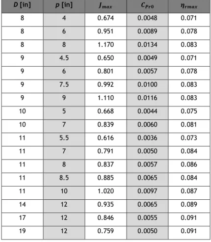
Table 5 - Values of 𝐷, 𝑝, 𝐽𝑚𝑎𝑥, 𝐶𝑃𝑟0 and 𝜂𝑟𝑚𝑎𝑥 used in the plotting of the functions above. D [in] p [in] 𝑱𝒎𝒂𝒙 𝑪𝑷𝒓𝟎 𝜼𝒓𝒎𝒂𝒙 8 4 0.674 0.0048 0.071 8 6 0.951 0.0089 0.078 8 8 1.170 0.0134 0.083 9 4.5 0.650 0.0049 0.071 9 6 0.801 0.0057 0.078 9 7.5 0.992 0.0100 0.083 9 9 1.110 0.0116 0.083 10 5 0.668 0.0044 0.075 10 7 0.839 0.0060 0.081 11 5.5 0.616 0.0036 0.073 11 7 0.791 0.0050 0.084 11 8 0.837 0.0057 0.086 11 8.5 0.885 0.0065 0.084 11 10 1.020 0.0097 0.087 14 12 0.935 0.0065 0.089 17 12 0.846 0.0055 0.091 19 12 0.759 0.0050 0.091

4.3 Validation

To see if the model fits the data accurately, for every propeller within the APC Thin Electric family, tested at UIUC, an estimate of the values for 𝐶𝑃 and 𝜂, for each RPM at which they were

tested, was created. This estimate is represented by the lines in the figures throughout subsection 4.3.1. Alongside these lines, the measurements made at UIUC are also represented for an easier comparison between the model’s prediction, and the measured data.

In subsection 4.3.2, the analytical model will be validated by conducting tests for the APC Thin Electric Propellers with dimensions: 7x4, 13x4, 13x10, 14x10, 15x6, 15x10, 16x10, 18x8, 20x8, 20x15.

The calculated values of 𝐶𝑃 and 𝜂, obtained with the measurements of thrust and torque

coefficients at UBI, will be plotted alongside with the lines created with the analytical model, for each set RPM.

(58)

4.3.1 Comparison with UIUC Propeller Database

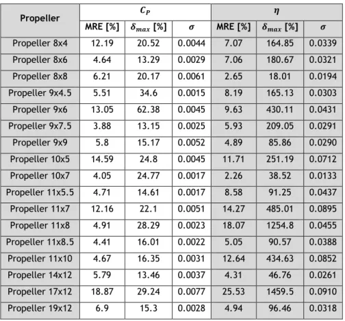
Demonstrated in Table 6 are the results of the mean relative error (MRE) calculations, the maximum relative error, 𝛿𝑚𝑎𝑥 and the standard deviation, 𝜎 measured for each propeller

relatively to the model’s predictions. The measured 𝛿𝑚𝑎𝑥 for 𝜂 are somewhat higher than

expected because of the sharp decline in the curve after reaching peak propeller efficiency.

Table 6 - Mean relative error of the model's predictions for the first model.

Propeller 𝑪𝑷 𝜼 MRE [%] 𝜹𝒎𝒂𝒙 [%] 𝝈 MRE [%] 𝜹𝒎𝒂𝒙 [%] 𝝈 Propeller 8x4 12.19 20.52 0.0044 7.07 164.85 0.0339 Propeller 8x6 4.64 13.29 0.0029 7.06 180.67 0.0321 Propeller 8x8 6.21 20.17 0.0061 2.65 18.01 0.0194 Propeller 9x4.5 5.51 34.6 0.0015 8.19 165.13 0.0303 Propeller 9x6 13.05 62.38 0.0045 9.63 430.11 0.0431 Propeller 9x7.5 3.88 13.15 0.0025 5.93 209.05 0.0291 Propeller 9x9 5.8 15.17 0.0052 4.89 85.86 0.0290 Propeller 10x5 14.59 24.8 0.0045 11.71 251.19 0.0712 Propeller 10x7 4.05 24.77 0.0017 2.26 38.52 0.0133 Propeller 11x5.5 4.71 14.61 0.0017 8.58 91.25 0.0437 Propeller 11x7 12.16 22.1 0.0051 14.27 485.01 0.0895 Propeller 11x8 4.91 28.29 0.0023 18.07 1254.8 0.0455 Propeller 11x8.5 4.41 16.01 0.0022 5.05 90.57 0.0388 Propeller 11x10 4.67 16.35 0.0031 12.64 434.63 0.0852 Propeller 14x12 5.79 13.46 0.0037 4.31 46.76 0.0261 Propeller 17x12 18.87 29.24 0.0077 25.53 1459.5 0.0910 Propeller 19x12 6.9 15.3 0.0028 4.94 96.46 0.0318

(59)

Figure 21 - Propeller Performance comparison with UIUC data for propeller 8x4.

(60)

Figure 24 - Propeller Performance comparison with UIUC data for propeller 9x4.5.

(61)

(62)

(63)

(64)

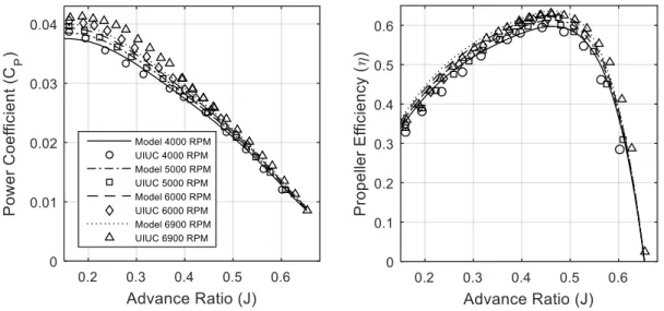
In Figure 21 through Figure 37 the estimates made from the model are displayed, represented by line plots, along with the measurements made at UIUC, in order to examine how the analytical model can estimate the observed values of 𝐶𝑃 and 𝜂. Comparing the different results,

it is seen that:

1. The 𝜂 estimates match the propeller performance data from measurements;

2. The 𝐶𝑃 estimates match the propeller performance data from measurements for

propellers 8x4, 8x6, 8x8, 9x4.5, 9x7.5, 9x9, 10x7, 11x8;

3. The 𝐶𝑃 estimates for propellers 11x7 and 11x10 are the worst matches when compared

with the propeller performance data from measurements for propellers;

4. It is possible to observe that both 𝐶𝑃 and 𝜂, increase with the increase of the propeller

rotational speed. This is a typical behavior for low Reynolds number conditions. Although this increase is more accurate for 𝜂 estimates than the 𝐶𝑃 ones, as observed

(65)

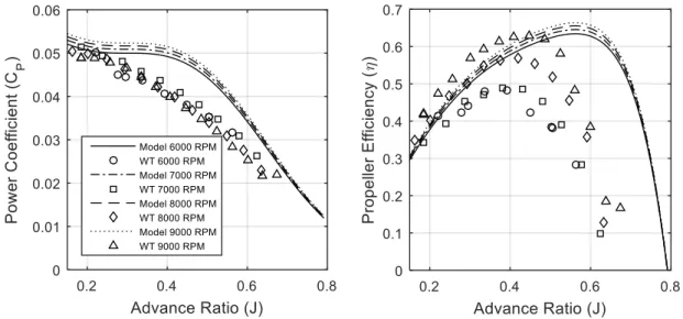
4.3.2 Application of the model to the data acquired at UBI

For this validation, some propellers were tested and compared to the results shown in the model. The propellers used were also from the APC Thin Electric family, 13x4, 13x10, 14x10, 15x6, 15x10, 16x10, 18x8, 20x8, 20x15.

Table 7 - Mean relative error (MRE), 𝛿𝑚𝑎𝑥 and standard deviation of the model's prediction of the propeller's tested at UBI.

Propeller 𝐶𝑃 𝜂 MRE [%] 𝛿𝑚𝑎𝑥 [%] 𝜎 MRE [%] 𝛿𝑚𝑎𝑥 [%] 𝜎 Propeller 7x4 20 42.75 0.0078 52.57 535.89 0.1913 Propeller 13x4 756.07 1061.2 0.0994 61.31 732.76 0.1459 Propeller 13x10 3.20 11.83 0.0015 28.31 404.06 0.1043 Propeller 14x10 8.93 13.32 0.0042 19.25 135.04 0.1149 Propeller 15x6 354.43 1080.6 0.0613 2869.3 159370 0.0958 Propeller 15x10 23.67 31.34 0.0101 23.09 403.54 0.1151 Propeller 16x10 30.23 42.62 0.0108 27.49 196.92 0.1445 Propeller 18x8 234.84 332.88 0.0457 16.25 97.38 0.0798 Propeller 20x8 734.89 971.73 0.1135 40.87 209.96 0.1754 Propeller 20x15 94.40 118.54 0.0353 17.21 67.86 0.0973

As observable in Table 7, the results are not positive for the majority of the propellers measured at UBI. The massive 𝛿𝑚𝑎𝑥 values calculated for propeller efficiency, are due to the sharp decline

observed after peak efficiency is reached.

The results of this application are demonstrated in Figure 38 through Figure 47:

(66)

Figure 39 - Testing of the first model with data from propeller 13x4.

(67)

(68)

Analytical Model for the Performance Curves of a Family of Propellers based on Wind Tunnel Tests

UNIVERSIDADE DA BEIRA INTERIOR

Engenharia