On the monex solutions of backwater problems for uniform open channels

On the monex Solutions of backwater

problems for uniform open channels (*}

by

Prof. P. DE VARENNES E MENDONÇA Chair of General and Agricultural Hydraulics

RESUMO

Começa-se por recordar o estabelecimento da forma mais geral até agora conhecida da equação de Bemoulli para o tratamento unidimensional das cor­ rentes líquidas permanentes, a maneira como dela se deduz a correspondente equação diferencial das curvas de regolfo em canais abertos uniformes e ainda o conceito de valores críticos do escoamento.

Estabelecem-se em seguida fórmulas que, de um modo geral, permitem cal­ cular curvas e volumes de regolfo nesses canais.

Introduzido o conceito de solução monex dum problema de regolfo, mostra-se que fornecem soluções monex as secções transversais rectangular e parabólica larguíssimas, bem como a triangular.

Examinada depois a questão da influência da fórmula de movimento uni­ forme escolhida, indica-se como pode ser unificada a formulação dos problemas de regolfo, seja para canais inclinados, seja para canais horizontais, propondo-se para estes a adopção de um função à qual se atribui o nome de Gagliardi.

Após uma notícia sobre as tábuas das funções de Dupuit e de Gagliardi de interesse para a obtenção de soluções monex usando a fórmula de Chézy, a de Manning e a de Forchheimer, dão-se alguns exemplos numéricos de aplicação.

(*) Paper written in partial fulfilment of the duties inherent to a sabbatical leave begun 16 September 1979 and ending 31 July 1980.

RÊSUMÊ

D’abord on rappelle 1'établissement de la forme la plus générale jusqu’ici connue de 1’équation de Bernoulli pour le traitement unidimensionnel des courants liquides permanents, la manière d’en déduire la correspondante équation diffé- rentielle des courbes de remous en canaux découverts uniformes et aussi le concept de valeurs critiques de 1’écoulement.

On établit ensuite des formules qui, d’une façon générale, permettent de calculer courbes et volumes de remous dans ces canaux.

Après 1’introduction du concept de solution monex d’un problème de remous, on montre que fournissent des Solutions monex les sections transversales rectan- gulaire et parabolique très larges, ainsi que celle triangulaire.

Une fois la question de 1’influence de la formule du mouvement uniforme choisie étant examinée, on indique comment peut être unifiée la formulation des problèmes sur des courbes et des volumes de remous, soit en canaux inclinés, soit en canaux horizontaux, pour ceux-ci l’adoption d’une fonction, à laquelle on attribue le nom de Gagliardi, étant proposée.

Après une notice sur les tables des fonctions de Dupuit et de Gagliardi d’intérêt pour 1’obtention de Solutions monex en employant la formule de Chézy, celle de Manning et celle de Forchheimer, on donne quelques exemples numériques d'application.

SYNOPSIS

To begin with, it is recalled the establishment of the most general form, so far known, of Bernoulli’s équation for dealing one-dimensionally with hydrau- lic steady streams, the way of deducing from it the corresponding differential équation of backwater curves in uniform open channels and also the concept of criticai flow values.

Thereafter formulae that, in a general manner, allow the computation of backwater curves and volumes in such channels are established.

The concept of monex solution of a backwter problem being introduced, it is shown that provide monex Solutions the triangular and also the very wide rectan- gular and parabolic cross-sections.

Next, the question of the influence of the selected uniform flow formula is examined and it is pointed out how the formulation of backwater curves and volumes problems can be unified, either for sloping or for horizontal channels; for the last ones it is proposed the adoption of a function to which the name of Gagliardi is given.

After a notice about the tables of Dupuit and Gagliardi functions relevant for obtaining monex Solutions using Chézy’s, Manning’s and Forchheimer’s for­ mulae, a few numerical examples of application are offered.

1. BernoulWs équation for one-dimensional steady flow.

Consider an isothermal steady stream of a homogenous liquid in a uniform gravitational field. Call Q de discharge, y the weight per unit volume of the liquid and g the acceleration of gravity.

Let us name cross-section of such a stream any section made in it. by a surface that cuts at right angles all its streamlines.

Imagine now that in some region a cross-section £2, of height y, can be traced. A horizontal datum plane having been selected, denote by 2o the elevation of the £1 lowest points and by pa the pressure at one of its highest points, with elevation 2a.

The mean velocity of flow across £l is defined by

where A represents the sectional area. As usual, call a the Coriolis coefficient.

Suppose further that in the neighbourhood of £2 all the stream­ lines are situated on vertical planes n, being parallel those which lie on the same II. More strickly formulated, this hypothesis means to assume that, at all points of n, the osculating planes of the stream­ lines are vertical and that all the streamlines with a common oscu­ lating plane have coincident principal normais. Under these conditions, íl is a ruled surface, having for generating lines the afore-said nor­ mais and upon which the pressure distribution is a function solely of point elevation.

Calling the least angle to the vertical of the intersection of Í2 with any of the n planes, put

2) \ — cos ip •

Assume that ip, and therefore £, has a constant value over Í2, i. e. that are equally inclined the generating lines of the ruled sur­ face £2, the stream cross-section under consideration. Then we shall name £ the Í2 Boudin coefficient.

Consider the intersection of £2 with the II plane which contains one of the £2 lowest points O. Take that straight line as a reference w-axis, with 0 as origin and pointing upwards. It will be

3) 2a = 20 + By .

Let p be the pressure at any point of Í2 with elevation

As it is well known, the piezometric head at this point will be higher or lower than that at a point of elevation 2a according as the streamlines allow their concavity to be seen from above or from below:

L V ^ . V»

z + — ^ za + —

T ^ T

Some authors, as for example Chow (1959, p. 30), call these situa- tions respectively of concave and of convex flow.

By means of 3) and 4), the above relation becomes

V ~ Pa

T and so we can write

V ~ P*

5) ln = e ly

---T

with e ^ 1 according to the afore-said condition.

The Jaeger-Manzanares coefficient 3 maY now be defined thus (Mendonça 1972, eq. 19)]:

Consequently, 3» equal to one in the case of straight streamlines, has a value higher or lower than one according as the flow is concave or convex.

When all the above-mentioned hypotheses are satisfied, the total head of the stream at section íí may be written

with 7) a V2 z0 + \y + — +--- , T 20 X = 3^ •

Suppose now that two such cross-sections, 12, and Q>, the first upstream from the second one, can be found. Labelling with the

sub-Scripts 1 and 2 the values pertaining respectively to and f2z, we may write

P&l CL\V \ P&2 0.2^2

8) Zoi + Xi3/i +---b---= z02 + X2y> +---+---+ i/L ,

Y 29 T 2(/

vvhere is the loss of head from ííi to íi2.

That one is the most general form of Bernoulli’s equation, so far known, for dealing one-dimensionally with hydraulic steady flow pro- blems. At first established only for open channels and plane cross- sections (Mendonça 1964a), it was shortly extended to confined flow (Mendonça 1964-1965) and later on to the case in which, as stated, at all points of both cross-sections the streamlines have vertical oscu- lating planes and each one of these sections, though not plane, is a ruled surface of which the generating lines are equally inclined (Men­ donça 1972).

2. Differential equation of the surface profiles for gradually varied steady flow in uni form open channels.

An open channel is named uniform when it has a cylindrical bed all along which the inner roughness is the same.

In such a channel the so-called gradually varied steady flow refers to a liquid stream for which the following hypotheses nearly hold:

a) the stream free surface is isobaric,

b) the streamlines are everywhere almost parallel.

In equation 8) condition a) implies pal — pu.. and so the terms Pai/r and pa2/y may be dropped. Then that equation reduces to

z0i -b Xij/i + ——- = z02 + X22/2 + ——1 + Hh .

2 g 2 g

Assumption b) becomes more and more accurate the lower the streamlines are situated. For this reason, in order that plane sections of the stream may be taken as cross-sections — in the sense explain- ed before — they ought to be made normally to the generating lines of the cylindrical bed or, what is the same thing, perpendicularly to the so-called bottom line.

Take this line, directed in the sense of the flow, as the abscissas a'-axis. Let xx and x2 be the abscissas of sections and fi2, respect- ively, with reference to an arbitrary origin.

Owing to the way the cross-sections are traced, the bottom line angle to the horizon is equal to ip. The channel slope, i. e. its bottom longitudinal slope S0, is defined by

10) S0 ='± sin ip ,

where the upper sign is conventionnally ascribed when the bottom descends in the flow direction and the lower one when it ascends. Positive slopes are also called sustaining and negative ones adverse. Of course, horizontal channels are those for which (p and Sn are zero.

Now we may write

11) »oi — 002 = ± (0Co — a?,) sin Ip = So Ax

where S is the mean energy slope in the reach, of length X = x2 — xu limited by the sections Í2i and f12.

Introducing 11) and 12) into 9), we get and

12

X

H\. = (a?2 — Xi) & = S Ax,

(W.-+ —) - a^i + —) = («o - s)ax 2 g 2 g thas is or else AE 13) if we put Air S„-S

14)

. , aV2 . , a Q2

E = Xy +---= Xy +

2 g 2gA>

a quantity, although improperly, known by the name of specific energy.

When ííi and íl2 are infinitely close, 13) becomes

15) dE

díc = 80 - S ,

in which S obviously means the energy slope or unit loss of head at the section of abscissa x .

Neglecting the variation of a and X, differentiation of 14) with respect to y yields dE ^ a.Q2 dA a.Q2B 16) --- X --- •--- X ■ > dy gA3 d y gA3 where 17) dA d y

denotes the top width, i. e. the breadth of the cross-section at the free surface. If we put 18) Fr = a Q2B \gA* equation 16) becomes 19) dE d y = X (1 -Fr) .

The division of 15) by 19) supplies the most compact form of the differential equation of stream surface longitudinal profiles, com-monly called backwater curves j Mendonça 1964a; for X = 1, Men­ donça 1945, eq. (211,3) ] :

20

)

dy 80-8 S - 80 dx 1(1-Fr) X(Fr- 1)

o. Criticai values.

The subscript k is used hereafter to label the so-called critica] values.

Equation dE/dy = 0, that is

may be looked from two different standpoints.

Consider first a set of steady streams having as a common cross-section. Then, A and B are constants, whereas Q behaves as a parameter the values of which make distinguishable the various streams vvithin the set. The value of Q that satisfies to 21) is the criticai discharge

is the criticai (mean) velocity.

The uniform flow of mean velocity Vk is also named criticai. We shall call Froude number the ratio of V2 to V2k :

this gives meaning to the Symbol Fr adopted in 18) and shows that the criticai condition corresponds to

21) 22) and 23) XgA aB V2 _ Q- aB aQ2B VI A2 ' XgA XgA3 24) Fr = 1 .

From the second viewpoint we consider the set of steady streams having a common discharge Q. Within this new set the parameter is the criticai height yk, since all the other elements of the criticai sec- tion ílk are functions of yk. Equation 21) should now be written

the determination of yk remaining dependent on the shape of ílk. By combining 18) and 25), we get

Following Bakhmeteff (1932, p. 47), let us define criticai slope 7 vvith respect to a depth y as that value the channel slope ought to have in order to make criticai the uniform flow.

Assuming that the mean velocity V is related to the energy slope and to the hydraulic radius R = A/U, where U is the wetted perime- ter, by a monomial formula, which we may write (Mendonça 1945)

the criticai velocity, being the mean velocity of the uniform criticai flow, must be given by

25) _{■^■k _}

O.Q-26)

27)

v, = \Jxie<p Z0

and it will get the value 28)

when the section height is the criticai one, yk .

Then, writing 25) in the form

XsrAk 2 \gAk

Q2 =--- = Ak---,

aBk aBy

we see at once that the following identity holds:

29) Q = AV = Ak ykk .

which, by 27) and 28), yields

or 30)

(t

i.i

ií\sf'v-S Ik\Ak

J

Further on, from 28) and 29), we get

Q' K x r: / <P 0 k Ik and 31) V - «jí CP+2 X^-k

Jf. Computing backwater curves and volumes in general. Jf.l. Sloping channels.

Let us label with the subscript zero the normal values relative to Q, i. e. those assumed at any cross-section when the flow is uniform.

Put (unit height) 32) 33) u = y_ yo Write Ao <p+a _{-3 U0 \ — B} --- e — 0 — = M9 U B n

and 34)

The analytical method for solving backwater problems in uniform open channels called principal by the writer (Mendonça 1964a) is based on the hypothesis that q and r can be supposed to keep constant values all along the reach under consideration.

Equation 27) may be written

where, as in 10), the upper sign refers to sustaining and the lower one to adverse bottom slopes.

From 34), 35) and 36), we get 35)

and so we have

36)

that implies

37) SoC±M*r — 1) = | So| (U r + 1) •

and

38) \(Fr — 1) = wM?'r — a

vvith

39) clQ-Bo

gÀ'u

Observing that from 32) we get

40) dy = y0 dw ,

the introduction of 37) and 38) into 20) yields

41)

Sol 1 + ur

and, to obtain the distance X from fi, to n,, it suffices to integrate:

It is called backater volume, with respect to a given pair of cross- sections, the volume of liquid included in between these sections

(Mendonça 1964c).

The infinitesimal backvvater volume with respect to the sections of abscissas x and x + d# is

43) d-c = A d#

and consequently it depends, not only on u, but also on the section shape.

with Pi and s, constants (i = 1, 2, ... A:), and paying attention to 41), equation 43) may be written

42)

Putting 44)

45) dT = —— 2é V" , 1 V 1 + r* WM,+Si-Ur+,i ,pi --- dw

S„ I 1 + ur

Hence, the backwater volume with respect to the sections íh and fl2 is

/ / » Mi /»M,

46) _{T = ----}1 S V»+s‘ P.1 , d“ - <0 / uq+8i áu \ |So|

i x Ju-, 1 T Mr / u* 1 + Ur I

Since 1964 that the writer has been showing how a certain two- valued diparametric function of the non-negative real variable intro- duces itself quite naturally into many problems of Fluid Mechanics (Mendonça 1964a, 1964c, 1977, 1978). Denoted by D^(w) and defined as follows it has been named Dupuit function in honour to Arsène- Jules-Émile-Juvénal Dupuit: minus branch u < 1 u > 1 47) D"(u) plus branch /»50 + m / uM du D (u) = I ---nV c/,1 +uk Mm _áu ,1 -mn *1.001 WM _du .1 - us UM _áu

For backwater problems, the minus branch pertains to sustaining slopes (S„>0) and the plus branch to adverse slopes (S'„<0).

And so formulae 42) and 46) respectively may be written too:

S„' DTr{Un) ~ DUu,) to DUu,) - DUu,)

1

49)

[

d

r

(u2) -DVHu,)

— O) (**) -U r

50)

Jf.2. Horizontal channels.

When the bed is horizontal, we have f s0=o

I X/=P

and then equation 20) becomes

51)

52)

3

àx = — (Fr - 1) áy . S

We shall call reduced height of the cross-section the ratio

y

u = 2/k

from which we get

53) dy = yk du .

Introducing 26), 30), 52) and 53) into 51), the following form is obtained for the differential equation of backwater curves in hori­ zontal uniform open channels:

The assumed constancy of q and r make 33) and 34) to imply

and

56)

57)

. \ Cp+2 . Cp >

(z)“(S)T-(£)-'

This allows 54) to get the more simple look 33/k

da; =--- (u9 — ur) du ,

of immediate integration:

58) X =

33/^ _{<2+1 r+l g+l r+l}

^ U2 _ U2 j ^ Oi _ Ui ^

q+1 r+l q+1 r+l

In honour to Gagliardi, who suggested its usefulness by studying two particular cases (Gagliardi 1974), we shall call

59)

E. E.

r*Ew v _ u V ‘

CrEMu) —

Ei E,,

the Gagliardi function. Introduced into 58), it yields 32/k

60) X = 32/k r

L

Gr+i (u2) — Gr+X(ui) I •

Equation 44) can also be written

61) A == »,= SP*(^) 'W=S^p,u‘

and so, combining 43) with 57), we find

dx = — 2 y'”‘ P.fci***1 du,

that gives by integration 62) U29+«j+1 Ç + Si + l Vz \ r+Si + 1 / 9+8i+l q + Si + l r+8; +1 Ui * r-f S; + l or rather, using Gagliardi function,

63)

[

9+8. + 1 9+8 . + 1

Gr+ê]+i(u2) — Gr+li+1 (Ui)

(*)• 4

5. What is meant by «monex Solutions».

Formulae 48), 49), 60) and 63) are of a quite general use. But it happens that, in most cases, q and r vary along the reach from íh to Í2.. And so, we must proceed either with estimated mean values of the parameters or by dividing the reach into shorter ones wherein such variation might be neglected. Both these ways can give good results in practice, even though theoretically inaccurate.

However, there are some particular cases in which, not only q, r,

Pi and Si remain constant all along the reach, but also this constancy

is independent of the uniform flow formula that has been chosen, pro- vided it be a monomial one, i. e. vvhatever be the values taken by x> <p and 0 in 27). These are the cases that supply the Solutions we call

monex, i. e. mon(omially) ex(act).

Three have been identified: that of the triangular, and those of the very wide rectangular and parabolic cross-sections. Since the «very wide» assumption can be satisfied only approximately, from a strict viewpoint none but the first of these three cases can effectively be realized.

As it will be seen later, contrariwise to the rectangular and the parabolic sections, the triangular one does not need to be symmetric with respect to an axis perpendicular to its horizontal top line.

(*) Formulae 62) and 63) are other forms of that established in 1964 [Mendonça 1964d, eq. 6)].

6. About the cross-sectional shapes known to provide monex Solutions. 6.1. Very wide rectangular section.

The rectangular shape implies

64 j | B = B0 = Bk = const. I A = By

and the very wide (theoretically infinitely wide) condition means that the

65) U=B

assumption holds (Mendonça 1945, p. 28). From 64) and 65), we get

66) or else = *L = ?L = U By„ y» 67) A Ak U_ uk Then it follows By = y_ Byk yk ?- = ! = Bk 3 68)

and 69) 9+2 Cp +2 A) _e 7 JL = u 0 aJ \u ) _Bk Cp +2 9 Cp+2 A\ ~!T 0 = U 0 ’ aJ \U ) -3

that, by comparison with 33), 34), 55) and 56), yield

70) and 71) <7 = ^-3 cp-4-2 r = —

Furthermore, equations 64) give too

A = By0(~) = By0u = B yk(—) = Byk u ,

y o y*

which, compared to 44) and 61) shows we have in this case

72)

i = 1 Si = Si = 1

Px = P\ = B .

6.2. Very wide parabolic section.

The parabola is assumed to have its axis perpendicular to the section top line, This implies (Mendonça 1945, p. 79)

73) 2 A = — By 3 B _B0__Bi = const.

Moreover, 65) holds under the very wide hypothesis. Then we get 74) or else B U v- - = — = (^-)2 = u B0 U0 By 75) It follows 76) and 77) A„ B0y0 B U Bk uk A By Ak Bkyk Cp +2 (A-\

e

\

A0 ) Cp +2 (A \

_9('

\ Ao ) Cp+2 , (A \

0

Cp+2 (a-\

_TV*

\

Ak J

y«

u y

k

Cp <P+H

I i =

u J B0 Cp cp +:« 0 = u Uk\

T B ““4

K=u \ C7 / cp cp +;i

'

ji

\ 7 = uT”

78) and 79)

So, both 76) and 77) furnish cp+3

q = - 4

On the other hand, from equations 73) we also get

3 3

and, by comparison with 44) and 61),

i = 1 80) Si = s 3 ¥ i 6.5. Triangular section.

As it has already been said, the triangle does not need to be isosceles.

Let Si and 82 be the angles of the sides to the horizon. Then Cj = cot 8i and c? = cot 82 are their slopes. And we have

81)

2

B =■ (c, + c2) y

C7 = (V/l + c?+

\J

1

+ cl)y •

From these equations we get

82)

B U = — = u B„ U o

or else — = u*_Ak 83) B U Bk f/k Then it follows (p+2 cp (A.\ ₀ 3 (Uo \ T B „ \ Ao \ u ) B„ 84) Cp+2 <p <P *2 / A \ ( — (Ei) 0 = u 0 V Ao \U ) and CP +4 co Ia 0

7

\ 7 B u \Ak \u ) Bu 85) cp +4

<p

cp 44 (±)

nr

(El) "e = V Ak, \v )

Equations 84) and 85) imply cp + 4 86) q —---5 0 and cp + 4 87) r = —--- . 0

Finally, the first of equations 81) shows that, in the case of the triangular section, we have

i = 1 Si = sx = 2

Pi = P, = — (c, + c2) . 2

7. Infl-uence of the uniform flow formula.

The results so far obtained confirm the statement that the three named sectional shapes provide exact Solutions whatever be the monomial uniform flow formula selected.

Such a choice has however a very important influence on the final results, since q, r, y0 and 7k depend on x, <p and 0.

This will be stressed by considering three of the more widely used formulae, namely those of Chézy (V = C *J RS), Manning (V =

= R2'3 S1/2/n) and Forchheimer (V = XFRn'7 S0-5) .

In all of them is 0 = 1, and so q and r depend only on <p. Formulae 70), 78) and 86) give for the three sectional shapes q = cp — 1. For­ mulae 71), 79) and 87) are reduced to r=cp-f2=g + 3, r=cp + 3=g + 4 and r=<p+4=g+5, respectively.

Table 1 may then be constructed.

TABLE 1

Values of q and r for Chézy, Manning and Forchheimer formulae

Formula 9 Cross-sectional shape Very wide rectangular Very wide parabolic Triangular Q r Q r q r Chézy 1 0 3 0 4 0 5 4 í 10 í 13 í 16 Manning _{¥ ¥} 3 íT ~3 3 7 2 17 2 22 2 27 Forchheimer — — — 5 5 5 5 5 5 5

Let us now investigate into the dependence of 7k, or rather X//k, on both shape and uniform flow formula.

For 0 = 1, 31) may be written q>+2 X _ XyAk /k

Q2 0?

From 25), we get 1 _ aBk Q2 \9 a*

that, when introduced into 89), yields

90)

<p -i

X ax^k^-k

For the very wide rectangular section, 64) and 65) transform 90) into

91)

X ax cp-i

For the very wide parabolic section, the introduction of 65) and 73) into 90) gives

92)

cp-1 <p-l

y

k

Finally, for the triangular section, by means of 81), 90) becomes

<p X _ ax/1 \<p- h g Ci + c2 93) \J 1 + Cl + \J 1 + cl cp-i 3/k •

Each one of equations 91), 92) and 93) generates different ex- pressions according to the value of cp and the signification of x in the

selected uniform flow formula. In the three of these formulae chosen for exemplifying, the values of 9 are those on Table 1 and x is always solely dependent on roughness, being usually denoted, as it was men- tioned above, by C2 in the Chézy’s formula, by l/n2 in the Manning’s and by \2p in the Forchheimer’s.

8. Unified formulation of backwater curves and volumes problems. 8.1. Sloping channels.

Equations 72), 80) and 88) show that for the three sectional sha- pes under consideration we have i = 1, a fact that allows the unifi- cation of 48) and 49) into the single formula

Combining the afore-said equations with Table 1, Table 2, which gives full meaning to 94), can be constructed. In it

1. e. the backater volume per unit normal breadth, refers to the very

wide sections (rectangular and parabolic).

Another feature common to the cases under study, shown by Table 2, is that M is always non-negative, a condition which simpli- fies the analytic expressions of Dupuit function because, according to the rules given in previous papers (Mendonça 1948 and 1978), the first two items (in the 1978 paper named Gu G2 for S0 > 0 and Hu

H. for S„ < 0) are both zero.

This means that all those expressions to be used for obtaining the monex Solutions may be written as follows:

94) J = —

I 8,

96)

with

a/r

Db/P{u) = y+v- - log. Z + 2 (Lj + Tf)

] = \

l|“ = \

J u = u

97) L.= - cos^±^log. («• - 2 «, cos -^ZL + i) 2 j-K w — cos —-— rp _ 9 . 2 (a + p)j7i b 1 i — 2 sin --- arctan ---sin 2 jiz «<1hc = 0.999 M > 1 —» c = 1.001 and 98) + o/p Db/p(u)

I

_{Y + -7- ~ loge Z} 0

+

b—a— — m

_____2<l; +

tp

b—a — — 2 /=1 m = 50 u = u with 99)

L* = — cos --- ---loge (w2 — 2 w cos ——— + 1)(a+p) (2;-l)u . . , 0 (27-Dtt:

b b w — cos (2;-1)tc (a+p) (2;-1)tc . b T' = 2 sin --- ;--- arctan ---—---' b . (2j—l) tz sin

TABLE 2

Values of K, N, M, and M; in formula 94)

Cross-section Uniform flow N

Distance (J = X) _{Volume (J = Tor Ti)} formula K M, m2 K M, M, Chézy 3 3 0 4 1 Very wide Manning 10 10 1 13 4 rectangular _{3 3} n y» ~3~ ~3 17 17 2 22 7 Forchheimer — — — 5 5 5 5 5 11 3 Chézy 4 4 0 2 ~2 Very wide 13 13 1 2 2 35 11

parabolic Manning ₃ y» ₃ 3 3 2,0 6 6

22 22 2 59 19 Forchheimer — 5 5 5 10 10 Chézy 5 5 0 7 2 Triangular Manning 16 16 1 C1 + C2 3 22 7 3 2 3,0 3 3 27 27 2 37 12 Forchheimer 5 5 5 _' 5 5 In 96) to 99) we set 100) _{w = uv}

and

101)

M = —

N = —

p being obviously the least common denominator of the rational num-

bers M and N.

Examining closely the mies afore-mentioned, the following facts, true for the cases under consideration, are easily disclosed.

The value of Y is determined by

102) P a-0+p a > b > y = -a — b + p a<b Y = 0 . u

Somewhat more elaborated is the determination of Z and m. In 96), i. e. for S0 > 0 (sustaining slopes), m is equal to the greatest whole number less then b/2, and Z may be obtained by

-> Z = I w — 1 \ 103) b uneven b even a + p even -> Z = \w'~ — 1 w — 1 a + p uneven -> Z — w + 1

In 98), i. e. for S0 < 0 (adverse slopes), m is the greatest integer less than (b + l)/2, and Z is given by

104) b uneven b even a + p even a + p uneven -> Z = -> Z = w + 1 1 w'+ 1 -> Z = 1 .

These facts, combined with Table 2, made it quite easy to build the Tables 3, 4 and 5.

TABLE 3

Values to be inserted into 96) and 98) when Chézy formula is selected

Seotion Backwater M a P Z _m So > 0 So < 0 So > 0 So < 0 Curve M, 3 _u M+l Very wide J = X M; 0 3 0 « — 11 1 rectangular Volume M, 4 1 1 . — u- 2 M + l 1 J = "ti M; 1 0 M + l Curve M, 4 u |u-l| 2 Very wide J = X M, 0 0 M + l 1 parabolic Volume M, 11 8 2 - --- M2 5 \w —1| 3 J — Ti Mj 3 0 10 + 1 Curve M, 5 M M+l J = X M; 0 0 1 Triang-ular _{5 1} 1 —11 M + l Volume M, 7 lu» 3 M + l J = T m3 2 0 1 M + l _______

Sorti on Very wide rectangular Very wide parabolic Triangular TABLE 4

Values to be inserted into 96) and 98) when Manning formula is selected

Backwater Z “ So > o So < 0 So < 0 So > 0 Curve J = X M, 10 10 3 u 1 w—1| w + 1 1 4 5 m

2

1 0 l”*-ll Volume Jr = T, M, 13 — w= 2 m5 4 0 [ to — 11 to + 1 Curve J = X M, 13 13 u to —1| 10 + 1 6 M; 1 0 Volume J = Tj M, 35 26 6 2 - — u- 5 |io-l| 10 + 1 1 12 13 M, 11 0 Curve M, 16 _u * II m2 1 16 3 0 | toJ — 11 7 8 Volume J — ~ M, 22 — tts₃ |io-l| _{10 + 1} m2 7 0 110= —11

TABLE 5

Forchheimer formula is selected Values to be inserted into 96) and 98) when

Section Very wide rectangular Backwater M Curve J = X Vblume J — Ti M a b V Y Mj 17 u Mj 2 17 0 1 , M, 22 5 — u3 2 Mj 7 0 M, Very wide parabolic Curve J = X Volume J — X i M, M, So > 0 S o < 0 10 + 1 So > 0 So < 0 l™-1! 10 + 1 10 + 1 22 22 59 Mj Triangular M, Curve J = X M. 44 10 ■u-110-11 10 + 1 19 27 27 Mj Volume J = x I M, 37 12 5 1 . — u- 3 10—1 ' 10 + 1 10 + 1 «0 + 1 10 + 1 10 21 11 22 13

8.2. Horizontal channels.

Paying attention to Table 1 and to equations 72), 80), 88), 91), 92) and 93), and remembering 50), we may unify 60) and 63) by writing

105) GÍMu.) -flSi(ui) K"3 K‘*K\

where K3, K4, K-, and KR mean

106) K, = — , 3 107) K< = — , 2 108) K5 = - —--- ---y' 1 + cj + y/ 1 + cl and 109) lír, = Cl + c2,

the values of x» Elf E2, E3> E4, Er„ En and E7 being given by Tables

TABLE 6

Values to be inserted into 105) for tracing backwater curves

(J = X)

Section Formula X E, e. E, E„ E:> E„

1 e7 Chézy _{c- 1 4} i Very wide ₁ 4 13 4 rectangular Manning n- "3 3 0 *3 Forchheimer _Xf 7 5 22 75 Chézy C= ₁ 5 _{0 1}

Very wide Manning 1 4 16 1 ₀

parabolic n' 3 7 27 2 7 Forchheimer Xf _{5 5“ 5 5} Chézy _{C' 1 6} 0 1 1 4 _{19 1 4} Triangular Manning n- 3 5 0 3 3 7 32 2 7 Forchheimer _Xf 5 ~5~ 5 5

TABLE 7

Values to be inserted into 105) for obtaining backwater volumes

(J = Ti = x/-Bk for the very wide sections; J = t for the triangular one)

Section Formula X Ea e2 e3 e4 e5 Ee e7 Very wide rectangular Chézy C" 2 5 0 2 Manning 1 n2 7 3 16 3 73 Forchheimer Xf2 12 5 27 5 12 5 Very wide parabolic Chézy _cr- 5₂ 13₂ í 0 2 Manning í n-17 6 41 6 4 3 7 3 Forchheimer _Xf2 29₁₀ 69₁₀ 7₅ 12 5 Triangular Chézy _cr 3 8 0 í 2 3 Manning í n2 10 3 25 3 4 3 7 3 10 3 Forchheimer _X2f 17 5 42 5 7 5 12 ~5~ 17 5

9. About the numerical tables of Dupuit function for solving back­ water problems with monex Solutions.

9.1. Chézy formula.

The combination «very wide rectangular section plus Chézy for­ mula» is the classical one. The most detailed table available for compu- ting backwater curves was given in a paper (Mendonça 1964b) that also contains a notice of those published before.

For the same combination, but for computing backwater volumes., the first published tables have been included into a set intended to solve problems referring to rectangular channels of any width (Men­ donça 1964e).

It has been recently found that such combination, although not quite satisfactory for turbulent flow (owing to variation of C and a), is absolutely accurate for the laminar flow of Newtonian liquids (because then that variation does not take place); at the same time, it became clear that — mainly in the case of shallow streams located in Zone 3 of Boudin-Bakhmeteff — those first published tables, with only three decimal places, are somewhat inadequate, so that new tables, with 5 and 6 decimal places respectively for sustaining and adverse sloping channels, and more detailed, have been added (Men­ donça 1977).

Besides, for the afore-said combination, the analytical expressions of Dupuit function are simple enough to allow the direct use of any of the many models of electronic pocket «scientific» calculators so popular nowadays.

Tables for computing backwater curves in very wide parabolic and in triangular channels with sustaining slopes, Chézy formula being adopted, were first published respectively by Tolkmitt (1898) and by Puppini (1911).

More accurate tables for these last cases, including adverse slopes, and for many others, are contained in a still unpublished work (Men­ donça unpubl.), where all of them correspond to the following de- scription: _ M Dn (u), 4 dec. u = 0(0.02)0.64(0.01)0.85(0.005)0.95(0.002)0.996(0.001) 0.999; 1.001 (0.001) 1.006 (0.002) 1.05 (0.005) 1.11 (0.01) 1.3 (0.02)1.4(0.05)1.7(0.1)2.2(0.2)4(0.5)6(1)15(5)20(10)30 (20)50; oo ; + .M DN(w), 4 dec. u = 0(0.2)1.4(0.05)1.7(0.1)2.2(0.2)3(0.5)6(1)10(5)20(10) 30(20)50; oo .

Among them are those of D\(u), D^2(u) and D2(u). From these and in the same order, equation

a-6+p a-b Hl) ua/!'áu 1 T pu a—b+p ± u p du 1 + ub'p

allows one to deduce the values of D' {u), D\y*(u) and D\(u), so that it is covered all the field taken into account in Table 3.

9.2. Manning formula.

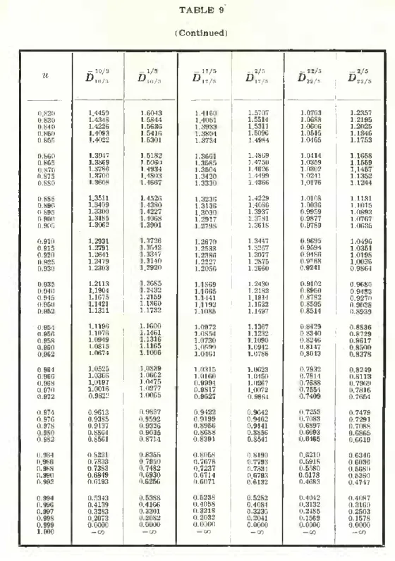
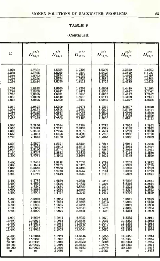
The first author to solve correctly the problem of computing backwater curves in very wide rectangular channels using Manning formula was Supino (1934)(#), whose paper contains short tables of D^(u) for 1 and of D^ÍO) — D^(m). Its values are written with 5 decimal places, but only the first two are reliable. Organized according to scheme 110) and intended for inclusion in the unpublished book mentioned above, correct tables of D^{u) and -DJS/I (®0 were computed by the writer from July to December 1964. They are reproduced in Table 9, placed at the end of this paper.

The problem was recently retaken by Gagliardi (1974) (**), who also gave a correct treatment to the case of the triangular section. His paper contains tables of functions which differ from

^ ^,5/5(“) by constants (***) and that may therefore be put on their places into 94). Writing on the lcft members the symbols used by Gagliardi, those functions are namely

(*) Supino refers to Manning-Strickler formula. A historically better name is however Gauckler-Strickler formula (Mendonça 1945, p. 9-10).

(**) Gagliardi, an Italian engineer, attributed the original integration to Gunder (1942), thus quite surprisingly ignoring the priority of his distinguished compatriote Prof. Giulio Supino.

(***) In the minus branches, these constants are not the same for u < 1 and u > 1, a fact that, of course, is irrelevant.

b(x) = (w) + const.,

ío(x) = D^(u) + const., c(x) = DW(u) - £;;/»(0) Eo(xj = - flv;(u) + í» v;(0) b(x) = + const., (x) = D^u) + const., c(x) =ii>;#(u) -ó;«/»(0) , «.(x) =-c,;';w +D,;/;(0) .

AI1 these tables give the functions values with only three decimal places and for the following intervals and ranges of the argument (*):

0(0.02) 0.6 (0.01 )0.95 (0.005) 1.02 (0.01) 1.2 (0.02) 1.5 (0.05) 2 (0.1)3(0.5)5(1)10(10)20.

For the other cases listed in Table 3 no published or unpublished tables are known to be available by now (**).

9.3. Forchheimer}s and other uniform flow formulae.

By following the rules given above, all the other cases of Dupuit function relative to the monex Solutions can easily be tabulated by anyone who has at his disposal a digital Computer powerful enough. Such a task the writer leaves to the interested reader.

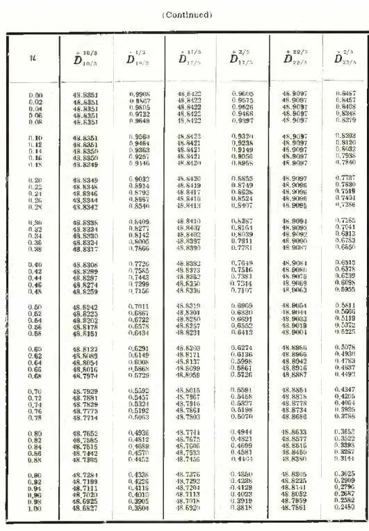
Nevertheless, for the sake of exemplifying the use of Forchhei- mer formula (Section 11), tables of jD^J, DJJ/J and ZM/J,

(*) For the 4 last named functions (Gagliardi 1974, Tabella 2), certainly by misprint, the line corresponding to the value 0.38 of tbe argument has been omitted. It can be easily inferred from Tabella 1 of the same paper: b(0.38) =

= c(0.38) = 0.000, \p0(0.38) = - 0.207, e«(0.38) = 0.206.

(*■*) The paper of Rastrelli (1937) about the case of channels with sustaining slope and very wide parabolic section is unfortunately marred by an error committed still at the establishment of the surface profiles differential equation: from A = 2By/3 the author deduced àA/áy = 2B/3, overlooking the relation, that he correctly wrote two lines below, B = B„-^y/y0 .

picked out from Mendonça (unpubl.), axe given at the end of this paper (Table 9).

For the case of backwater curves in very vvide rectangular chan- nels with sustaining slopes, Forchheimer’s and also one of the Grõger formulae were chosen by Kozeny (1924, 1928). His tables (Weyrauch 1930, p. 248; Forchheimer 1935, p. 245) are however quite rudimentary and unreliable (Mendonça 1945, p. 64).

10. About the Gagliardi function.

The tables of this function given by Gagliardi (1974) refer to backwater curves in channels with triangular and very wide rectan­ gular sections, using Manning formula, i. e. contain values of G^/Jfu) and G^l (u). They are written with only three decimal places.

We have built a table covering all the cases of the monex Solu­ tions and giving the function values with 5 decimal places, which is contained in a photostatic preliminary version of this paper. It cor- responds to the following description:

Gk\(u), 5 dec. (Elf E2) = (17/5, 42/5), (10/3, 25/3), (29/10, 69/10), (17/6, 41/6), (3, 8), 112) (12/5, 27/5), (7/3, 16/3), (5/2, 13/2), (2, 5), (7/5, 22/5), (4/3, 13/3), (7/5, 27/5), (7/5, 32/5), (4/3, 16/3), (4/3, 19/3), (1, 4), (1, 5), (1, 6); u = 0(0.02)1.4(0.04)1.6(0.05)2(0.1)2.8(0.2) 4(0.5)5; oo .

However, the analytic expression 59) is so simple that we have not found pertinent to include that table in the present printed version.

11. Examples.

11.1. Sustaining slope.

Consider a very wide rectangular channel. Let Sn = 0.0004 be the bottom slope, y„ = 1.75 m the normal section height, g = 9.81 m s-2 the acceleration of gravity and \v = 35 the Forchheimer roughness

coefficient. We wish to determine the length of the reach bounded by the cross-sections of heights yx = 1.61 m and y-, = 0.84 m (backwater curve of Type

Since for a very wide rectangular section we have Rfí = y0, from Forchheimer formula, F = \F R07 S°0'5, we get

Q. = JL- = Vo = 35 X (1.75)0 7 (0.0004) °'5

A0 yjB

= 1.035677817. Then, putting a = 1.1, 39) gives

a Q2g„ oBqQ2 aVl 1.1 (1.035677817)2

gAl gyBAl gyo 9.81 X 1.75

= 0.0687282012 .

Further, we have m, = yx /y0 = 0.92 and u2 = y > /y0 = 0.48. Assumtng \ = 0.999 and taking Table 2 into account, 94) becomes

X = 1.75

0.0004 0.999 íOO.48) Z)*:;(0.92)

]-- 0.0687282012 [z)J:í(0.48) ]-- D®:í(0.92) j

or, picking from Table 9 the values of Dupuit function needed,

X = 4375 0.999 (1.5449 - 1.2386) - 0.0687282012 (1.9685 - 1.3077)

= 1140 m .

11.2. Adverse slope.

Now the channel has a very wide parabolic section and an adverse slope 8n = — 0.0004. Apart from this, the data are identical to those of the example given in Section 11.1. The backwater curve is obviously of Type

and J-, _ -^-0 _ A0 _ 2 Ro--- — — 3/u U o B(, 3 so that it is V0 = 35 ( 2 X 1'-5- ^ " (0.0004)0 (5 = 0.7797597122 . Thus, 39) gives 3aVl _ 3 X 1.1 (0.7797597122)2 2g y0 2 X 9.81 X 1.75 = 0.0584384211 and 94) becomes X = 4375 | 0.999 | D:;;44(0.48) - D44;44(0.92) ] 0.0584384211 LO0.48) - D4°;44(0.92) = 4375 [ 0.999 (48.9063 48.8225) 0.0584384211 (0.5955 -- 0.2909) = 288.4 m . 11.3. Horizontal beds. 11.3.1. First eocample.

Consider three horizontal channels lying to the north of Rome, Italy, at some place where the acceleration of gravity is g = 9.80392 m s-2. Suppose that they have a common value of Bk, but the following shapes:

a) very wide rectangular, b) very wide parabolic,

c) triangular, with Ci = c2 = 9,

We wish to calculate the distance from the section of height = 2.4 m to that y2 = 2.1 m high and also the volume of water in

between them, using Chézy, Manning and Forchheimer formulae, with

C = — =Xf = 50, and supposing the discharge per unit top breadth

n

at criticai water levei to be Çi = Q/Bk = 3 m3 s-1/m .

The flow being turbulent and the backwater curves of Type we shall assume a = 1.08 (*).

For the rectangular cross-section it is

Ak = Bk i/k

and then

-^•k i

y* = — =lm ; Bk

for the parabolic we have (73) -“^k —— Bk 2/k f from which we get

3 Ak

5m;

finally for the triangular section, from 81), i. e. Cl + c2 2 Ak =--- 2/k and Bk = (c, + c2) l/k , it follows V k = 2 Ak Bk = 2 m .

(*) Observe that so 25) implies p = *Q*/gA\ = 3*a/9 = 9 X 1.08/9.80382 = = 0.99144, a value which is compatible with the curve Type.

And so

Bk= (9 + 9) X 2 = 18 X 2 = 36 m

is the common value of the criticai top widths.

Consequently, with the help of Tables 6 and 7, we obtain the following results from formula 105).

A) Chézy formula.

Aa) Rectangular section.

For yk = 1 m, we have ui = y^/yk = 2.4 and u2 = 1/2/3/k = 2.1. Thus we get: X ~ G]^) _ GiíUlíj 1/k 1.08 X 502 9.80392 = 275.4000441 ( - 2.76203 + 5.89440) X 1 = 275.4000441 X 3.13237 = 862.65 m , G) (2.1) - G] (2.4) | yk a.C* Ti = 05(2.1) - Gl (2.4) 3/k2 9 _ J = 275.4000441 ( - 5.96320 + 13.04525) = 1950.396882 m8/m , t — 36 X 1950.396882 = 70214.288 m3.

Ab) Parabolic section.

Now we have ui = 1/1/1/k = 2.4/1.5 = 1.6 and u2 = i/2/i/k = 2.1/1.5 = = 1.4; and then: n(J2 r~ x = -=—I Gl(lA) - 05(1.6) 9 L 3/k = 275.4000441 (0.32435 + 0.49715) X 1.5 = 339.36 m ,

aC2 T, = 9 L G,^d.4) (1.6)1

x|

-yl = 275.4000441 ( - 0.44298 + 1.96961) X — (1.5)2 3 = 630.650954 m3/m , t = 22703.434 m:! .

Ac) Triangular section.

In this case the reduced heights are m = 2.4/2 = 1.2 and u2 2.1/2 = 1.05. Hence: nC2 r x = Ge (1.05) - Ol( 1.2) c, 4- c2 = 275.4000441 (0.82665 - 0.70234) X \/l + + Va + c\ 18 2/k X 2 2,/82 = 68.05 m, a C2 x = 9

[

g:íi.05) - o;(i.2)

]

x

X —(<?! + C2)"---2 X/1 + c\ + V/1 -f c\ 18" 2a = 275.4000441 (0.20119 - 0.03852) X--- X 3/k 2 2 v 82 = 3205.823 m . B) Manning formula.

Ba) Rectangular section.

X = J^\

n2g L<W2-D vT

= 275.4000441 (- 3.73036 + 7.84089) = 1132.04 m ,

Ti = n2g G&U-U-O&M WJ3

]

y\! = 275.4000441 (- 7.38598 + 16.68407) = 2560.694396 m3/m , x = 92184.998 m3 . Bb) Parabolic section. X = n2g G^d-4) - 0,^;(1.6) C____ ) 1/3 -w4/3 3 k = 275.4000441 (0.04652 + 0.89601) (2/3) J/3 (1.5)4/3 = 389.36 m , Ti =—r n2g | G^tdA) -»;;/;(1.6) | (—)*'* yj241/n = 275.4000441 (- 0.54285 + 2.29562) (—)4/3 (1.5)7'8 3 = 724.0694029 m/m , T = 26066.499 m3. Bc) Tricmgular section. x=^r^(,°5)-G4/3(i,) n2g L (T)/S 18 2\/82 4/3 3C4/3 = 275.4000441 (0.58535 - 0.45538) (1/2) v* X X (18/2^/82)4/3 X 24/3 = 71.00 m , t = -=- G-/;(1.05) -Gf^(l 7Z ^ | X

■2) J (T)'

IX v/l + C1 + V1 + ^ \ 4 7 10 3 (c, + c2)3 y* 3 = 275.4000441 (0.17278 - 0.00257) (1/2)4'3 X X (l/2v/82)4/s X 187'3 X 210'3 = 3347.5649 m1 .

C) Forchheimer formula. Ca) Rectangular section.

i

G 7/5(2.1) - G 7/3 (2.4)22/5 V 7 22/5 V ' 2/y3 = 275.4000441 (- 3.92893 + 8.26915) = 1195.30 m , Ti = £

M

G-/3(2.1) - O^/; (2.4) _y12/5 = 275.4000441 (- 7.70393 + 17.52253) = 2704.042873 m3/m , t = 97345.543 m3. Cb) Parabolic section. X = — GJ/Jd.4) - G2!/;(1.6) (2/3)^ y7'3 £ = 275.4000411 (0.00461 + 0.96420) (2/3)-/n (1.5)7/17 = 400.22 m , Ti = a^í g

1

- o%\i( 1.6) _{(2/3)7/3 y**/»} — 275.4000441 (- 0.56228 / 2.36418) (2/3)7/* (1.5)«/» = 744.3650092 m3/m , t = 26797.140 m3 . Cc) Triangular section. a^»F X = 9

I

O,/1-05» - Ojfid _{(1/2)2/3 (c, + c,)7/5 X} -7/r, X(v/1 + ^ + v/1 + c20 3/k/! = 275.4000411 (0.55126 - 0.42013) (1/2)2/’ X X (18/2^82 )7'8 X 27/5 = 71.61 m ,

T = 9 <*$:<i-05) - o;;/;(i.2)

x

(1/2) 7/s (Cx + c^^X . ______ ____________ -7/3 (v/ii+oi + ^/n-o;) 2/r = 275.4000441 (0.16783 + 0.00392) (1/2)7/5 (2^/82)-7/®X X 1812'5 X 21T/# = 3376.471 m3 . D) Bummary of results.

The results of this example, summarized below, show the para- mount importance of cross-sectional shape:

Formula Chézy Manning Forchheimer Distances (m) Rectangular Parabolic 862.65 339.36 1132.04 389.36 1195.30 400.22 Triangular 68.05 71.00 71.61 Volumes (m3) for Bu = 36 m Formula Chézy Manning Forchheimer Rectangular Parabolic 70 214.29 22 703.43 92 185.00 26 066.50 97 345.54 26 797.14 Triangular 3205.82 3347.56 3376.47 11.3.2. Second example.

Assuming g = 9.805 m s 2 and = Q/Bk = 3.052 m3S“Vm, one wishes do trace the complete ideal (*) backwater curves of Type in channels having the three cross-sectional shapes under con- sideration, with cx = c, = 9 for the triangular one. Manning formula is to be chosen putting n = 0.02.

(*) «Ideal» because at the extremities they have no real meaning, since the hypothesis b) of Section 2 is not satisfied. As a rule, the real backwater curve extends only from the contracted section of a stream coming out of a bottom sluice-gate to the beginning of a hydraulic jump.

The following estimates will be adopted: a = 1.08, 3 = 1.026. We have a-Q i $9 1.08 X (3.052)2 1.026 X 9.805 = 0.9999950616 ~ 1 .

Hence, by means of equations 25), 64), 73) and 81), it can easily be seen that, just like in the first example, the criticai depth yk is 1 m for the very wide rectangular, 1.5 m for the very wide parabolic and 2 m for the triangular section.

Choosing as origin the point where the curve crosses the bottom line, 105) may be simply written

113) x = W GÍMu) = W

2

The value of a/n2g being 1.08/(0.02)2 X 9.805 = 275.3697093, we get W = = 275.3697093, n2g and W = (2/3)1/3 (1.5)4/3 = 413.054564 n2g W = -í- (1/2 )’/3 (18/2^ 82)4/3 X 24/3 = 546.252712

for the values of W to introduce into 113) according to the cross- sectional shape.

Then, Table 8 can be constructed and the figure «Horizontal beds — Graphic representation of the results of the second example» drawn.

As this figure shows, each one of the backwater curves has a point of inflection. Their coordinates can be found as follows.

C o m p u ta ti o n o f b ac k at er cu rv es o f T y p e

H o ri zo n ta l b ed s — G ra p h ic re p re se n ta ti o n o f th e re su lt s o f th e se co n d ex am p le

and

d-# du- = W

1) uE,‘2 - (E2 - 1) uE2'2 .

Thereupon the condition for inflection, d-#/dir = 0, i. e. (E, - 1) uKl'' - (E, - 1) uE2'2,

yields

And so, for the very wide rectangular section (EL = 4/3, E* - — 13/3) we have

u = (0.1),/:l = 0.4641588834,

from which we get the coordinates of the point of inflection: | x ~ 71.94

l y ^ 0.464 ;

in the same manner, for the very wide parabolic cross-section (E, — = 4/3, Eo = 16/3), one obtains

u = (1/13)1/4 = 0.5266403878, | x » 129.22

| y ss 0.790

and for the triangular (E, = 4/3, E2 = 19/3)

REFERENCES

Bakhmeteff, B. A. 1932 — Hydraulics of Open Channels. New York and London • McGraw-Hill Book Company, Inc.

Chow, VEN Te 1959 — Open-Channel Hydraulics. New York, Toronto, London: McGraw-Hill Book Company.

Forchheimer, Pkilipp 1935 — Tratado de Hidráulica. Transi. 3d German ed. Barcelona, Madrid, Buenos Aires, Rio de Janeiro: Editorial Labor, S. A. Gagliardi, Luigi 1974 — Integrazione dell’equazione differenziale dei profili di

rigurgito per gli alvei triangolare e rettangulare molto largo. Atti Acad. Sei. Lett. Arti Palermo [4]34(l)t 1974-75. = Publ. Ist. Idr. Univ. Palermo, 111.

GUNDER, DwiGHT F. 1942 — Profile Curves for Open-Channel Flow. Proc. Amer. Soc. civ. Engrs 68 (4): 535-541.

V

Kozeny, J. 1924 — Berechnung des Staues in breiten Gerinnen. Wasserk. u. Wasserw. 19: 363.

V

Kozeny, J. 1928 — Berechnung des Senkungskurve in regelmássigen breiten Gerinnen. Wasserk. u. Wasserw. 23: 232.

Mendonça, P. de Varennes e 1945 — Curvas de Regolfo. Lisboa: Livraria Ferin, Lda.

Mendonça, P. de Varennes e 1948 — Algumas reflexões sobre o traçado das curvas de regolfo em canais com leito cilíndrico de pequeno declive. An. Inst. Sup. Agrem. 16: 1-22.

Mendonça, P. de Varennes e 1964a — Nouvelles méthodes analytiques de calcul des courbes de remous en canaux découverts uniformes. Boi. Ord. Engrs 9 (1): 57-76.

Mendonça, P. de Varennes e 1964b — Uma nova tábua da função de Dupuit- -Bresse. Boi. Ord. Engrs 9 (3): 287-299.

Mendonça, P. de Varennes e 1964c — Avatars de la fonction de Dupuit. Boi. Ord. Engrs 9 (4): 381-389.

Mendonça, P. de Varennes e 1964d — Volumes de regolfo em canais uniformes horizontais. Boi. Ord. Engrs 9 (5): 535-539.

Mendonça, P. de Varennese 1964e — Backwater volumes in uniform rectangular channels. Boi. Ord. Engrs 9 (6): 627-646.

Mendonça, p. de Varennes e 1964-1965 — Excertos das Lições de Hidráulica Geral e Agrícola, 2d ed. Lisboa: Instituto Superior de Agronomia. Mendonça, P. de Varennes e 1972 — Sobre uma forma do teorema de Bernoulli

na Hidráulica. Mem. Acad. Ciên. Lisboa — Classe Ciên. 16: 203-211 Mendonça, P. de Varennes e 1973 — Backwater curves and volumes in uniform

rectangular channels. An. Inst. Sup. Agron. 34: 9-25.

Mendonça, P. de Varennese 1977 — Problèmes de remous en écoulements à deux dimensions d’un liquide visqueux sur une plaque plane, attention spéciale étant prêtée au régime laminaire. I — Liquides newtoniens. An. Inst. Sup. Agron. 37: 223-255.

Mendonça, P. de Varennese 1978 — Problèmes de remous en écoulements à deux dimensions d’un liquide visqueux sur une plaque plane, attention spéciale étant prêtée au régime laminaire. II — Liquides non-newtoniens à loi monomiale. An. Inst. Sup. Agron. 38: 9-37.

Mendonça, P. de Varennes e unpubl. — Tables of Dupuit Function. Unpublished. Puppini, U. 1911 — I profili di rigurgito nei canali ristretti. Monit. tecn.

Rastrelli, A. 1937 — Sul moto permanente in alvei prismatici a sezione parabólica. Boll. Fac. Agraria Univ. Pisa 13: 535-545.

Sufino, Giijlio 1934 — Sui profili di rigurgito nei canali scoperti. Ric. Ingegn. 2 (3).

Tolkmitt, G. 1898 — Grundlagen der Wasserbaukunst. Berlin: Wilhelm Ernst & Sohn.

Weyrauch, R. 1930 — Hydraulisches Rechnen. 6. Aufl. v. A. Strobel. Stuttgart: Konrad Wittwer.

TABLE 9

Some values of Dupuit function

u ^ 10/3,0/S - 1/8 D10/3 - 17/5 ^17/5 -2/5 D17/5 - 22/5 ■^22/5 •^22/5— 2/5 0.000 1.5894 2.3061 1.5544 22306 1.1606 1.8498 1 0.020 1.5894 2.3021 1.5544 2.2276 1.1606 1.8468 0.040 1.5894 2.2959 1.5544 2.2227 1.1606 1.8419 | 0.060 1.5894 2.2885 1.5544 2.2167 1.1606 1.8359 0.080 1.5894 2.2803 1.5544 2.2098 1.1606 1.8290 0.100 1.5894 2.2713 1.5544 2.2021 1.1606 1.8214 0.120 1.5894 2.2617 1.5543 2.1938 1.1606 1.8131 0.140 1.5893 2.2516 1.5543 2.1850 1.1606 1.8043 0.160 1.5893 2.2409 1.5543 2.1756 1.1606 1.7949 0.180 1.5892 2.2298 1.5542 2.1658 1.1606 1.7851 0.200 1.5892 2.2183 1.5542 2.1554 1.1606 1.7748 0.220 1.5890 2.2063 1.5541 2.1447 1.1605 1.7640 0.240 1.5889 2.1940 1.5539 2.1335 1.1605 1.7529 0.260 1.5887 2.1813 1.5538 2.1219 1.1605 1.7414 0.280 1.5884 2.1682 1.5535 2.1099 1.1604 1.7295 0.300 1.5881 2.1547 1.5532 2.0975 1.1603 1.7173 0.320 1.5877 2.1409 1.5528 2.0848 1.1602 1.7047 0.340 1.5872 2.1267 1.5524 2.0716 1.1600 1.6918 0.360 1.5866 2.1122 1.5518 2.0581 1.1598 1.6785 0.380 1.5858 2.0973 1.5511 2.0442 1.1596 1.6649 0.400 1.5849 2.0820 1.5502 2.0299 1.1593 1.6509 0.420 1.5838 2.0664 1.5492 2.0152 1.1589 1.6366 0.440 1.5825 2.0503 1.5480 2.0000 1.1584 1.6220 0.460 1.5810 2.0338 1.5466 1.9845 1.1578 1.6070 0.480 1.5793 2.0169 1.5449 1.9685 1.1570 1.5917 0.500 1.5772 1.9995 1.5430 1.9520 1.1561 1.5760 0.520 1.5749 1.9817 1.5407 1.9350 1.1550 1.5599 0.540 1.5721 1.9633 1.5381 1.9174 1.1537 1.5433 0.560 1.5690 1.9443 1.5351 1.8993 1.1521 1.5264 0.580 1.5653 1.9247 1.5316 1.8806 1.1503 1.5089 0.600 1.5612 1.9044 1.5276 1.8611 1.1481 1.4910 0.620 1.5564 1.8834 1.5230 1.8410 1.1456 1.4725 0.640 1.5509 1.8616 1.5178 1.8200 1.1425 1.4533 0.650 1.5479 1.8503 1.5149 1.8091 1.1408 1.4435 0.660 1.5447 1.8388 1.5118 1.7981 1.1390 1.4335 0.670 1.5412 1.8271 1.5084 1.7867 1.1370 1.4233 0.680 1.5375 1.8151 1.5049 1.7752 1.1348 1.4129 0.690 1.5336 1.8028 1.5011 1.7633 1.1325 1.4023 0.700 1.5294 1.7902 1.4970 1.7511 1.1300 1.3915 0.710 1.5248 1.7772 1.4926 1.7386 1.1273 1.3804 0.720 1.5200 1.7640 1.4879 1.7257 1.1243 1.3691 0.730 1.5148 1.7503 1.4828 1.7125 1.1211 1.3575 0.740 1.5092 1.7362 1.4774 1.6989 1.1176 1.3456 0.750 1.5032 1.7217 1.4716 1.6848 1.1138 1.3333 0.760 1.4967 1.7068 1.4654 1.6703 1.1097 1.3207 0.770 1.4898 1.6913 1.4586 1.6553 1.1053 1.3077 0.780 1.4823 1.6752 1.4514 1.6397 1.1005 1.2943 0.790 1.4743 1.6586 1.4436 1.6235 1.0952 1.2805 0.800 1.4655 1.6412 1.4351 1.6067 1.0895 1.2661 0.810 1.4561 1.6231 1.4259 1.5891 1.0822 1.2512 : 0.820 1.4459 1.6043 1.4160 1.5707 1.0763 1.2357