AbstrAct: Spectral remote sensing offers the potential to provide more information for making better-informed management decisions
at the crop canopy level in real time. In contrast, the traditional
methods for irrigation management are generally time-consuming,
and numerous observations are required to characterize them. The
aim of this study was to investigate the suitability of hyperspectral
reflectance measurements of remote sensing technique for salinity
and water stress condition. For this, the spectral indices of 5 maize
cultivars were tested to assess canopy water content (CWC), canopy
water mass (CWM), biomass fresh weight (BFW), biomass dry weight
(BDW), cob yield (CY), and grain yield (GY) under full irrigation,
full irrigation with salinity levels, and the interaction between full
irrigation with salinity levels and water stress treatments. The results
showed that the 3 water spectral indices (R970 − R900)/(R970 + R900),
crop production And MAnAgeMent -
Article
Hyperspectral remote sensing to assess the
water status, biomass, and yield of maize
cultivars under salinity and water stress
Salah Elsayed*, Waleed Darwish
Environmental Studies and Research Institute - Department of Evaluation and Natural Resources - Agriculture Engineering - Sadat City University, Sadat, Egypt.
*Corresponding author: [email protected]
Received: Jan. 24, 2016 – Accepted: Mar. 28, 2016
(R970 − R880)/(R970 + R880), and (R970 − R920)/(R970 + R920) showed close and highly significant associations with the mentioned measured
parameters, and coefficients of determination reached up to
R2 = 0.73*** in 2013. The model of spectral reflectance index (R970 − R900)/(R970 + R900) of the hyperspectral passive reflectance sensor presented good performance to predict the CY, GY, and
CWC compared to CWM, BFW, and BDW under full irrigation with
salinity levels and the interaction between full irrigation with salinity
levels and water stress treatments. In conclusion, the use of spectral
remote sensing may open an avenue in irrigation management for
fast, high-throughput assessments of water status, biomass, and
yield of maize cultivars under salinity and water stress conditions.
introduction
Over the past few years, remote sensing techniques have been used as very useful tools to precisely monitor crops throughout their growing period to support decisions for good agricultural practices by taking advantages of numerous available technologies, such as electromagnetic induction, geographic positioning system, aerial imagery, thermography, reflectance sensing, and laser-induced chlorophyll fluorescence sensing (Mistele and Schmidhalter 2008; Thoren and Schmidhalter 2009; Elsayed et al. 2015a). These techniques could potentially contribute to enhance selection procedures of water status in plants because they are very cost-effective, allow for rapid vegetation measurements with non-invasive sampling, and provide detailed spatial data on the variability of plant development (Schmidhalter 2005). The simplified, rapid assessment of the plant water status or related properties of such methods are not only useful for irrigation management purposes, but would also allow for the efficient screening of large populations of plants under salinity and water stress condition as part of a high throughput system to precisely evaluate these traits. This is in stark contrast to classical methods such as pressure chambers and oven drying, which are time-consuming and require numerous observations to characterize a field. Similarly, for detecting water relation and salinity parameters in the soil, numerous observations are required to characterize a field. For the same reasons, classical methods are unsuited to tracking frequent changes in environmental conditions, which requires rapid measurements.
Maize is the world’s third most important crop with the rapid population increase. In Egypt, maize is one of the most important cereal crops. It is a summer feeding crop for human and animal consumption, with industrial purpose especially for oil production. However, there is a gap between the local production and consumption of maize. Agriculture sector in Egypt consumes a huge amount of the total available water about 85% (Abu-Zied 1999).
Arid and semi-arid regions are seriously lacking in fresh water. Water shortages in these regions have become the basic norm rather than the exception. Most importantly, the situation of water shortage is growing worse due to abrupt climatic changes and continuous population growth. All of these factors will decrease the amount of water allocated to the agricultural sector, which consumes
about 75% of the available water supply (El-Hendawy et al. 2015). In case of limited water resources, like in Egypt, it is crucial to choose the remote sensing technique to add the required amount of water to grow at actual time. Salt stress is also one of the most severe abiotic stresses limiting plant productivity in Egypt. If excessive amounts of salt enter the plant, eventually rising to toxic levels in the older transpiring leaves, it can cause premature senescence and reduce the photosynthetic leaf area of the plant to a
level that cannot sustain growth(Hackl et al. 2013).
There are different interesting canopy parameters, such as canopy water content, canopy water mass (CWM), biomass fresh weight (BFW), biomass dry weight (BDW), and grain yield (GY), which can be used as diagnostic indicators of maize cultivars under salinity and water stress conditions.
From the remote sense techniques, a passive reflectance sensor was used in this study. The passive sensor systems depend on sunlight as a source of light in contrast to active sensors, which are equipped with light-emitting components that provide radiation in specific waveband regions (Kipp et al. 2014). Passive sensors allow hyperspectral information of canopy cultivars to be obtained in the visible and near-infrared range. In one of the earliest reports, Woolley (1971) identified the visible spectra (VIS; 400 – 700 nm) as being suitable for this purpose. Reflectance changes in the near infrared region (NIR; 700 – 1,300 nm) can also be used for the detection of water in biological samples because the NIR penetrates more deeply into the measured structures than middle infrared (SWIR; 1,300 – 2,500 nm). As such, the reflectance indicates the water content in more of the entire sample rather than water located in the uppermost layers (Peñuelas et al. 1993). In the SWIR, the strongest absorption properties of water molecules are found at 1,450; 1,940; and 2,500 nm (Carter 1991).
Some studies evaluated relationships between spectral indices and water status, biomass and GY. Some indices showed great potential to detect leaf or canopy water content such as the normalised difference water indices NDWI 1640 and NDWI 2130 (Yonghong et al. 2007), water index
(R900/R970) (Peñuelas et al. 1993), normalised difference
vegetation index (NDVI), and normalised difference water indices NDWI 1200, NDWI 1450, and NDWI 1940 (Wu et al. 2009), with GY of wheat and maize such as NDVI
(R774 − R656)/(R774 + R656) reasonably correlated to the GY
as the spectral index (R790 − R720)/(R790 + R720) correlated to the biomass and water content of maize cultivar (Winterhalter et al. 2013).
To the best of our knowledge, there is very little information available about the assessments of the performance of passive sensing systems to evaluate water status, biomass and GY under full irrigation with salinity levels and interaction between full irrigation with salinity levels and water stress.
Therefore, the purpose of this study was to evaluatethe
performanceof passive sensor to: (i) assess whether spectral
indices can reflect changes in water status, biomass, and GY of maize cultivars under salinity and water stress conditions; (ii) build the model for predicting canopy water content (CWC), CWM, BDW, BFW, and GY based on the information
data from the spectral water index (R970 − R900)/(R970 + R900);
and (iii) study the effect of full irrigation without salinity, full irrigation with salinity levels, and interaction between full irrigation with salinity levels and water stress treatments on measured parameters.
MAteriAL And MetHods
Field experiments and design
Field experiments were conducted at the Research Station of the University of Sadat City in Egypt. The Research
Station of the University of Sadat City (lat 30°2′41.185″N;
long 31°14′8.1625″E) is characterised by a
semi-arid climate with moderate cold winters and warm summers. The experimental treatments consisted of 5 maize cultivars (cv 1100, cv 2031, cv 2030, cv 2055, and cv shams) and 5 treatments: full irrigation without salinity (FI), full irrigation with medium salinity
level, 3 dS∙m−1 (FIMS), full irrigation with high salinity level,
5 dS∙m−1 (FIHS), water stress with medium salinity
level (WSMS), and water stress with high salinity level (WSHS). The field experiments were designed as a split-plot design with 3 replicates. The 5 treatments were assigned to the main plots, while the 5 maize cultivars were distributed randomly in sub-plots. All treatments received the recommended dose of superphosphate
(15.5% P2O5) at a rate of 476 kg∙ha−1 and potassium sulfate
(48% K2O) at a rate of 119 kg∙ha−1. The maize cultivars
were sown on 10 May 2013 and 5 May 2014 in sandy loam soil that contains 72.8% sand, 19.3% silt, and 7.9% clay. The soil of the experimental site has water field capacity
of 19.22%, welting point of 10.06%, and bulk density of
1.45 g∙cm−3. The soil is characterised by an electrical
conductivity of 1.12 dS∙m−1, organic matter content of
0.36%, and calcium carbonate content of 5%. The EC per
PPM; Ca++; Na++; Mg++; K++ per mg.L-1 and PH were 456;
42; 28; 23; 54 and 7.33; respectively in 2013 and 470; 45; 31; 33; 52 and 7.42; respectively, in 2014.
The plots consisted of 3 rows spaced 70 cm apart with a length of 3 m. Drip irrigation system was used with 3 lines per plot and the distance between each nozzle is 30 cm. Nozzle capacity of water is 4 liter per hour. The plants were exposed to water stress by withholding water at the gives period. Water stress was applied in period from 07/24/2013 to 08/03/2013 in the first year and soil water content reach to 10.2 % and was applied in the period of 08/20/2014 to 08/30/2014 in second year and soil water content reach to 10.5%. These periods were chosen to study the tolerance of maize cultivars to salinity and drought stress during stem elongation and ripening of fruits and seeds.
The 2 levels of salinity were started to soil with water irrigation after14 days from the germination. Herbicide and fungicide treatments were applied in all trials when necessary.
Irrigation water requirement
The FAO Penman-Monteith method (Allen et al. 1998) was used to calculate the reference evapotranspiration ETo in the CROPWAT Program. Crop water requirements (ETc) over the growing season were determined from ETo according to the following equation using crop coefficient Kc:
ETc = Kc × ETo
where: ETc is the crop water requirement; Kc is the crop coefficient; ETo is the reference evapotranspiration.
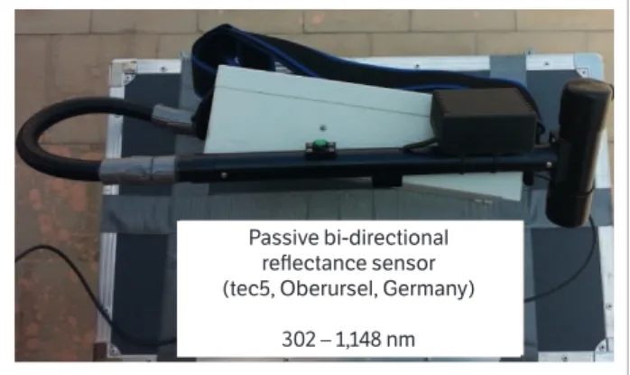
Description of passive sensor and spectral reflectance measurements
A passive bi-directional reflectance sensor (tec5, Oberursel, Germany) measuring wavelengths between 302 and 1,148 nm (Figure 1), with a bandwidth of 2 nm and connected to a portable computer and geographical positioning system (GPS), was used. The handheld FieldSpec sensor consists of 2 units. One unit was linked with a diffuser and measured the light radiation as a reference signal. The second unit measured the canopy reflectance with a fiber optic (Mistele and Schmidhalter 2008; Elsayed et al. 2015b), with an aperture of 12° and a
field of view of 0.2 m2 from 1 m of height. The aperture
of an optical system is the opening that determines the cone angle of a bundle of rays that enter the optics. The cone angle also depends on the optical material. The numerical aperture (α) is half of the cone angle, e.g. for fiber optics, it is 12°.
α is the apex angle or optical aperture [°]; A is the acquisition area.
The sensor outputs were co-recorded along with the GPS coordinates when collecting information in the field. The actual sensor output was co-referenced and recorded for each position. Afterwards, readings within 1 plot were averaged to a single value per plot. The canopy reflectance was calculated with the readings from the spectrometer unit and corrected with a calibration factor obtained from a reference grey standard. Spectral measurements were mostly taken on sunny days at nadir direction approximately 1.5 m above the canopy. Readings were taken once during main stem elongation (BBCH 39) at 08/03/2015 and ripening of fruits and seeds (BBCH 61) at 08/30/2014
Selection of spectral reflectance indices
In Table 1, 5 spectral indices from different sources are listed with the respective references. In this study, we calculated and tested both known and novel indices. A contour map analysis for all wavelengths of the hyperspectral passive sensor (from 302 to 1,048 nm) was used to select some normalised difference indices. The selected indices generally presented more stable and strong relationships with biomass fresh and dry weight, canopy water content, canopy water mass and grain yield of maize cultivars. All possible dual wavelength combinations were evaluated depending on a contour map analysis for the hyperspectral passive sensor. Contour maps are matrices of the coefficients of determination of all variable measurements with all possible combinations of binary, normalised spectral indices (Figure 2). The ‘lattice’ package from the software R statistics version 3.0.2 (R foundation for statistical computing 2013) was used to produce the contour maps from the hyperspectral reflectance readings; 7 wavelengths (720; 790; 880; 900; 940; 960; and 970 nm) were therefore used to calculate the reflectance indices given in Table 1.
r [m] = h * tan(α) (1) ;
A [m²] = π * r² (2) ;
where: r is the radius; h is the measuring height [m];
spectral reflectance indices Formula references
Normalised water index 1 (NWI-1) (R970 − R900)/(R970 + R900) Prasad et al. (2006)
Normalised water index 3 (NWI-3) (R970 − R880)/(R970 + R880) Babar et al. (2006)
Normalised water index 4 (NWI-4) (R970 − R900)/(R970 + R900) Gutierrez et al. (2010)
Normalised index based on 960 and 940 nm (R960 − R940)/(R960 + R940) Elsayed et al. (2011)
Normalised index based on 790 and 720 nm (R790 − R720)/(R790 + R720) Winterhalter et al. (2011)
table 1. Description of the spectral reflectance indices examined in this study.
Figure 1. A passive bi-directional reflectance sensor measuring wavelengths between 302 and 1,148 nm.
Passive bi-directional reflectance sensor (tec5, Oberursel, Germany)
Modelling of measured plant traits
Sigmaplot for Windows v.12 (Systat soft ware Inc, Chicago) and SPSS 22 (SPSS Inc, Chicago, IL, USA) were used for the statistical analysis. Simple linear regressions were calculated
to analyse the relationships between spectral indices listed in
Table 1 with the measured plant traits (Tables 2,3). Coeffi cients
of determination and signifi cance levels were determined; nominal alpha values and 0.001 were used (Table 4). In Table 5 and Figure 3 validation approach using fully independent data was used. Models were calibrated using
datasets of spectral index (R970 − R900)/(R970 + R900) in 2013
and validated using data in 2014 to predicted the measured
parameters. Th e quality of the validation models is presented
through adjusted coeffi cients of determination and the slope
and intercept of the linear regressions between observed and predicted values measured parameters.
Biomass fresh weigh, biomass dry weight, canopy water content, and canopy water mass
Biomass sampling was performed 2 times, at BBCH 39 in 2013 and at BBCH 61 in 2014. To determine biomass fresh weight (BFW), 3 plants were removed from each plot
and weighed. Th ereaft er, samples were placed in an oven
(65 °C) until there was no change in the biomass dry weight
(BDW). Th e canopy water content percentage (CWC %) was
calculated as CWC = (BFW − BDW)/(BFW − BDW). In
addition, canopy water mass (CWM kg/m2) was calculated as
CWM = (BFW − BDW)/A, where A is the area of biomass harvest.
Grain yield
Five samples for each plot were harvested by hand. Total the cob and grain yield of 5 samples was weighed for each plot, samples were oven-dried to determine grain water content on a gravimetric basis and the yield was expressed
as t∙ha−1,normalised to a water content of 14%
w. Plot yields
were averaged for each cultivar in each fi eld trial.
resuLts And discussion
Variation in biomass, water status, and grain yield of maize cultivars under
5 treatment in 2 years
Mean values of the measured variables, i.e. biomass fresh and dry weight, canopy water content, canopy water mass, and grain yield of the 5 maize cultivars subjected to 5 treatments (FI, FIMS, FIHS, WSMS, and WSHS) are shown in Tables 2,3.
W
a
v
elength – 2 nm
W
a
v
elength – 2 nm
W
a
v
elength – 2 nm
W
a
v
elength – 2 nm
1000
800
400 600
1,000
800
400 600
1,000
800
400 600
1,000
800
400 600
0.8 0.7 0.6 0.5 0.4 0.3
0.1 0.0 0.2
0.7 0.6 0.5 0.4 0.3
0.1 0.0 0.2
0.8 0.7 0.6 0.5 0.4 0.3
0.1 0.0 0.2
0.7 0.6 0.5 0.4 0.3
0.1 0.0 0.2
400 600 800 1,000
400 600 800 1,000
400 600 800 1,000
400 600 800 1,000
Wavelength – 1 nm
a
b
c
d
Figure 2. Correlation matrices (contour maps) showing the coeffi cients of determination (R2) for all dual wavelength combinations
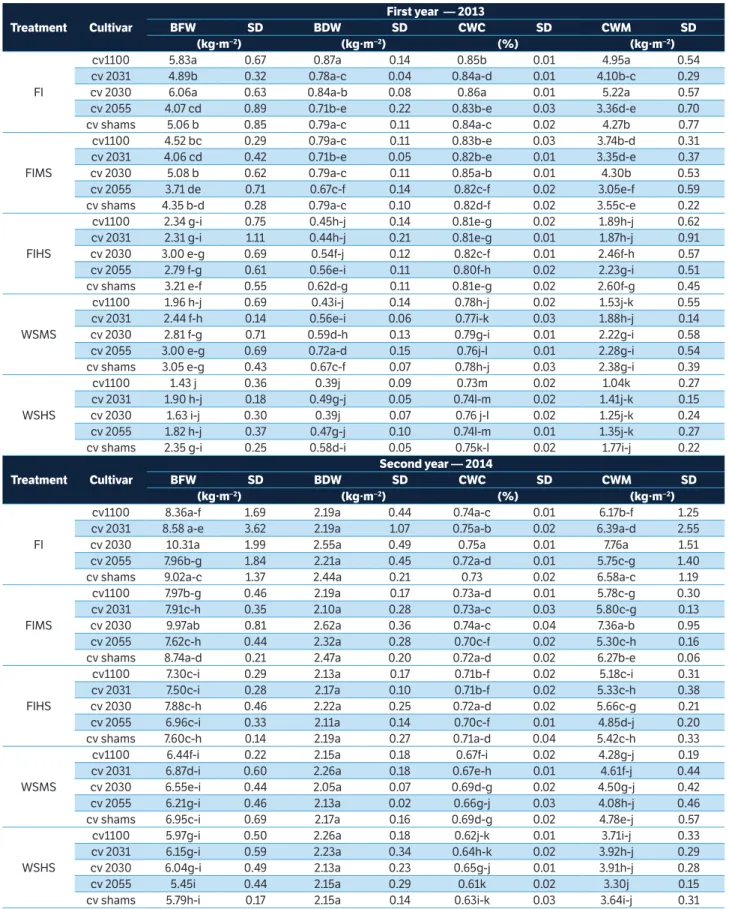
table 2. Average biomass fresh and dry weight, canopy water content, and canopy water mass of 5 maize cultivars under 5 treatments at 2 growth stages in 2013 and 2014. Values with the same letter are not significantly different (p ≥ 0.05) among treatments according to Duncan’s test.
treatment cultivar
First year — 2013
bFW sd bdW sd cWc sd cWM sd
(kg∙m−2) (kg∙m−2) (%) (kg∙m−2)
FI
cv1100 5.83a 0.67 0.87a 0.14 0.85b 0.01 4.95a 0.54
cv 2031 4.89b 0.32 0.78a-c 0.04 0.84a-d 0.01 4.10b-c 0.29
cv 2030 6.06a 0.63 0.84a-b 0.08 0.86a 0.01 5.22a 0.57
cv 2055 4.07 cd 0.89 0.71b-e 0.22 0.83b-e 0.03 3.36d-e 0.70
cv shams 5.06 b 0.85 0.79a-c 0.11 0.84a-c 0.02 4.27b 0.77
FIMS
cv1100 4.52 bc 0.29 0.79a-c 0.11 0.83b-e 0.03 3.74b-d 0.31
cv 2031 4.06 cd 0.42 0.71b-e 0.05 0.82b-e 0.01 3.35d-e 0.37
cv 2030 5.08 b 0.62 0.79a-c 0.11 0.85a-b 0.01 4.30b 0.53
cv 2055 3.71 de 0.71 0.67c-f 0.14 0.82c-f 0.02 3.05e-f 0.59
cv shams 4.35 b-d 0.28 0.79a-c 0.10 0.82d-f 0.02 3.55c-e 0.22
FIHS
cv1100 2.34 g-i 0.75 0.45h-j 0.14 0.81e-g 0.02 1.89h-j 0.62
cv 2031 2.31 g-i 1.11 0.44h-j 0.21 0.81e-g 0.01 1.87h-j 0.91
cv 2030 3.00 e-g 0.69 0.54f-j 0.12 0.82c-f 0.01 2.46f-h 0.57
cv 2055 2.79 f-g 0.61 0.56e-i 0.11 0.80f-h 0.02 2.23g-i 0.51
cv shams 3.21 e-f 0.55 0.62d-g 0.11 0.81e-g 0.02 2.60f-g 0.45
WSMS
cv1100 1.96 h-j 0.69 0.43i-j 0.14 0.78h-j 0.02 1.53j-k 0.55
cv 2031 2.44 f-h 0.14 0.56e-i 0.06 0.77i-k 0.03 1.88h-j 0.14
cv 2030 2.81 f-g 0.71 0.59d-h 0.13 0.79g-i 0.01 2.22g-i 0.58
cv 2055 3.00 e-g 0.69 0.72a-d 0.15 0.76j-l 0.01 2.28g-i 0.54
cv shams 3.05 e-g 0.43 0.67c-f 0.07 0.78h-j 0.03 2.38g-i 0.39
WSHS
cv1100 1.43 j 0.36 0.39j 0.09 0.73m 0.02 1.04k 0.27
cv 2031 1.90 h-j 0.18 0.49g-j 0.05 0.74l-m 0.02 1.41j-k 0.15
cv 2030 1.63 i-j 0.30 0.39j 0.07 0.76 j-l 0.02 1.25j-k 0.24
cv 2055 1.82 h-j 0.37 0.47g-j 0.10 0.74l-m 0.01 1.35j-k 0.27
cv shams 2.35 g-i 0.25 0.58d-i 0.05 0.75k-l 0.02 1.77i-j 0.22
treatment cultivar
second year — 2014
bFW sd bdW sd cWc sd cWM sd
(kg∙m−2) (kg∙m−2) (%) (kg∙m−2)
FI
cv1100 8.36a-f 1.69 2.19a 0.44 0.74a-c 0.01 6.17b-f 1.25
cv 2031 8.58 a-e 3.62 2.19a 1.07 0.75a-b 0.02 6.39a-d 2.55
cv 2030 10.31a 1.99 2.55a 0.49 0.75a 0.01 7.76a 1.51
cv 2055 7.96b-g 1.84 2.21a 0.45 0.72a-d 0.01 5.75c-g 1.40
cv shams 9.02a-c 1.37 2.44a 0.21 0.73 0.02 6.58a-c 1.19
FIMS
cv1100 7.97b-g 0.46 2.19a 0.17 0.73a-d 0.01 5.78c-g 0.30
cv 2031 7.91c-h 0.35 2.10a 0.28 0.73a-c 0.03 5.80c-g 0.13
cv 2030 9.97ab 0.81 2.62a 0.36 0.74a-c 0.04 7.36a-b 0.95
cv 2055 7.62c-h 0.44 2.32a 0.28 0.70c-f 0.02 5.30c-h 0.16
cv shams 8.74a-d 0.21 2.47a 0.20 0.72a-d 0.02 6.27b-e 0.06
FIHS
cv1100 7.30c-i 0.29 2.13a 0.17 0.71b-f 0.02 5.18c-i 0.31
cv 2031 7.50c-i 0.28 2.17a 0.10 0.71b-f 0.02 5.33c-h 0.38
cv 2030 7.88c-h 0.46 2.22a 0.25 0.72a-d 0.02 5.66c-g 0.21
cv 2055 6.96c-i 0.33 2.11a 0.14 0.70c-f 0.01 4.85d-j 0.20
cv shams 7.60c-h 0.14 2.19a 0.27 0.71a-d 0.04 5.42c-h 0.33
WSMS
cv1100 6.44f-i 0.22 2.15a 0.18 0.67f-i 0.02 4.28g-j 0.19
cv 2031 6.87d-i 0.60 2.26a 0.18 0.67e-h 0.01 4.61f-j 0.44
cv 2030 6.55e-i 0.44 2.05a 0.07 0.69d-g 0.02 4.50g-j 0.42
cv 2055 6.21g-i 0.46 2.13a 0.02 0.66g-j 0.03 4.08h-j 0.46
cv shams 6.95c-i 0.69 2.17a 0.16 0.69d-g 0.02 4.78e-j 0.57
WSHS
cv1100 5.97g-i 0.50 2.26a 0.18 0.62j-k 0.01 3.71i-j 0.33
cv 2031 6.15g-i 0.59 2.23a 0.34 0.64h-k 0.02 3.92h-j 0.29
cv 2030 6.04g-i 0.49 2.13a 0.23 0.65g-j 0.01 3.91h-j 0.28
cv 2055 5.45i 0.44 2.15a 0.29 0.61k 0.02 3.30j 0.15
cv shams 5.79h-i 0.17 2.15a 0.14 0.63i-k 0.03 3.64i-j 0.31
.
BFW = Biomass fresh weight; SD = Standard deviation; BDW = Biomass dry weight; CWC = Canopy water content; CWM = Canopy water mass; FI = Full irrigation without salinity; FIMS = Full irrigation with medium salinity level, 3 dS∙m−1; FIHS = Full irrigation with high salinity level, 5 dS∙m−1; WSMS = Water stress with medium
treatment cultivar
First year — 2013 second year — 2014
cY sd gY sd cY sd gY sd
(t∙ha−1)
FI
cv1100 13.3a 1.37 8.9a 1.06 12.4 a-c 0.57 8.1a-b 0.86
cv 2031 11.3a-h 1.29 6.7b-h 0.83 10.7a-j 0.29 6.3b-j 0.57
cv 2030 12.6ab 1.29 7.2a-f 0.84 12.0a-d 0.29 6.9a-g 0.29
cv 2055 10.8a-j 3.87 6.6b-h 2.31 10.3a-k 1.14 6.3b-i 0.92
cv shams 12.3a-c 1.94 7.7a-e 1.11 11.5a-g 0.88 7.9a-c 0.34
FIMS
cv1100 11.4a-g 2.75 6.3b-j 1.52 8.7c-m 2.57 5.1f-m 1.10
cv 2031 10.6a-j 2.26 6.2b-k 1.17 8.7c-m 1.61 5.5e-m 0.85
cv 2030 11.9a-e 2.85 6.9a-g 1.50 9.0b-m 1.51 6.0b-l 0.65
cv 2055 9.3b-m 1.08 5.0f-m 1.61 9.2b-m 2.46 5.8c-m 1.38
cv shams 11.9a-c 0.74 7.8a-d 0.64 9.6a-m 2.48 5.5e-m 1.52
FIHS
cv1100 10.1a-l 0.82 5.6d-m 0.47 7.5h-n 1.61 4.3i-n 1.39
cv 2031 10.1a-l 1.48 6.0b-l 1.15 7.9g-n 2.55 4.6h-n 1.39
cv 2030 11.2a-f 2.05 7.0a-g 1.32 9.0b-m 2.44 6.1b-l 1.06
cv 2055 9.0b-m 1.92 6.1b-k 1.27 7.5i-n 2.58 5.0g-m 1.35
cv shams 10.7a-f 1.70 6.9a-g 1.08 8.1e-m 1.73 4.8g-n 1.23
WSMS
cv1100 8.2d-m 2.43 4.8g-n 1.63 7.2j-n 1.15 3.9k-n 0.83
cv 2031 9.1b-m 2.39 4.8g-n 1.24 6.4l-n 1.61 3.7m-n 0.81
cv 2030 10.7a-j 1.09 6.8a-g 0.74 7.3j-n 1.90 4.3i-n 1.24
cv 2055 9.2b-m 1.47 5.7d-m 1.20 6.8g-n 1.87 5.2f-m 1.26
cv shams 10.2a-i 3.01 6.4b-i 1.42 7.5h-n 0.32 4.4i-n 0.19
WSHS
cv1100 7.8g-n 1.02 4.4h-n 0.69 6.3m-n 1.79 4.0j-n 0.85
cv 2031 8.0f-m 3.93 4.9g-n 1.94 4.4n 0.49 2.7m 0.14
cv 2030 9.7a-m 1.70 6.2b-j 0.99 6.8k-n 1.22 4.4i-n 0.92
cv 2055 8.9b-m 1.70 5.7d-m 1.29 6.5l-n 1.58 3.9l-n 1.03
cv shams 8.5d-m 1.15 5.4f-m 0.91 6.4l-n 1.47 3.6m-n 1.04
table 3. Average cob and grain yield of 5 maize cultivars under 5 treatments at 2 growth stages in 2013 and 2014. Values with the same letter are not significantly different (p ≥ 0.05) among treatments according to Duncan’s test.
CY = Cob yield; SD = Standard deviation; GY = Grain yield; FI = Full irrigation without salinity; FIMS = Full irrigation with medium salinity level, 3 dS∙m−1; FIHS = Full
irrigation with high salinity level, 5 dS∙m−1; WSMS = Water stress with medium salinity level; WSHS = Water stress with high salinity level.
Year and growth
stage parameters
(r790 − r720) / (r790 + r720)
(r960 − r940)/ (r960 + r940)
(r970 − r880)/ (r970 + r880)
(r970 − r900)/ (r970 + r900)
(r970 − r920)/ (r970 + r920)
2013 CWC 0.68*** 0.61*** 0.69*** 0.70*** 0.69***
BBCH 39 CWM 0.65*** 0.65*** 0.63*** 0.66*** 0.67***
DW 0.49*** 0.56*** 0.51*** 0.56*** 0.57***
FW 0.64*** 0.65*** 0.62*** 0.66*** 0.67***
CY 0.72*** 0.73*** 0.69*** 0.73*** 0.75***
GY 0.48*** 0.51*** 0.52*** 0.52*** 0.52***
2014 CWC 0.00 0.14 0.63*** 0.65*** 0.61***
BBCH 61 CWM 0.06 0.23* 0.68*** 0.72*** 0.70***
DW 0.24* 0.21* 0.26** 0.29** 0.29**
FW 0.08 0.25** 0.67*** 0.71*** 0.69***
CY 0.12 0.27** 0.59*** 0.66*** 0.66***
GY 0.09 0.20* 0.57*** 0.61*** 0.61***
table 4. Coefficients of determination of linear regressions of 6 measured parameters with spectral indices of the hyperspectral passive sensor (calculated as normalised difference indices) for maize cultivars subjected to 5 treatments in 2013 and 2014.
*,**,***Statistically significant at p ≤ 0.05, p ≤ 0.01, and p ≤ 0.001, respectively. CWC = Canopy water content; CWM = Canopy water mass; DW = Dry weight;
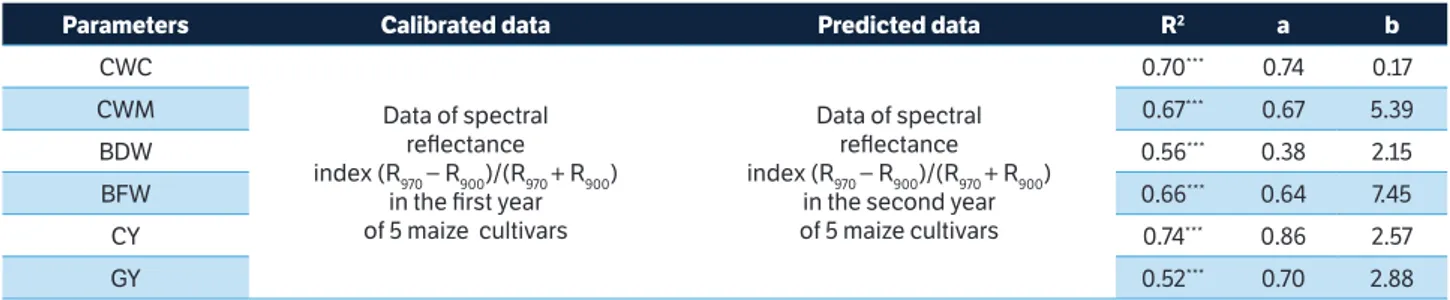
parameters calibrated data predicted data r2 a b
CWC
Data of spectral reflectance index (R970 − R900)/(R970 + R900)
in the first year of 5 maize cultivars
Data of spectral reflectance index (R970 − R900)/(R970 + R900)
in the second year of 5 maize cultivars
0.70*** 0.74 0.17
CWM 0.67*** 0.67 5.39
BDW 0.56*** 0.38 2.15
BFW 0.66*** 0.64 7.45
CY 0.74*** 0.86 2.57
GY 0.52*** 0.70 2.88
table 5. Models of spectral reflectance index (R970 − R900)/(R970 + R900) of the hyperspectral passive reflectance sensor.
***Statistically significant at p ≤ 0.001. CWC, CWM, BDW, BFW, CY, GY were calibrated depending on spectral data of first year of 5 maize cultivars. Calibration
functions were validated with independent data measured on the indicated prediction data. Coefficients of determination (R2), slopes (a), and intercepts (b) of these linear validation functions between observed and predicted values of all parameters are shown. CWC = Canopy water content; CWM = Canopy water mass; BDW = Biomass dry weight; BFW = Biomass fresh weight; CY = Cob yield; GY = Grain yield.
Generally, the highest mean values of all variables were recorded under irrigation without salt of all cultivars for each year, and the lowest values for the measured variables were recorded at high salinity level with water
Figure 3. Relationship between the spectral index (R970 – R900)/(R970 + R900) with canopy water content (CWC), canopy water mass (CWM), biomass fresh weight (BFW), biomass dry weight (BDW), cob yield (CY), and grain yield (GY) of maize cultivars under 5 treatments in 2014.
R2 = 0.70***
R2 = 0.56***
R2 = 0.73***
R2 = 0.66***
R2 = 0.66***
R2 = 0.52***
CWC (%) CWM (kg∙m–2)
BFW (kg∙m–2)
0.70 0.72 0.74 0.76 0.78 0.80 0.82 0.84 0.86 0.88 -0.055 -0.050 -0.045 -0.040 -0.035 -0.030 -0.025 -0.020 -0.015 (R 97 0 – R 900 )/(R 97 0 + R 900 ) (R 97 0 – R 900 )/(R 97 0 + R 900 ) (R 97 0 – R 900 )/(R 97 0 + R 900 ) (R 97 0 – R 900 )/(R 97 0 + R 900 ) (R 97 0 – R 900 )/(R 97 0 + R 900 ) (R 97 0 – R 900 )/(R 97 0 + R 900 )
0 1 2 3 4 5 6
-0.055 -0.050 -0.045 -0.040 -0.035 -0.030 -0.025 -0.020 -0.015
BDW (kg∙m–2)
0.3 0.4 0.5 0.6 0.7 0.8 0.9
-0.055 -0.050 -0.045 -0.040 -0.035 -0.030 -0.025 -0.020 -0.015
1 2 3 4 5 6 7
-0.055 -0.050 -0.045 -0.040 -0.035 -0.030 -0.025 -0.020 -0.015
CY (t∙ha–1) GY (t∙ha–1)
8 10 12 14
-0.055 -0.050 -0.045 -0.040 -0.035 -0.030 -0.025 -0.020 -0.015
4 5 6 7 8 9 10
-0.055 -0.050 -0.045 -0.040 -0.035 -0.030 -0.025 -0.020 -0.015
stress. There was a clear difference between treatments of the 5 maize cultivars for each year. The mean values
for first year ranged from 1.43 to 6.06 kg∙m−2 for biomass
weight, from 0.73 to 0.86% for canopy water mass, from
1.04 to 4.95 kg∙m−2 for canopy water mass, from 7.8 to
13.3 t∙ha−1 for cob yield and from 4.4 to 8.9 t∙ha−1 for grain
yield. Generally, full irrigation with salinity levels and the interaction between full irrigation with high salinity level and water stress in 2 years tended to decrease all measured parameters. The measured parameters were affected by the treatments at filling growth stage in 2014 than at vegetation growth stage in 2013. These results agree
with other reports (Dooronbos and Kassam 1979)which
found that great grain yield reduction is caused by water deficit during flowering period and maize is moderately sensitive to salinity. The grain yield of maize gradually was decreased by increasing salinity levels of soil. It was decreased by 10; 25; 50; and 100% at 2.5; 3.8; 5.9; and
10 dS∙m−1, respectively. In the same way, salt stress in maize,
during the reproductive phase, decreases grain weight and the number of grains per cob (Abdullah et al. 2001; Kaya et al. 2013). Azevedo Neto et al. (2005) concluded
that salinity (25 mmol∙L−1 per day NaCl salt for 15 days)
reduced the dry mass of maize shoot and root. The shoot dry weight reduced from 33.8 to 66.5% while root dry weight decreased by up to 61.4%. The different genotypes
response was due to their variable tolerance.Dordipour
(2004) reported that the effect of salinity depends on the stage at which the plant is exposed to this stress. The cv 2030 and cv shams cultivars are more tolerant to salinity and water stress.
Contour map analysis of the hyperspectral passive data
A contour map analysis produced the mean coefficients
of determination (R2) of the 2 measurement dates in
2013 and 2014 for all dual wavelength combinations as a normalised difference spectral index. The contours of the matrices of the hyperspectral passive sensor presented more distinct relationships between measure plant parameters, such biomass fresh and dry weight, canopy water content, canopy water mass, and grain yield of the 5 maize cultivars subjected to 5 treatments in the near infrared wavelengths than with the visible wavelengths. The contour map analysis of the relationship between the normalised difference spectral indices with canopy water content and biomass fresh weight in 2013 as well as with cob and grain yield in 2014 are shown in Figure 2.
These results agree with other reports (Elsayed et al.
2015b) which found that the wavelengths at area of near infrared is more distinct related to the grain yield and normalised relative canopy temperature of barley cultivars under water stress conditions.
The relationship between spectral
reflectance indices with different measured plant parameters
Across the 2 measuring times, 5 spectral indices were more closely correlated with biomass fresh and dry weight, canopy water content, canopy water mass, and grain yield of the 5 maize cultivars subjected to 5 treatments. The obtained coefficients of determination
(R2) are shown in Table 4 and Figure 3. Statistically
significant relationships between all spectral reflectance indices derived from near infrared (NIR) were found
for BFW (R2 values ranging from 0.25** to 0.72***),
BDW (R2 values ranging from 0.21* to 0.57***), CWC
(R2 values ranging from 0.61*** to 0.70***), CWM (R2 values
ranging from 0.23** to 0.72***), CY (R2 values ranging
from 0.27*** to 0.75***), and GY (R2 values ranging from
0.20* to 0.61***) are shown in Table 4. Generally, the
normalised water indices of (R970 − R900)/(R970 + R900)
and (R970 − R880)/(R970 + R880) and (R970 − R920)/(R970 + R920) showed the highest coefficients of determination for the measured variables in the 2 years. These results are in agreement with Lobos et al. (2014), who found that the
normalised water index NWI-3: (R970 − R920)/(R970 + R920)
and the normalised difference vegetation index NDVI:
(R830 − R660)/(R830 + R660) indicated closer relationships
(R2 values of 0.66 and 0.62) with the GY of wheat cultivars
under mild drought stress compared with severe drought
stress (R2 values of 0.58 and 0.40). Additionally, Gutierrez
et al. (2010) and Elsayed et al. (2015b) found that the
normalised water indices NWI-1: (R970 − R900)/(R970 + R900)
and NWI-3: (R970 − R920)/(R970 + R920) of a hyperspectral
passive sensor presented significant relationships with the grain yield of wheat genotypes and barley cultivars under drought stress. As well as the spectral index
(R790 − R720)/(R790 + R720) correlated to the biomass and
There were significant relationships between the observed and predicted of all parameters. The slopes of the vali- dation regression lines were generally less than 1. In the independent validation in Table 5, the highest coefficient
of determination was R2 = 0.74, and the highest slope
recorded was 0.86 for CY. The validation models seem to be good to predicted CY, GY, and CWC. The validation models are more difficult to predict CWM, BFW, and BDW. Maybe, this is due to the effect of the growth stage and year in spectral reflectance. These results agree with the findings by Elsayed et al. (2011), who reported that the spectral reflectance was influenced by the growth stage of the plant.
concLusion
From the mentioned results, it can be concluded that the 3 water indices seem to be good indicators to detect the water status, biomass, and yield of maize cultivars under irrigation and under interaction between salinity and water stress treatments. The model developed from the water spectral index analysis reliably assessed the CWC, CY and GY. The measured parameters were more affected by the treatment (full irrigation with high salinity level and water stress) compared to other treatments.
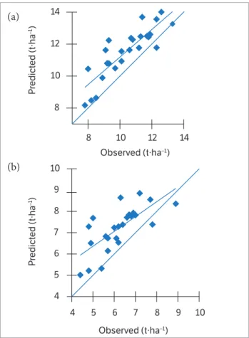
Figure 4. Scatter plots and linear regressions between observed and predicted values of (a) cob yield, (b) grain yield, and their predicted values from dataset of spectral reflectance index (R970 − R900)/(R970 + R900). Statistical information is given in Table 5.
Observed (t∙ha–1)
8 10 12 14
P
redict
ed (t∙ha
–1)
P
redict
ed (t∙ha
–1)
8 10 12 14
Observed (t∙ha–1)
4 5 6 7 8 9 10
4 5 6 7 8 9 10
Abdullah Z., Khan M.A. and Flowers T.J. (2001). Causes of sterility in seed
set of rice under salinity stress. Journal of Agronomy and Crop Science,
187, 25-32. http://dx.doi.org/10.1046/j.1439-037X.2001.00500.x.
Abu-Zied, M. (1999). Egypt’s Water Policy for the 21st Century.
Proceedings of the 7th Nile Conference; Cairo, Egypt.
Allen, R. G., Pereira, L. S., Raes, D. and Smith, M. (1998). Crop
evapotranspiration. Guidelines for computing crop water
requirements. FAO Irrigation and Drainage. Paper No. 56. Rome: FAO.
Azevedo Neto, A. D, Prisco, J. T., Enéas-Filho, J., Medeiros, J. R. and
Gomes Filho, E. (2005). Hydrogen peroxide pre-treatment induces
salt stress acclimation in maize plants. Journal of Plant Physiology,
162, 1114-1122. http://dx.doi.org/10.1016/j.jplph.2005.01.007.
Babar, M. A., van Ginkel, M., Klatt, A. R., Prasad, B. and Reynolds,
M. P. (2006). The potential of using spectral reflectance indices to
reFerences
estimate yield in wheat grown under reduced irrigation. Euphytica,
150, 155-172.
Carter, G. A. (1991). Primary and secondary effects of water content
on the spectral reflectance of leaves. American Journal of Botany,
78, 916-924. http://dx.doi.org/10.2307/2445170.
Dooronbos, J. and Kassam, A. H. (1979). Yield response to water.
FAO Irrigation and Drainage, Paper no. 33. Rome: FAO.
Dordipour, I. (2004). Use of Caspian sea water for irrigiation (PhD
thesis). Tehran: Tarbiat Modarres University. In Persian.
El-Hendawy, S., Al-Suhaibani, N., Salem, A., Ur Rehman, S. and Schmidhalter,
U. (2015). Spectral reflectance indices as a rapid nondestructive
phenotyping tool for estimating different morphophysiological traits of
contrasting spring wheat germplasms under arid conditions. Turkish
Journal of Agriculture and Forestry, 39, 572-587.
(a)
Elsayed, S., Elhoweity, M. and Schmidhalter, U. (2015a). Normalized
difference spectral indices and partial least squares regression
to assess the yield and yield components of peanut. Australian
Journal of Crop Science, 9, 976-986.
Elsayed, S., Mistele, B. and Schmidhalter, U. (2011). Can changes
in leaf water potential be assessed spectrally? Functional Plant
Biology, 38, 523-533.
Elsayed, S., Rischbeck, P. and Schmidhalter, U. (2015b). Comparing
the performance of active and passive reflectance sensors to assess the
normalized relative canopy temperature and grain yield of
drought-stressed barley cultivars. Field Crop Research, 177, 148-160.
Gutierrez, M., Reynolds, M. P., Raun, W. R., Stone, M. L. and Klatt,
A. R. (2010). Spectral water indices for assessing yield in elite
bread wheat genotypes in well irrigated, water stressed, and high
temperature conditions. Crop Science, 50, 197-214.
Hackl, H., Mistele, B., Hu, Y. and Schmidhalter, U. (2013).Spectral
assessments of wheat plants grown in pots and containers under
saline conditions. Functional Plant Biology, 40, 409-424.
Kaya, C., Ashraf, M., Dikilitas, M. and Tuna, A. L. (2013). Alleviation of
salt stress induced adverse effects on maize plants by exogenous
application of indoleacetic acid (IAA) and inorganic nutrients-a
field trial. Australian Journal of Crop Science, 7, 249-254.
Kipp, S., Mistele, B. and Schmidhalter, U. (2014). The performance
of active spectral reflectance sensors as influenced by measuring
distance, device temperature and light intensity. Computers and
Electronics in Agriculture, 100, 24-33.
Lobos, G.A., Matus, I., Rodriguez, A., Romero-Bravo, S., Araus,
J. L. and Pozo, A. D. (2014). Wheat genotypic variability in grain
yield and carbon isotope discrimination under Mediterranean
conditions assessed by spectral reflectance. Journal of
Integrative Plant Biology, 56, 470-479. http://dx.doi.org/10.1111/
jipb.12114.
Marti, J., Bort, J., Slafer, G. A. and Araus, J. L. (2007). Can wheat
yield be assessed by early measurements of normalized difference
vegetation index? Annals of Applied Biology, 150, 253-257.
Mistele, B. and Schmidhalter, U. (2008). Estimating the nitrogen
nutrition index using spectral canopy reflectance measurements.
European Journal of Agronomy, 29, 184-190.
Peñuelas, J., Filella, I. and Serrano, L. (1993). The reflectance at the
950–970 nm region as an indicator of plant water status. International
Journal of Remote Sensing, 14, 1887-1905.
Prasad, B., Carver, B. F., Stone, M. L., Babar, M. A., Raun, W. R. and
Klatt, A.R. (2006). Potential use of spectral reflectance indices as
a selection tool for grain yield in winter wheat under Great Plains
conditions. Crop Science, 47, 1426-1440. http://dx.doi.org/10.2135/
cropsci2006.07.0492.
Schmidhalter, U. (2005). Development of a quick on-farm test to
determine nitrate levels in soil. Journal of Plant Nutrition and Soil
Science, 168, 432-438.
Thoren, D. and Schmidhalter, U. (2009). Nitrogen status and
biomass determination of oilseed rape by laser-induced chlorophyll
fluorescence. European Journal of Agronomy, 30, 238-242.
Winterhalter, L., Mistele, B., Jampatong, S. and Schmidhalter,
U. (2011). High throughput phenotyping of canopy water mass
and canopy temperature in well-watered and drought stressed
tropical maize hybrids in the vegetative stage. European Journal of
Agronomy, 35, 22-32. http://dx.doi.org/10.1016/j.eja.2011.03.004.
Winterhalter, L., Mistele, B. and Schmidhalter, U. (2013). Evaluation
of active and passive sensor systems in the field to phenotype maize
hybrids with high-throughput. Field Crops Research, 154, 236-245.
Woolley, J. T. (1971). Reflectance and transmittance of light by
leaves. Plant Physiology, 47, 656- 662.
Wu, C., Niu, Z., Tang, Q. and Huang, W. (2009). Predicting vegetation
water content in wheat using normalized difference water indices
derived from ground measurements. Journal of Plant Research, 122,
317- 326. http://dx.doi.org/10.1007/s10265-009-0215-y.
Yonghong, Y.I., Yang, D., Chen, D. and Hung, J. (2007). Retrieving
crop physiological parameters and assessing deficiency using
MODIS data during the winter wheat growing period. Canadian