PEDRO DEYRIEUX CENTENO OGANDO
DOS SANTOS
Licenciado em Engenharia do Ambiente
Heavy metals removal in dual media
filters
Orientador: Prof. Doutora Leonor Amaral, FCT/UNL Co ‑orientador: Eng.ª Diana Brandão, TU Delft
Outubro 2012
Dissertação para obtenção do Grau de Mestre em Engenharia do Ambiente – Perfil de Engenharia Sanitária
Júri:
Heavy metals removal in dual media filters
© Copyright em nome de Pedro Deyrieux Centeno Ogando dos Santos, FCT/UNL
«You can’t build a reputation on what you are going to do…» Henry Ford (1863 ‑1947)
ACKNOWLEDGEMENTS
The research project that supports this thesis was carried out at the Water Management Depart‑ ment of Civil Engineering Faculty (CiTG) at Delft University of Technology (TU Delft), from February until July 2011.
Thanks to TU Delft, it was possible to perform the practical work in Harnaschpolder’s wastewater treatment plant (WWTP), one of the biggest in Europe. During the research I was able to learn not only from the university staff but also from the people at the plant and/or companies I had to work with, when this project was developed.
I would like to express my gratitude to Leonor Amaral, my supervisor in Lisbon and to Diana Brandão, my supervisor in Delft, for all the support and their availability.
I also would like to express my appreciation to everyone in the Sanitary Department of TU Delft for their friendship and daily support, especially to Soledad Villarroel, Tony Schuit, Patrick Andeweg, Mieke Hubert and also the people at the plant (Sigrid Scherrenberg, Han van de Griek and others).
RESUMO
O presente estudo pretendeu investigar mecanismos de remoção físico ‑químicos de metais pesados (nomeadamente de precipitação) de águas residuais tratadas da ETAR de Harnaschpolder, localizada no Sul da Holanda, para que seja possível a produção de dois tipos de águas de qualidade diferentes: águas «superficiais» e águas para a irrigação em estufas.
Para tal, foram construídos dois filtros de dupla camada na estação piloto da ETAR de Harnas‑ chpolder. Após montagem e operação inicial dos filtros, concentrações específicas de metais pesados (Cd, Cu, Ni e Zn) foram doseadas a montante do processo, e estudou‑se a remoção dos metais pesa‑ dos. Num projecto paralelo a este, foi também estudada a remoção destes metais pesados através da inoculação de bactérias específicas.
Curvas de solubilidade foram construídas, utilizando o software PHREEQc, para simular as con‑ dições existentes nos filtros (pH, temperatura, alcalinidade, etc.) e calcular a probabilidade de precipi‑ tação dos metais pesados quando sujeitos as estas condições, de forma a confirmar a remoção (ou a não remoção) destes metais.
Os resultados tanto das experiências como da simulação sugerem que a precipitação de metais pesados (sobre a forma de hidróxidos, carbonetos e carbonatos, cianetos, sulfatos e sulfitos) não tenha ocorrido, devido às condições inerentes dos filtros. Os resultados sugerem ainda que outros mecanismos estejam envolvidos na remoção destes metais, possivelmente adsorção e/ou quelação.
ABSTRACT
The purpose of this study was to investigate physicochemical mechanisms for the removal of heavy metals from the effluent of Harnaschpolder’s WWTP Pilot Installation in the South of Netherlands. This effluent is partially submitted to tertiary treatment in a water reuse pilot which aims the production of water for two different end ‑uses: crop irrigation in greenhouses and surface ‑type water.
Tertiary filters were mounted and started up at the reuse pilot and specific concentrations of heavy metals were dosed in the filters. Removal efficiencies were then calculated after the end of the experi‑ ments. As a parallel research project, the removal of HM was also carried out by inoculating selected bacteria (biosorption).
Solubility curves were calculated for the dosed heavy metals (Cd, Cu, Ni, Zn) using PHREEQc programme, to predict if heavy metal precipitation occurred in the filters (using the same experimental data: temperature, pH , alkalinity, etc.).
Results show that physicochemical precipitation was not the primary removal mechanism for heavy metals. The results suggest that other mechanisms such as adsorption and/or chelation may be involved in the removal of these species.
LIST OF ABBREVIATIONS AND SYMBOLS
Cd – Cadmium
CdCO3 – Cadmium carbonate
Cd(OH)2 – Cadmium hydroxide
cmWC – centimeters of Water Column
Cr – Cromium
Cu – Copper
CuCO3– Copper carbonate
Cu(OH)2– Copper hydroxide
COD – Chemical Oxygen Demand
CSF – Continuous Sand Filtration
DMF – Dual Media Filter
FFFM (or 3FM) – Flexible Fiber Filter Module
Hg – Mercury
HM – Heavy Metal(s)
HNP – Harnaschpolder
HRT – Hydraulic Retention Time
ICP ‑MS – Inductively Coupled Plasma – Mass Spectrometry
MeOH – Methanol
MERESAFIN – MEtal REmoval by SAnd Filtration INoculation
MF – Micro Filtration
MMSF – Multi Media Sand Filtration
MS – Mother Solution (of heavy metals)
MTR – Maximum Tolerable Risk
NF – Nanofiltration
Ni – Nickel
Ni(OH)2– Nickel hydroxide
NO3 – Nitrate
NTU – Nephelometric Turbidity Units
NW4 – «Notavierde Water 4»: Fourth National Policy Document on Water Management
Pb – Lead
PHREEQc – Computer Program for Speciation, Batch ‑Reaction, One ‑Dimensional Transport, and Inverse Geochemical Calculations
RO – Reverse Osmosis
RPM – Revolutions Per Minute
SBBR – Static Bed Bio ‑Reactor
SWL – Supernatant Water Level
Tr – Filter run time
TSS – Total Suspended Solids
UF – Ultra Filtration
VRO – Vertical Reverse Osmosis
WWTP – Wastewater Treatment Plant
Zn – Zinc
Zn(CO3) – zinc carbonate or «smithsonite»
Zn(CO3).H2O – zinc carbonate monohydrated
TABLE OF CONTENTS
1. INTRODUCTION. . . 3
1.1 General Overview . . . 3
1.2 Quality standards for surface water – Heavy Metals. . . 4
1.3 The Harnaschpolder WWTP. . . 6
1.4 Harnaschpolder’s (treated) wastewater parameters . . . 8
2. OBJECTIVES OF THE RESEARCH. . . 9
3. OVERVIEW OF THE RESEARCH . . . 11
4. LITERATURE REVIEW . . . 13
4.1 Heavy metal removal processes. . . 13
– Dual media filtration. . . 16
4.2 Heavy metal removal mechanisms . . . 17
– Hydroxide precipitation . . . 18
– Sulfite precipitation . . . 19
– Carbonate precipitation . . . 21
– Cyanide precipitation. . . 22
– Heavy metal chelating precipitation . . . 22
– Bio ‑precipitation . . . 23
– Chemical Adsorption. . . 23
– Denitrification and heavy metals removal . . . 24
4.3 PHREEQc Software Simulation. . . 25
– Software potential in water and wastewater treatment. . . 26
5. MATERIALS AND METHODS . . . 27
5.1 PHREEQc Simulation. . . 30
– Development of the input file . . . 30
– Writing the input file. . . 31
– The output file. . . 33
5.2 Filter operation. . . 34
– Filters set ‑up. . . 34
– First run of experiments – «start up» . . . 41
– Filters backwash. . . 42
– Heavy metals dosing and measurements. . . 44
– Filter operation . . . 45
6. RESULTS AND DISCUSSION . . . 48
6.1 Results obtained using PHREEQc software. . . 48
– Cadmium equilibrium diagram . . . 48
– Copper equilibrium diagram. . . 50
– Nickel equilibrium diagram. . . 53
– Zinc equilibrium solubilities . . . 55
6.2 Removal of heavy metals in the filters. . . 58
– Pressure readings. . . 58
– Turbidity . . . 62
– Heavy metal removal. . . 65
7. CONCLUSIONS . . . 71
7.1 PHREEQc Simulation. . . 71
7.2 Filter Experiments . . . 71
8. FURTHER RESEARCH RECOMMENDATIONS . . . 73
8.1 PHREEQc Software Simulation. . . 73
8.2 Filter experiments. . . 73
LIST OF TABLES
Table 1. Maximum contaminant level of heavy metals in surface water and their toxicities to humans 4 Table 2. Maximum permissible risk (MTR) compared with average quality of the HNP’s WWTP 5
Table 3. Summary of the different possibilities of physicochemical removal for wastewater. . . 15
Table 4. Heavy metals removal by using chemical precipitation . . . 18
Table 5. Physicochemical parameters used in SOLUTION 1. . . 32
Table 6. PHREEQc output section. . . 33
Table 7. Dimensions and operational parameters of the lab‑scale filters. . . 37
Table 8. Summary of effects of independent variables on length of filter run . . . 42
Table 9. Heavy metals concentration for mother solution. . . 44
Table 10. Physicochemical parameters measured in the filters . . . 45
Table 11. Percentage of copper removal from filtration tests . . . 52
Table 12. Percentage of nickel removal from filtration tests . . . 55
LIST OF FIGURES
Figure 1. Treatment stages of the Harnaschpolder WWTP . . . 5
Figure 2. Schematics of the Water Reclamation Pilot in the Harnaschpolder WWTP. . . 6
Figure 3. Solubility of hydroxides and sulfides as a function of pH . . . 16
Figure 4. Zinc solubility diagram as function of pH . . . 23
Figure 5. Nickel solubility diagram as function of pH. . . 23
Figure 6. Copper solubility diagram as function of pH. . . 24
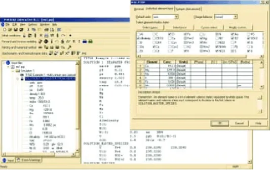
Figure 7. Main screen of PHREEQC, with the SOLUTION keyword dialog box open.. . . 26
Figure 8. Detail of the feeding system . . . 30
Figure 9. Dual media filters HNP’s Pilot Plant. . . 30
Figure 10. Detail of the filter column. . . 31
Figure 11. Schematics of the setup for the filtration experiments . . . 33
Figure 12. Effluent regulator box . . . 34
Figure 13. The backwash system in operation . . . 36
Figure 14. Concept design for filter experiments with selected pure bacteria . . . 41
Figure 15. Filters assembly at Harnaschpolder’s Pilot Plant . . . 42
Figure 16. Cadmium equilibrium diagram. . . 44
Figure 17. Copper equilibrium diagram . . . 46
Figure 18. Nickel equilibrium diagram . . . 48
Figure 19. Zinc equilibrium diagram. . . 51
Figure 20. Lindquist diagram for the dual media filter during filter run time for both filters A or B 54
Figure 21. Lindquist diagram for the filters A or B, during filter run time with addition of HM . . . . 55
Figure 22. Increase in head loss in filters with no addition of heavy metals (nor carbon). . . 56
Figure 23. Turbidity removal with no addition of heavy metals nor carbon (Filter A). . . 57
Figure 24. Turbidity removal with no addition of heavy metals nor carbon (Filter B) . . . 57
Figure 25. Turbidity removal with addition of HM for Filter A (no carbon) . . . 58
Figure 27. Dissolved HM removal with addition of HM – Filter A . . . 60
Figure 28. Dissolved HM removal with addition of HM – Filter B . . . 60
Figure 29. Total HM removal with addition of HM – Filter A . . . 61
APPENDIXES
Appendix I. Filter Design – First drawing . . . 64
Appendix II. Filter Design – Detailed Setup . . . 65
Appendix III. Filter Design – Detailed Setup (2) . . . 66
Appendix IV. Filter «start ‑up» manual. . . 67
Appendix V. Filter operation manual. . . 69
Appendix VI. Results of the filter experiments. . . 70
Appendix VII. Cadmium input file. . . 71
Appendix VIII. Copper input file. . . 72
Appendix IX. Nickel input file. . . 73
This thesis describes the work done by the author in the department of Water Management in the Civil Engineering and Geosciences building (CiTG), at the Technical University of Delft in the Nether‑ lands. It was supervised there by Diana Brandão in the scope of a project research on water reclamation, under the promotion of Professor ir. Jules van de Lier. This MSc thesis was also under the supervision of Professor Leonor Amaral, from the Environmental Engineering Department at the Faculty of Sciences and Technology of the New University of Lisbon (FCT/UNL), in Portugal under the European Mobility Programme «Erasmus Long Life Learning».
1. INTRODUCTION
1.1 General Overview
Water is a necessity for both individual and community well being. Factors as the growth of the world’s population and climate change contribute to an increase of the demand for fresh water sources. As a result, many countries have been forced to reassess the long ‑term reliability of their water supply systems and consider other solutions such as the reuse of treated wastewater, combining the most effi‑ cient and effective technologies for wastewater treatment (Janosova et al., 2006).
Types of water reuse
In general, wastewater can be reused through two major sources: the central wastewater treat‑ ment plants (i.e. WWTPs) and decentralized in ‑house grey ‑wastewater or on ‑site wastewater treatment facilities (Uitto and Biswas, 2000).
Centralized reclaimed wastewater is widely used for non ‑potable applications. The current major ones include agricultural irrigation, industrial uses, municipal water uses and private water uses (e.g. toilet flushing and garden watering). Other applications are also in practice such as environmental protection (e.g. creating artificial wetlands, enhancing natural wetlands and sustain stream flows), groundwater recharge (e.g. salt ‑water intrusion control, subsidence control and groundwater replenishment) as well as potable reuse (Anderson et al., 2001, Chu et al., 2004, Angelakis et al., 1999).
The Pilot Plant at the Harnaschpolder WWTP plans to produce water with a quality equivalent to surface water and irrigation water for the local producers in the near future.
1.2 Quality standards for surface water – Heavy Metals
Some additional treatment steps after conventional secondary treatment are required in order to meet more stringent discharge and reuse parameters for both «surface water» and land based effluent dispersal and for indirect reuse applications (Metcalf & Eddy et al., 2003).
With the increasing demands for environmental quality standards for “surface water” discharge and reuse, the countries in Europe are constantly improving and finding new technologies to deal with specific inor‑ ganic constituents such as heavy metals, that are very toxic to human beings and other organisms (Table 1).
Table 1. Maximum contaminant level of heavy metals in surface water and their toxicities to humans
Heavy metal Toxicities Maximum effluent discharge standard (mg/L) (EPA, 2004)
Cd (II) Kidney damage, renal disorder, Itai‑Itai 0,01
Cu (II) Liver damage, Wilson disease, insomnia 0,25
Ni (II) Dermatitis, nausea, chronic asthma, coughing 0.20
Zn (II) Depression, lethargy, neurologic signs such
It is perhaps fortuitous that wastewater treatment processes substantially remove most heavy metals, although removal efficiency may vary significantly. Whilst primary sedimentation may be effective in removing insoluble species, removal of soluble species is entirely dependent on the biological stage of wastewater treatment, a phenomena about which comparatively little is known. This aspect can only be understood better through the further development of environmentally applicable speciation methods (Lester et al., 1983).
Dual media filters were installed in the Harnaschpolder WWTP’s pilot installation to study the removal of heavy metals such as cadmium (Cd), copper (Cu), nickel (Ni) and zinc (Zn) and to comply with the Dutch norms for water quality (NW4). The NW4 (also known as the «Fourth National Policy Document on Water Management») is the transposition of the EU’s Water Framework Directive into the Dutch leg‑ islation. It includes general quality standards for surface water and sediments: the maximum admissible risk with associated maximum permissible concentrations and the negligible risk levels with associated target values (Warmer and van Dokkum, 2002). The calculation of environmental quality standards is a two‑stage process:
1. calculation of risk levels (research stage);
2. translation of risk levels into environmental quality standards (policy stage).
Table 1 shows the Maximum Tolerable Risk (MTR) values, according to the NW4 law for the heavy metals of interest for this research, compared with the average concentrations measured (monthly aver‑ age) at Harnaschpolder (HNP) WWTP effluent.
Table 2. Maximum permissible risk (MTR) compared with average quality of the HNP’s WWTP
Heavy Metals Concentration Unit (dissolved)MTR Harnaschpolder’s WWTP average (dissolved)
Cd µg/L 0,4 <0,3
Cu µg/L 1,5 <2
Ni µg/L 5,1 18
Zn µg/L 9,4 <18
this research focuses mainly on the physicochemical removal (instead of biological) on four heavy met‑ als, which occur often in high levels in the environment. These metals are: cadmium (Cd), copper (Cu), nickel (Ni) and zinc (Zn).
1.3 The Harnaschpolder WWTP
In the Harnaschpolder region, in Midden ‑Delfland, bordering on Rijswijk and Delft, one of the larg‑ est Wastewater Treatment Plants (WWTP) in Europe was constructed. The development of a classical and environmentally ‑friendly plant has a maximum capacity of 35,800 m3/h which allows the need of
1.3 million inhabitants to be met.
This WWTP is composed of several stages of treatment, including a bulky waste removal after the arrival at the treatment plant, a pre ‑sedimentation tank, an active sludge tank (biological treatment), a post ‑sedimentation tank and sludge treatment as shown below (Figure 1).
Figure 1. Treatment stages of the Harnaschpolder WWTP
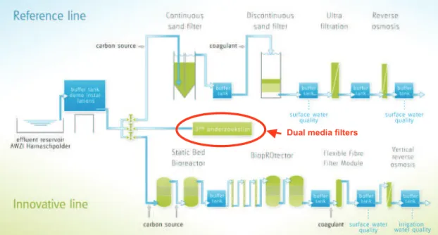
Most of the treated water goes through an underwater emissary to be ejected directly into the North Sea. About 50 m3/h of the final effluent goes to a research reclamation pilot, which consists of three research lines in
Dual media filters
Figure 2. Schematics of the Water Reclamation Pilot in the Harnaschpolder WWTP
1.4 Harnaschpolder’s (treated) wastewater parameters
Before the beginning of the filter experiments, an analysis of the Harnaschpolder’s WWTP waste‑ water was carried out. Samples were taken every week (using an automatic water sampler) and its components were analyzed (BOD, COD, DO, nitrates, carbonates, phosphates, sulphites, heavy met‑ als, alkalinity, turbidity, solids, etc.). The following table (Table 3) represents the annual average of the parameters:
Table 3. Harnaschpolder final effluent parameters
Parameter unit Avg Min. Max. measurementsNumber of
EC µS/cm 989 714 1180 4/49
TSS mg/l 7,38 0 110 301
TKN mg/l 2,13 1 8,8 301
NH4‑N mg N/l 0,58 0 3,81 206
BOD5 mg O2/l 3,28 1,4 24 301
COD mg O2/l 36,89 22 120 301
NO3‑N mg N/l 4,7 0 11 206
PO4‑P mg/l 0,49 0,11 3,06 206
total P mg/l 0,8 0,12 6,2 301
total N mg/l 6,83 1,86 13,3 301
Pb µg/l 2,48 0 7 20
Parameter unit Avg Min. Max. measurementsNumber of
Cr µg/l 1,21 0 13 20
As µg/l 1,23 0 5,4 20
Cu µg/l 0,83 0 10 20
Cd µg/l 0,05 0 0,9 20
Hg µg/l 0,03 0 0,3 20
Cl‑ mg/l 133,7 91 170 10
Ca mg/l 63,6 42 80,9 8
SO4 mg/l 62,5 48 72 4
Na mg/l 96,9 88,8 105 4
Mg mg/l 8,56 6,3 10,2 8
K mg/l 23 20,9 25,1 4
Hardness mmol/l 2,12 1,48 2,36 8
In the following table (Table 4), there are the quality demands (according to the Dutch quality standards) for greenhouse‑type waters.
Table 4. Greenhouse water quality demands
Class 1 unit value Class 2 unit value
EGV µS/cm <500 EGV µS/cm <500
Ptot mg P/l <15 Ptot mg P/l <40
N‑NO3‑ mg N/l <100 N‑NO3‑ mg N/l <150
N‑NH4 mg N/l <10 N‑NH4 mg N/l <10
SO42‑ mg/l <15 SO42‑ mg/l <40
K mg/l <200 K mg/l <350
Ca mg/l <80 Ca mg/l <150
Mg mg/l <12 Mg mg/l <40
Fe µg/l <50 Fe µg/l <500
Mn µg/l <200 Mn µg/l <500
Zn µg/l <150 Zn µg/l <450
B µg/l <100 B µg/l <200
Cu µg/l <50 Cu µg/l <150
Al µg/l <10 Al µg/l <20
Cr µg/l <5 Cr µg/l <5
Pb µg/l <1 Pb µg/l <1
2. OBJECTIVES OF THE RESEARCH
The objectives of this research are:
• To make a review on the different mechanisms for the removal of heavy metals from treated urban wastewater;
• Simulate solubility curves for the following heavy metals: Cd, Cu, Ni and Zn in wastewater with a physicochemical composition similar to the HNP treated effluent (heavy metals, alkalinity, pH, tem‑ perature, redox, nitrates and other ions, etc), using the PHREEQc computer simulation software; • Based on the lab‑scale results and the PHREEQc simulation, suggest possible physicochemical
removal mechanisms for heavy metals, from the Harnaschpolder WWTP effluent.
3. OVERVIEW OF THE RESEARCH
Stage Observations
1. Dimensioning & assembly of the filters at the HNP’s WWTP Pilot Installation.
Assembling the filters the best possible way, to prevent future leaks and/or other operational hazards. An operation and safety manuals were written in parallel to this practical stage.
2. Start ‑up Testing the system for possible leaks; adjust backwash system (air and fresh
water); adjust feeding system (keeping the influent flow steady).
3. First run («Blank run») Running the filters without addition being of heavy metals or carbon required for denitrification. Parameters such as turbidity, head loss, COD and NO3 – were
analyzed.
4. Heavy metal dosing Heavy metals such as Cd, Cu, Ni and Zn, were added to the filters with a
concentration of 250µg/L. Parameters such as turbidity, head loss, COD and NO3 –
and heavy metals were analyzed.
5. PHREEQc simulation Based on the physicochemical conditions present in the filters, solubility curves were simulated for the heavy metals studied in this research.
6. Results comparison Results from the experimental data (% of HM removal) and PHREEQc simutation
4. LITERATURE REVIEW
4.1 Heavy metal removal processes
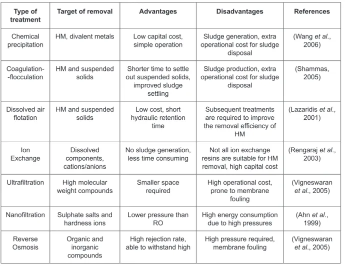
Facing with more and more strict regulations, heavy metal pollution is gradually becoming one of the most serious environmental problems. Therefore, toxic heavy metals should be removed from the wastewater to protect both people and environment (Singh et al., 2004). Many methods can be used to remove heavy metal ions, which include chemical precipitation, ion‑exchange, biosorption, adsorption, membrane filtration, electrochemical treatment technologies, etc. Although there are a great variety of treatments available, they have their inherent advantages and limitations in their application (Table 5).
Table 5. Summary of the different possibilities of physicochemical removal for wastewater
Type of
treatment Target of removal Advantages Disadvantages References
Chemical
precipitation HM, divalent metals Low capital cost, simple operation operational cost for sludge Sludge generation, extra disposal
(Wang et al., 2006)
Coagulation‑
‑flocculation HM and suspended solids out suspended solids, Shorter time to settle improved sludge
settling
Sludge production, extra operational cost for sludge
disposal
(Shammas, 2005)
Dissolved air
flotation HM and suspended solids hydraulic retention Low cost, short time
Subsequent treatments are required to improve the removal efficiency of
HM
(Lazaridis et al., 2001)
Ion
Exchange components, Dissolved cations/anions
No sludge generation,
less time consuming resins are suitable for HM Not all ion exchange removal, high capital cost
(Rengaraj et al., 2003)
Ultrafiltration High molecular
weight compounds Smaller space required High operational cost, prone to membrane fouling
(Vigneswaran
et al., 2005)
Nanofiltration Sulphate salts and
hardness ions Lower pressure than RO High energy consumption due to high pressures (Ahn 1999)et al., Reverse
Osmosis Organic and inorganic compounds
High rejection rate,
able to withstand high High pressure required, membrane fouling (Vigneswaran et al., 2005)
– Dual media filtration
In the author’s experiments, primary Jar ‑tests were conducted to test the ability to remove the so ‑called «conventional» parameters and simultaneously removing heavy metals. For this experiments, standards solutions of HM were also made (Nickel: 1000mg/L, Zinc: 100mg/L, Copper: 100mg/L) to dose in the pilot’s effluent. The removal efficiencies for the HM were compared by subjecting to three different coagulants: poly aluminium chloride, ferric chloride and powdered activated carbon in order to promote co ‑precipation.
The results of HM removal with co ‑precipitation with aluminium showed a relatively high removal of copper (79%) and an extremely low removal for nickel (15%). The efficiency removal for zinc and cop‑ per were 38% and 20% respectively, when using ferric chloride as coagulant. The dosage of powdered activated carbon resulted in a removal efficiency of 95% for both zinc and nickel (Miska ‑Markusch, 2009).
The filter experiments were realized at Horstermeer Pilot installation at the WWTP in the Nether‑ lands. The pilot installation consisted of two dual media filters (upper layer: anthracite, 80cm height; lower layer: quartz sand, 40cm height), assembled to work in parallel (one of them used as a control). The flow rate in operation was set to 8m3/h (filtration rate 10m/h), resulting in filtration run times between 4h (initial
stage) and 24h (in a final stage).
In the experiments, a heavy metal solution containing copper, nickel and zinc was prepared from metal chlorides and dosed to maintain a concentration of 120 ‑150µg/L of each metal in the filters treating WWTP’s effluent.
Final concentrations of HM were measured in both filters through cuvette analyses. Methanol and coagulant were also dosed as a carbon source for denitrification (of the pre ‑existent bacteria in the wastewater) and chemical precipitation of phosphorus, respectively.
These experiments were then subjected to different conditions such as the dosing of methanol, dosing of coagulant and the duration of the experiments.
As a result, the removal efficiency of the fraction of the total inorganic copper (particulate form) reached as high as 92% when the filters were dosed with coagulant and methanol. The copper dissolved fraction was extremely low (25mg/L), compared to the other metals.
The measurements for nickel present remarkably different results for copper: the dual media filter did not retain the dissolved form and the highest removal efficiency was only 25% when subjected only to carbon dosing.
The major concentration of zinc is in dissolved form, the same as nickel, but is partly removed in the dual media filter with approximately 60% of efficiency (Miska ‑Markusch, 2009).
4.2 Heavy metal removal mechanisms
Chemical Precipitation
Chemical precipitation in water and wastewater treatment is the change in form of materials dis‑ solved in water into solid particles. It is widely used for heavy metal removal from industrial effluents because its relatively simple and inexpensive to operate (Ku and Jung, 2001). The forming precipitates can be separated from the water by sedimentation or filtration so that the final effluent can be appropri‑ ately discharged or reused (Fu and Wang, 2011).
Most metals are precipitated as hydroxides, but other methods such as sulfide and carbonate pre‑ cipitation are also used. In some cases, the chemical species to be removed must be oxidized or reduced to a valence that can then be precipitated directly.
The chemical equilibrium relationship in precipitation that affects the solubility of the component(s) can be achieved by a variety of means. One or a combination of the following processes induces the precipitation reactions in a water environment (Wang et al., 2006).
Despite having operational and economic advantages, i.e. it is very simple to introduce the chemical into the wastewater and it is very cheap to do so, there are some disadvantages to take into consideration. Firstly, this process generates toxic sludges that need special attention to dispose (e.g. these chemical sludges must be disposed in special landfills or incinerators). Thus, it will add an extra cost to the operation of the WWTP. This also applies for other chemical precipitation processes such as coagulation/flocculation.
– Hydroxide precipitation
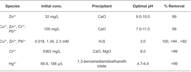
Hydroxide precipitation is the most widely used chemical precipitation technique, due to its relative simplicity, low cost and ease of pH control (Huisman et al., 2006). The solubilities of the various metal hydroxides are minimized in the pH range of 8.0 ‑11.0 for posterior removal by flocculation, sedimenta‑ tion or filtration processes. A variety of hydroxides has been used to precipitate metals from wastewater, based on the low cost and ease of handling, lime is the preferred choice of base used in hydroxide pre‑ cipitation at industrial settings (Baltpurvins et al., 1997) (Table 6).
Table 6. Heavy metals removal by using chemical precipitation (Fu and Wang, 2011)
Species Initial conc. Precipitant Optimal pH % Removal
Zn2+ 32 mg/L CaO 9.0 ‑10.0 99
Cu2+, Zn2+, Cr3+,
Pb2+ 100 mg/L CaO 7.0 ‑11.0 99
Cu2+, Zn2+, Pb2+ 0.018, 1.34, 2.3 mM H2S 3.0 100, >94 , >92
Cr3+ 5363 mg/L CaO, MgO 8.0 >99
Hg2+ 65.6, 188 µ/L 1,3 ‑benzenediamidoethaneth
Mirbagheri et al. (2005) studied the removal of hexavalent chromium from wastewater using cal‑ cium and sodium hydroxides. Results of their experiments showed that the maximum precipitation was obtained at a pH of 8.7 and the concentration of chromate was reduced from 30 mg/L to 0.01 mg/L (99% efficiency). Copper removal was also tested in the same experiments and the optimum pH for maximum precipitation was about 12, obtaining an efficiency of 98.5% (Mirbagheri and Hosseini, 2005).
In hydroxide precipitation process, the addition of coagulants such as alum, iron salts, and organic polymers can enhance the removal of heavy metals from wastewater.
Although widely used, hydroxide precipitation also has some limitations. Firstly, hydroxide precipita‑ tion generates large volumes of relatively low density sludge, which can present dewatering and disposal problems (Kongsricharoern and Polprasert, 1995). Secondly, some metal hydroxides are amphoteric, i.e. react as an acid as well as a base, and the mixed metals create a problem using hydroxide precipitation since the ideal pH for one metal may put another metal back into solution.
Thirdly, when complexing agents are in the wastewater, they will inhibit metal hydroxide precipitation.
– Sulfite precipitation
Sulfide precipitation is also an effective process for the treatment of heavy metals ions. Both «soluble» sulfides such as hydrogen sulfide or sodium sulfide and «insoluble» sulfides such as ferrous sulfide may be used to precipitate heavy metal ions as insoluble metal sulfides (Wang et al., 2006). The main advantage of using sulfides is that the solubilities of the metal sulfide precipitates are dramatically lower than hydroxide precipitates and sulfide precipitates are not amphoteric. This translates in a higher degree of metal removal over a broad pH range when compared with hydroxide precipitation. Also, the sludges formed in sulfite precipitation exhibit better thickening and dewatering characteristics than the corresponding metal hydroxide sludges.
Kousi et al. (2007) developed a new precipitation process based on sulfate ‑reducing bacteria (SRB), which consisted in oxidizing simple organic compounds, under anaerobic conditions, and trans‑ forming them into hydrogen sulfide. The hydrogen sulfide then reacts with divalent soluble metals to form insoluble metal sulfides, according to the following equation:
M2+(aq) + H2S (g) → MS (s) ↓ + 2H+(g)
According to the authors’ experiments, who developed an upflow fixed ‑bed SRB filter to monitor for the treatment of zinc ‑bearing wastewater, it was proved that this type of reactor has a considerable capac‑ ity of completely reducing sulfates with a maximum removal efficiency of 93% of zinc (Kousi et al., 2007). Despite the obvious advantages, there are also potential dangers in the use of sulfide precipitation process regarding the release of toxic H2S fumes, when the HM ions are subjected to acid conditions.
Moreover, metal sulfide precipitation tends to form colloidal precipitates that cause some separation problems in either settling or filtration processes.
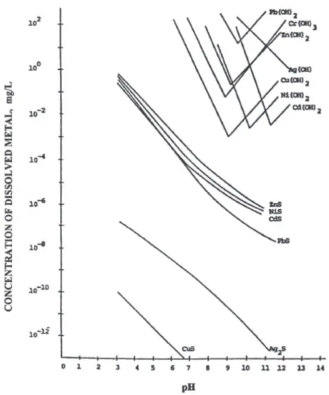
Figure 3. Solubility of hydroxides and sulfides as a function of pH (Wang et al., 2006)
In the graph above, it is clear that metal sulfides have lower solubilities than hydroxides, in the alkaline pH range, and also tend to have low solubilities at or below the neutral pH value. This means that in higher pH values, heavy metals precipitate mostly in the form of hydroxides rather than sulfides.
– Carbonate precipitation
– Cyanide precipitation
Cyanide precipitation, although a method for treating cyanide in wastewater, does not destroy the cyanide molecule, which is retained in the sludge that is formed. Reports indicate that during exposure to sunlight, the cyanide complexes can break down and form free cyanide. For this reason the sludge from this treatment method must be disposed of carefully. Cyanide may be precipitated and settled out of wastewater by the addition of zinc sulfate or ferrous sulfate, which forms zinc ferrocyanide or ferro – and ferri ‑cyanide complexes. In the presence of iron, cyanide will form extremely stable cyanide complexes (Wang et al., 2006, Botz et al., 2005).
– Heavy metal chelating precipitation
This occurs when organic molecules, containing more than one functional group with donor elec‑ tron pairs, can simultaneously donate these to a metal atom, forming a ring structure. In general, since a chelating agent may bond to a metal ion in more than one place simultaneously, chelated compounds are more stable than complexes involving monodentate ligands. Stability tends to increase with the number of chelating sites available on the ligand. Thus chelation of metals by donor ligands of biopolymers leads to the formation of stable species (Tsezos, 2007). The use of this mechanism in wastewater treatment is an economically viable alternative since commercial heavy metal precipitants today either lack the neces‑ sary binding sites or pose too many environmental risks to be safely utilized, compared to synthesized chelating agents (Matlock et al., 2002).
– Bio ‑precipitation
The selective sequestering of metal soluble species that result in the immobilization of the metals by microbial cells is also known biosorption (Tsezos, 2007). It results on the binding of metals and metal‑ loid species, compounds and particulates from solutions to functional groups on the cell surface polymers (Diels et al., 2003) (Wang and Chen, 2009).
Biosorption is a process with some unique characteristics. It can effectively sequester dissolved metals from very dilute complex solutions with high efficiency. This makes biosorption an ideal can‑ didate for the treatment of high volume low concentration complex wastewaters (Tsezos, 2007). The mechanisms that occur in biosorption mechanisms are similar to the physicochemical mechanisms which include: complexation, where metal ions are binded with organic molecules, involving the ligand centres in the organic species (Avery and Tobin, 1993) and micro ‑precipitation, where the precipitates may be formed and remain in contact with or inside the microbial cells or may be independent of the solid phase of the microbial cell (Remoudaki et al., 2003).
could lead to a chemical precipitation of heavy metals as hydroxides (Remoudaki et al., 2003, Hussein
et al., 2005).
– Chemical Adsorption
Adsorption has been successfully applied for treating municipal and drinking water. Successful removal of heavy metals from aqueous solutions using, for example, activated carbon has recently been demonstrated (Barakat, 2011, Bansal et al., 1988). Chemical adsorption is considered one of the best available technologies for eliminating non ‑biodegradable and toxic organic compounds from aqueous solutions, such as heavy metals (Benjamin et al., 1982). Its inherent physical properties such as a large surface area (500 ‑2000 m2/g), porous structure, high adsorption capacity and extensively reactive sur‑
face, make it extremely versatile (Barakat, 2011).
Solids with oxide surfaces can act as weak acids and bases in solution. The surface ions function as ion exchange sites. While increasing the pH, the adsorption of cations increases and adsorption of anions decreases. The adsorption capacity will change from 0% to 100% of the adsorbent’s total capacity over a narrow range of one or two pH units. (Leyva Ramos et al., 2002).
Complexing agents can either increase or decrease adsorption. They may decrease adsorption by stabilizing the ion in solution.
Alternatively, they may increase it by forming complexes that adsorb stronger than the ion alone. For example, cyanide can strongly increase adsorption of nickel ions at high pH values (Petrov et al., 1992, Marzal et al., 1996).
– Denitrification and heavy metals removal
Secondary effluents from wastewater treatment plants still contains several microorganism includ‑ ing heterotrophic organism, which are able to denitrify and remove nitrate nitrogen NO3 ‑N, when an
electron donor is present.
Biological denitrification involves the biological oxidation of many organic substrates in wastewater treatment using nitrate as the electron acceptor instead of oxygen. In biological nitrate reduction process, the electron donor is typically one of the three sources:
(1) the COD in the influent wastewater;
(2) the COD produced during endogenous decay;
(3) an exogenous source such as methanol or acetate (Metcalf & Eddy et al., 2003).
Alkalinity is produced in denitrification reactions and the pH is generally elevated (Metcalf & Eddy
through batch experiments. As a result, it was revealed that in the presence of both nitrate and sulphate, denitrification was the dominant process affecting metal behavior (Davis et al., 2007, Vanbroekhoven
et al., 2007). In addition, the removal of Cd and Zn in the presence of an electron acceptor (nitrate) with and without carbon source (acetate) was tested in column experiments, consequently it was concluded that the metals removal efficiency went up to close to 100% for both cases, however the mechanism of removal were different.
4.3 PHREEQc Software Simulation
PHREEQC is a software for simulating chemical reactions and transport processes in natural or polluted water. The program is based on equilibrium chemistry of aqueous solutions interacting with minerals, gases, solid solutions, exchangers, and sorption surfaces, but also includes the capability to model kinetic reactions with rate equations that are completely user ‑specified in the form of Basic state‑ ments. Kinetic and equilibrium reactants can be interconnected, e.g. by linking the number of surface sites to the amount of a kinetic reactant that is consumed (or produced) during the course of a model period.
PHREEQC is based on the Fortran program PHREEQE (Parkhurst et al., 1990), capable of simu‑ lating a variety of geochemical reactions for a system including:
• Mixing of waters;
• Addition of net irreversible reactions to solution;
• Dissolving and precipitating phases to achieve equilibrium with the aqueous phase;
• Effects of changing temperature, ion ‑exchange equilibrium, advective transport, surface‑ ‑complexation equilibrium and much more.
The numerical method has been modified to use several sets of convergence parameters in an attempt to avoid convergence problems. User ‑defined quantities can be written to the primary output file and (or) to a file suitable for importation into a spreadsheet, and solution compositions can be defined in a format that is more compatible with spreadsheet programs.
– Software potential in water and wastewater treatment
PHREEQc is generally used for water chemistry in geo ‑hydrology but hardly applied in water treat‑ ment, mainly because of the absence of scientific literature/educational material on water treatment with PHREEQc (Moel et al., 2011).
• Batch ‑Reaction Modeling – applied to problems in laboratory, natural, and contaminated sys‑ tems. The reaction capabilities of PHREEQc have been used frequently in the study of mine drainage, radioactive decay, etc.
• Speciation Modeling – useful in situations where the possibility of mineral dissolution or pre‑ cipitation needs to be known, as in water treatment, aquifer storage and recovery, artificial recharge, and well injection. It uses the chemical analysis of a water to calculate the distribution of aqueous species by using an ion ‑association aqueous model (Zhang et al., 2011). The results of speciation calculations are saturation indexes for minerals, which indicate whether a mineral should dissolve or precipitate (Charlton and Parkhurst, 2011).
To make all the calculations, the program uses various databases. The database file includes all the thermodynamic data used to make the saturation calculations and parameters for estimating the activity coefficients.
The «default» database of PHREEQc is «Phreeqc.dat», used for general purposes. The recom‑ mended database for water treatment is «Wateq4f.dat» (Moel et al., 2011), which result on the continuous compilation of information from literature and experimental data.
In this work, PHREEQc was used to calculate saturation indexes and distribution of the heavy metals in the filter medium (treated wastewater from the HNP WWTP and heavy metal dosing). The saturation indexes will then determine if the heavy metals will precipitate or stay dissolved in the solution, depending on the filters conditions (pH, temperature, alkalinity/acidity, redox, nitrates, sulfates, presence of other ions).
– Simulation of metal solubility as a function of pH from sludge samples
Using PHREEQc software, Remoudaki et. al (2003) simulated solubility curves of Nickel, Zinc and Copper, which indicate dominant insoluble species for the metals of interest (using «wateq4f. dat» as the main database), to make a comparison between the experimental data from bio ‑sorption sludges (containing high doses of HM) and the solubility curves at different pH values (with the same conditions as the experimental data). This helped to understand the mechanisms involved inside the filter medium.
In his experiments, the three heavy metals were selected taking into account the anions present in the sampled wastewater that can form insoluble species with the metal ions (cations) in the filter envi‑ ronment.
Figure 4. Zinc solubility diagram as function of pH
Figure 5. Nickel solubility diagram as function of pH
From the figures above, it is observed that the most soluble species are metal ‑carbonates (M ‑CO3)
since they have the highest equilibrium soluble concentrations in all three metals (copper, nickel and zinc). Metal phosphates are also very soluble comparing to the remaining phases.
5. MATERIALS AND METHODS
5.1 PHREEQc Simulation
As referenced before, PHREEQc has a large potential for application in water treatment. In its basic form all relevant chemical equilibriums for water chemistry are incorporated, including all redox reactions.
For this simulation, the «user friendly» of PHREEQc software was used (version 2.18.3 ‑5570 from the US Geological Survey), also called «PHREEQc Interactive».
– Development of the input file
PHREEQc software uses the keyword «SOLUTION» and «SOLUTION_SPREAD» for input of ele‑ ments in the solution. It uses chemical elements, such as Ca, H, O, Na, and C as prime input parameters. These elements might be subdivided into redox states of an element, such as C(+4) and C( ‑4) or Fe(+2) and Fe(+3). The elements and their definitions are relatively easy to insert into the program and they are given by different databases that comes with the software (Figure 7).
PHREEQc uses the «mole» as the default quantity for elements and «kg» (or kgw – quilo‑ grams of water) as the default quantity for the solvent. The amount of substance for an element in solution is calculated from its molal concentration (molality in mol/kgw) and the mass of water (by default 1 kg).
The elements H and O have a special status in PHREEQc because of their multiple appearances (H2O, H+, OH ‑, O2, H2) in the solution, and H2O being the solvent in PHREEQc.
In PHREEQc the speciation of elements is calculated from the pH and pe value (activity of each specie). The activity is a measure of the «effective concentration» of a species in a mixture, meaning that the species’ chemical potential depends on the activity of a real solution in the same way that it would depend on concentration for an ideal solution.
The pe value is calculated from the redox couple (in the database) if it is not directly specified in the input file.
Figure 7. Main screen of PHREEQC, with the SOLUTION keyword dialog box open.
– Writing the input file
In order to simulate a reaction between the influent (treated wastewater, containing traces of HM’s and other substances) and the HM mother solution (concentrated solution of heavy metals that is pumped into the filter), the input file was separated in five different steps:
SOLUTION 1 – Filter’s influent (HNP’s WWTP treated wastewater)
SOLUTION 2 – Heavy metals solution (containing heavy metal chlorides’ solution)
SOLUTION 3 – Fictitious solution that results in the mix of the previous solutions
EQUILIBRIUM PHASES – Simulates the equilibrium phase of each form of heavy metal,
i.e. verifies if any available form of heavy metal forms a precipitate.
REACTION – Addition of a base (NaOH) to simulate the variation of the heavy metals pre‑ cipitates solubility, according to the pH. Sodium hydroxide was (virtually) added instead of an acid, because the effluent was slightly acidic.
Firstly, the average values of Harnaschpolder’s WWTP effluent were inserted into «SOLUTION 1» (Table 7).
The database was set to «llnl.dat» (instead of «wateq4f.dat» used in Remoudaki’s experiments) because it is the most complete database regarding the information about all known inorganic aqueous species and minerals, especially heavy metals.
Table 7. Physicochemical parameters used in SOLUTION 1
Parameter Value* Unit
Temperature 19 ºC
pH 6.52 ‑
COD 35 mg/L
NH4 0.5 mg/L
NO3 4.4 mg/L
TSS 2.9 mg/L
Ni (dissolved) 18 µg/L
Zn (dissolved) <18 µg/L
Cd (dissolved) 0.3 µg/L
Cu (dissolved) 2 µg/L
Pb (dissolved) 8.2 µg/L
* average values of HNP’s treated effluent, retrieved from Delfluent website (www.delfluent.nl)
After introducing the initial solutions, both solutions were «virtually» mixed, at a ratio of 0.90/0.10,
i.e. a fraction of 0.90 is taken from the first solution while a fraction of 0.10 was taken from the second solution, generating another solution (SOLUTION 3). This ratio is very important because the flows are not equal, meaning that the feeding flow (wastewater) is 90% bigger than the heavy metal dosing flow. Finally, the reaction between the sodium hydroxide (strong base) and the resulting solution was intro‑ duced into the input file along with the possible precipitate forms of each heavy metal (e.g. for Copper: azurite, malachite, Cu(OH)2, etc.). Pressing the «Calculate» button, PHREEQc calculates the concentra‑
tion of each type of (possible) precipitate, under the operating conditions.
– The output file
The output of PHREEQC is a huge collection of calculated values, which lacks easy access for user specific information. The values in the output have been automatically converted into the units of the experiments.
Table 8. PHREEQc output section
Output section Description Main purpose
Solution composition Molality and moles for all elements3 Input check
Description of solution General parameters4 Calculated overall parameters
Redox couples1 pe and redox potential for all redox couples Electron balance in input
Distribution of species Molality, activity and gamma of all species,
with total molality per redox state of an element5 Speciation
Distribution of alkalinity2 Contribution in alkalinity per dissolved specie,
with molality and Acid ‑base buffering
Saturation indices SI, IAP and K values for all phases Relation to gas and solid
phases
1 Only in initial calculation, when unbalanced redox couples are present 2 Only in output if –alkalinity=true under PRINT
3 For initial calculation: including molality and moles for inputted redox states 4 For initial calculation: including Total CO2, if Alkalinity is in the input
5 For initial calculations: for elements with multiple redox states only the inputted redox states
5.2 Filter operation
Two dual media filters were assembled and started up in the wastewater reuse pilot at Harnas‑ chpolder WWTP. The filters were assembled and started up, for a further evaluation on removal of Cd, Cu, Ni and Zn (carried out through a parallel research).
In a first stage, two identical columns were operated in parallel under the same operational condi‑ tions (i.e. same feeding flow, outflow, hydraulic retention times, etc.). In a second stage, maintaining the same operational conditions, both filters were dosed with specific concentrations of Cd, Cu, Ni and Zn so that the removal efficiencies of these heavy metals could be compared with solubility curves simulated by PHREEQc. The last two experiments were also subjected to the same operational conditions as the first stage.
During all the stages, an ion exchange system was required to make sure that the effluent of these filters remained clean and metal ‑free, to meet the discharge guidelines.
Besides the removal of heavy metals, COD, NO3 – and turbidity as well as the influence of pH were
evaluated in a parallel work (Villarroel Toral, 2011).
– Filters set ‑up
The filters, operated in parallel, consisted of two down flow columns of manual control.
pump
Centrifugal
Flow meter
w/ ball
Bypass
Figure 8. Detail of the feeding system
The filter columns, made of transparent acrylic, were 3m high (in total) and had an internal diam‑ eter of 13 cm. The filter bed area is 0.013m2. The effective sand and anthracite bed heights were 105cm
and 45cm respectively. The effective height was 2.0m and the filter bed area as shown in Figure 10.
Figure 10. Detail of the filter column (values in cm)
The filter bed was filled with a bottom layer of sand with a diameter between 1.5 – 2.5 mm, with a density of 1600 kg/m3 and with a top layer of anthracite with grain diameter of 2 – 4 mm and, a density of
700 kg/m3. The filters, the flow meters and also other translucid or transparent equipment were covered
to prevent unwanted biomass growth.
A pressure gauge, a feeding pump (for wastewater), a head loss regulator, a HM dosing system (for individual dosing, also for carbon dosing) connected to peristaltic pumps (Watson ‑Marlow 200 series) and fresh water and air connections (for backwash) were made for each filter.
In the Figure 8 it is possible to see the different solutions for the feeding system that were tested during the start ‑up phase:
• Centrifugal pumps: they pump the treated wastewater from the HNP Pilot Buffer Tank (main tank that receives a very small percentage of the WWTP’s final/treated effluent) directly to the filters. The flow is then regulated though a ball ‑valve system.
• By ‑Pass: since the Pilot Buffer tank was elevated, it had enough pressure to feed the filters without using the (feeding) pumps. Thus, reducing the energy consumption and guarantees a more constant pressure.
Table 9. Dimensions and operational parameters of the lab ‑scale filters
Dimensions and operational parameters Value Unit
Diameter 0.13 m
Filter height 2.00 m
Sand bed height 1.50 m
Sand porosity (Φ) 1.4 – 2 mm
Feeding velocity rate: 5 to 15 m/h
Backwash velocity rate: 15 to 75 m/h
Starting point backwash*: 1.5 min with air, 1 min (air+water), 0.5 min water
* theoretical times, according to Miska ‑Markusch (2009)
The filters were initially assembled according to Figure 11, which give a simples description of the setup for an easy understanding of their operation. The filters setup was constantly modified in order to comply with several safety, operational and practical restrictions that were imposed at the HNP’s Pilot Plant.
Throughout the design process of the lab scale filters, several drawings were made in order to specify the direction and types of flows (wastewater inlets, clean water, compressed air, heavy metals, methanol, effluent, biomass), equipments (pumps, valves, tanks) and other details. These drawings are available in the «Appendix I» section.
The filters were firstly partially assembled at TU Delft’s sanitary engineering lab’s to make sure everything was water tight. After checking the filters, they were brought to Harnaschpolder’s Pilot Plant for the final assembly (Figure 12).
Figure 12. Filters assembly at Harnaschpolder’s Pilot Plant
33
Figure 13. Schematics of the setup for the filtration experiments
To feed each of the dual media filters (labeled as «filter A» and «filter B») two peristaltic pumps were installed. The inlet of each filter was located at 50cm from the top, which was at 250cm of height.
As the feeding water gets into the filter, it moves downwards throughout the filter media into the sewage system (effluent outlet). The outflow (effluent) can be simply altered by regulating the height of the effluent discharge, to prevent that the filter dries. The filter effluent was then treated by ion exchange before being discharged on the sewage to make sure that no heavy metals would pollute the effluent line.
Figure 14. Effluent regulator box
– First run of experiments – «start up»
The «start up» is a very important procedure in order to understand the optimal combination of fil‑ ter bed depth, particle size (depends of the filter material), filtration velocity and height of the supernatant water (head loss).
Table 10. Summary of effects of independent variables on length of filter run (Miska ‑Markusch, 2009)
Independent Variable
Head loss Effluent Quality
Time Cumulative volume Time Cumulative volume
Depth ↑ ↓ ↓ ↑ ↑
Media Size ↑ ↑ ↑ ↓ ↓
Velocity ↑ ↓ ↔ ↓↓ ↓
Influent Conc. ↑ ↓ ↓ ↓ ↓
During the start ‑up of the filters there were a few problems: the filters were fed by two centrifugal pumps which were not capable to keep a constant flow into the filters. After trying higher flow rates and pump adjustments, the problem was solved by replacing the centrifuge pumps by peristaltic pumps, that are more reliable.
The dosing of heavy metals in both filters was only done after two months of practical adjustments required to solve leakages and desired pumping flows.
– Filters backwash
At the maximum achieved water level, the maximum filter resistance and turbidity are reached. The dual media filters were backwashed with both air (at 3bar of pressure) and water (more than 2m of pressure). Before every backwash, all the influent connections were shut down and the respec‑ tive valves were closed. The backwash procedure started firstly with 1 ‑1.5 minutes of air; then the air supply was closed and then the filter was washed with tap water with a flow rate between 700 and 1000 L/h for 5 minutes. During the backwash with tap ‑water, air at low flow can also be applied in case of heavy bulking on the top of the filters. The backwash effluent was sent to a buffer tank, followed by ion exchange, before final discharge. Figure 15 presents the backwash system assembled in the lab scale pilot installation.
– Heavy metals dosing and measurements
The dosing of heavy metals was done directly in the feeding pipe from a high concentrated solution of heavy metals that was replaced every two or three days.
The high concentrated solution was prepared with metal chloride compounds in order to obtain final concentrations in the filter of 250μg/L of each metal (Ni, Cd, Cu and Zn).
Table 11 shows the composition of the mother solution that was pumped into filter at 1,25mL/min flow rate, through a peristaltic pump (Watson Marlow Series 200).
Table 11. Heavy metals concentration for mother solution
HM Metal Chloride Qfilter
HM concentration in
the filter Qdosing pump
Metal
concentration of Metal*Fraction
Metal Chloride in mother
solution
‑ L/h μg/L mg/L L/h mL/min mg/L ‑ mg/L
Cd CdCl(n=0.5 ‑2.5)2.nH2O 100 250 0.250 0.075 1.25 333.33 0.492 677.03
Cu CuCl2.2H2O 100 250 0.250 0.075 1.25 333.33 0.373 894.11
Ni NiCl2.6H2O 100 250 0.250 0.075 1.25 333.33 0.247 1349.38
Zn ZnCl2 100 250 0.250 0.075 1.25 333.33 0.480 694.84
* Fraction of pure metal that is contained in the metal chloride powder
The total and dissolved concentrations of heavy metal (Cd, Cu, Ni and Zn) were determined (in a parallel research) by means of Inductively Coupled Plasma (ICP ‑MS) for both filters, in three sampling points: input, filtrate and at 85cm bed height (beginning of anthracite layer). A daily composite sample from the input and filtrate were taken for characterization. Also, the COD and NO3 consumption were
analyzed in the filters by cuvette tests. The pH, temperature and turbidity concentration were measured as well by hand analyzers. The samples were taken immediately to the water lab located in HNP treat‑ ment plant to be analyzed (Table 12).
Table 12. Physicochemical parameters measured in the filters
Parameters Units
pH ‑
Turbidity NTU
Temperature ºC
COD mg/L
The head loss along the dual media filter was also recorded by reading the pressure variation in the manometers located at the side of each filter column.
– Filter operation
The filter operation was divided in two stages: a first stage (blank conditions) without any additions into the filter and a second stage were heavy metals were added. A third stage was further carried out with addition of heavy metals, carbon and metal sorbing bacteria but the analysis and results of this last stage are out of the scope of this research.
As mentioned before, the filters were operated at a constant flow and raised water level. A feed flow of 100 (±5) L/h was used for the operation of the filters, with filtration velocities between 8 and 25 m/h and a hydraulic retention time (HRT) of approximately 10 minutes. During the run time of the filters, the removal of solids and the accumulation of biomass took place on the top layer, as a consequence the filter resistance increased leading to the backwash of the system.
I. First stage: Blank conditions
The filters were run without any additions (heavy metals, carbon) for some weeks. During this period, the turbidity, pressure (head loss), COD and NO3 was controlled every day for 4 days. The aim
of this stage was to check that both filters (A and B) would present the same efficiency since they were operated under the same conditions.
The filter run time (Tr) for this stage was 4 days and the SWL increased to a maximum of 260 cm. The applied backwash consisted of 5min of tap water at a flow rate of 1000 L/h. Because there was no introduction of HM into the filters, the backwash water was directly discharged in the sewerage system.
II. Filters with addition of heavy metals
After stabilization of both filters as a first stage, Filter A and B were dosed in order to present 250 μg/L of each metal (Cd, Cu, Ni and Zn) in the filter.
Heavy metals, turbidity, COD, NO3 ‑N, pH and temperature were monitored as in the previous
stage.
6. RESULTS AND DISCUSSION
6.1 Results obtained using PHREEQc software
The possibility of metals precipitation during filter experiments was tested to estimate the circum‑ stances in which metal precipitation takes place. Using PHREEQc software, solubility diagrams were then created for each heavy metal in which is represented various solubility curves for each phase of the same metal. The metals used in this simulation represent the ions that are most commonly found in the Harchaspolder’s untreated and treated effluent.
– Cadmium equilibrium diagram
The following graph shows the cadmium solubility curves for cadmium (Cd) complex included in the simulation (Figure 16). These metal complexes are manually selected from the program’s own database (in this case is the «llnl.dat»). The same procedure was done for the remaining heavy metals.
The yy axis represents the variation of concentration of the cadmium phases while the xx axis represents the variation of pH. Sodium hydroxide was “virtually” dosed to simulate the variation of pH in this graph (Figure 16).
The cadmium phases that are most likely to precipitate under the filters conditions are cadmium hydroxide (Cd(OH2), cadmium carbonate (CdCO3 , also known as «otavite»), cadmium sulfite (CdS) and
cadmium phosphate (Cd3(PO4)2).
Figure 16. Cadmium equilibrium diagram
On the other hand, the other two forms of cadmium present in this «mixed water» – cadmium hydroxide and cadmium carbonate – show possible precipitation from pH above neutrality, which means that they only precipitate in alkaline environments, according to the graph above. According to the graph, cadmium carbonate starts to precipitate from pH values close to 8.5, reaching maximum precipitation at pH=9.75 (approximately) and ceasing to precipitate at pH=11 (approximately). However, cadmium hydroxide only precipitates at pH values greater than 11, meaning that these two species don’t coexist in the solution. Maximum precipitation (for cadmium hydroxide) is achieved at maximum pH levels possible (12 < pH < 12.25). The results obtained in this simulation are coherent with the bibliography (chapter 3, Figure 3), which confirms that the cadmium hydroxides do precipitate in the presence of alkaline solu‑ tions (pH=11 ‑12).
According to the filter analysis during the first stage of the filter operation, a removal of 86% for this metal was achieved. This suggests that the removal observed in the filters was mostly physicochemical rather than biological. With no inoculation of bacteria in the filters nor carbon source it is very unlikely to remove HM biologically.
However, since the pH of the HNP effluent was slightly acidic, most of the removal wasn’t caused by physicochemical precipitation but by another process probably by adsorption in the anthracite layer, according to the bibliography (Benjamin et al., 1982).
In the filters with inoculation of heavy metals (and carbon), when carbon is metabolized by the bacteria is generates alkalinity, thus increasing the pH and promoting chemical precipitation. However, the pH values in the filter remained largely constant at 6.85 meaning that metal precipitation mechanisms (as metal hydroxides and carbonates) are unlikely to occur in the operating conditions.
The simulation showed that possible precipitation occurred at high levels of pH, i.e. in an alkaline environment. However, during the filter operation, the pH remained slightly under the neutrality (6.85) and there were no «optimal conditions» for occurring chemical precipitation of cadmium.
This way, the removal occurred in the filter suggests that there were involved some adsorption mechanisms into the filter material or into the bacteria already present in the wastewater that may serve as an adsorbent.
– Copper equilibrium diagram
The following graph shows the copper solubility curves for each complex of copper that can be formed with the ions present in the wastewater.
The yy axis represents the variation of concentration of the copper phases while the xx axis rep‑ resents the variation of pH. Like the previous graph (cadmium), sodium hydroxide was «virtually» dosed to simulate the variation of pH in this graph (Figure 17).
Unlike cadmium, some phases of copper such as carbonates and hydroxides appear together in the same compound, under certain conditions; i.e. minerals such as «azurite» (Cu3(CO3)2(OH)2) and
«malachite» (Cu2CO3(OH)2) may be formed according to the simulation. The remaining forms that were
Figure 16. Copper equilibrium diagram
According to the graph above, it is clear that most of the copper phases don’t have any reaction, under the simulation conditions; i.e. their solubility remains unchanged while pH increases gradually. The majority of the forms shows no changes in their solubility for all the pH range, meaning that these three phases remain soluble (high concentration solubility values) regardless of the pH variation in the final solution.
On the other hand, the only form of copper present in this «mixed water» appears to be «mala‑ chite» (the grey line), where possible precipitation starts slightly above the neutrality point (pH=7.25, approximately) and the solubility decreases along the increase of pH. Precipitation achieves maximum values at pH of 9.5‑10 and decreases gradually until achieves a maximum pH of approximately 11, according to the graph.
According to the bibliography in the «Literature Review» chapter, the results obtained in this simu‑ lation are discordant. The precipitation of copper hydroxide (or «malachite»),in the graph above, is similar to the chemical precipitation portrayed in the literature review. According to Wang et al. (2006), the pre‑ cipitation of copper hydroxide compounds occurs in a pH from 6 to 12. This compound is most insoluble when pH values are near 9 ‑10 (Wang et al., 2006), which also happens in the simulation.
On the other hand, «covellite» (or copper sulfite), according to the literature, which tends to pre‑ cipitate at an optimal pH of 6.8 doesn’t show any difference in the solubility curves in the simulation. This may point out the fact that other processes of copper precipitation may be involved in the simulation like adsorption into the filter or maybe adsorption into the bacteria.