Validation of ozone monthly zonal mean profiles obtained from the Version 8.6 Solar Backscatter Ultraviolet algorithm

(1)

ACPD

13, 2549–2597, 2013

Validation of ozone monthly zonal mean profiles obtained from the v8.6 SBUV

N. A. Kramarova et al.

Title Page

Abstract Introduction

Conclusions References

Tables Figures

◭ ◮

Back Close

Full Screen / Esc

Printer-friendly Version

Interactive Discussion

Discussion

P

a

per

|

Dis

cussion

P

a

per

|

Discussion

P

a

per

|

Discussio

n

P

a

per

|

Atmos. Chem. Phys. Discuss., 13, 2549–2597, 2013 www.atmos-chem-phys-discuss.net/13/2549/2013/ doi:10.5194/acpd-13-2549-2013

Atmospheric Chemistry and Physics Discussions

This discussion paper is/has been under review for the journal Atmospheric Chemistry and Physics (ACP). Please refer to the corresponding final paper in ACP if available.

Validation of ozone monthly zonal mean

profiles obtained from the Version 8.6

Solar Backscatter Ultraviolet algorithm

N. A. Kramarova1, S. M. Frith1, P. K. Bhartia2, R. D. McPeters2, S. L. Taylor1, B. L. Fisher1, G. J. Labow1, and M. T. DeLand1

1

Science Systems and Applications Inc., Lanham, MD, USA

2

NASA Goddard Space Flight Center, Greenbelt, MD, USA

Received: 16 November 2012 – Accepted: 9 January 2013 – Published: 24 January 2013

Correspondence to: N. A. Kramarova (natalya.a.kramarova@nasa.gov)

(2)

ACPD

13, 2549–2597, 2013

Title Page

Tables Figures

◭ ◮

Back Close

Full Screen / Esc

Discussion

P

a

per

|

Dis

cussion

P

a

per

|

Discussion

P

a

per

|

Discussio

n

P

a

per

|

Abstract

We present validation of ozone profiles from a number of Solar Backscatter Ultravio-let (SBUV and SBUV/2) instruments that were recently reprocessed using an updated (Version 8.6) algorithm. The SBUV data record spans a 41-yr period from 1970 to 2011 with a 5-yr gap in the 1970s. The ultimate goal is to create a consistent, well-calibrated

5

dataset of ozone profiles that can be used for climate studies and trend analyses. SBUV ozone profiles have been intensively validated against satellite profile measurements from the Microwave Limb Sounders (MLS) (on board UARS and Aura satellites) and the Stratospheric Aerosol and Gas Experiment (SAGE II) and ground-based observa-tions from the microwave spectrometers, lidars, Umkehr instruments and balloon-borne

10

ozonesondes. In the stratosphere between 25 and 1 hPa the mean biases and standard deviations are mostly within 5 % for monthly zonal mean ozone profiles. Above and be-low this layer the vertical resolution of the SBUV algorithm decreases. We combine several layers of data in the troposphere/lower stratosphere to account for the lower resolution. The bias in the SBUV tropospheric/lower stratospheric combined layer

rel-15

ative to similarly integrated columns from Aura MLS, ozonesonde and Umkehr instru-ments varies within 5 %. We also estimate drifts in the SBUV instruinstru-ments and their potential effect on the long-term stability of the combined data record. Data from the SBUV instruments that collectively cover the 1980s and 2000s are very stable, with drifts mostly less than 0.5 % yr−1_{. The features of individual SBUV(/2) instruments are}

20

discussed and recommendations for creating the merged SBUV data set are provided.

1 Introduction

As levels of chlorine and other ozone depleting constituents in the atmosphere stabilize and begin to fall, we expect stratospheric ozone values to begin to recover. Atmospheric chemistry models predict a slow recovery, with stratospheric ozone levels returning to

25

(3)

ACPD

13, 2549–2597, 2013

Title Page

Tables Figures

◭ ◮

Back Close

Full Screen / Esc

Discussion

P

a

per

|

Dis

cussion

P

a

per

|

Discussion

P

a

per

|

Discussio

n

P

a

per

|

(Strahan et al., 2011). To isolate long-term trend signals from natural ozone variations and quantify the rate of ozone recovery in observations, highly calibrated datasets are required. Several recent studies have demonstrated increases in stratospheric ozone at mid- and high- latitudes, which are marginally statistically significant (Newchurch et al., 2003; Yang et al., 2006), but longer data records are needed to verify and increase the

5

significance of these results. We rely on models to predict future ozone evolution, but those models must be validated using past and current observations to give confidence in their future results (WMO, 2011).

The Solar Backscatter Ultraviolet (SBUV) series of instruments provide the longest available record of global ozone profiles, with nearly continuous data over a 41-yr time

10

span, from April 1970 to the present, except for a 5-yr gap in the 1970s (McPeters et al., 2013). The dataset includes ozone profile records obtained from the Nimbus-4 BUV and Nimbus-7 SBUV instruments, and a series of SBUV(/2) instruments launched on NOAA operational satellites (NOAAs 9, 11, 14, 16, 17, 18 and 19). Four instruments are currently operational. In addition, the Ozone Mapper Profiler Suite (OMPS) – a

suc-15

cessor of the SBUV – was recently launched onboard the Suomi NPP satellite. Data from the OMPS instrument will be used to continue the 40 yr record of ozone obser-vations. OMPS observational data have been acquired since March 2012, and the instrument is performing well, exceeding its design requirements. While the calibration is still being finalized, the data are consistent with that from SBUV/2 instruments on

20

NOAAs 17, 18, and 19.

Although modifications in instrument design were made in the evolution from the BUV instrument to the modern SBUV/2 model, the basic principles of the measure-ment technique and retrieval algorithm remain the same (Bhartia et al., 2012). Each instrument makes nadir-viewing measurements of ultraviolet radiation scattered by the

25

(4)

ACPD

13, 2549–2597, 2013

Title Page

Tables Figures

◭ ◮

Back Close

Full Screen / Esc

Discussion

P

a

per

|

Dis

cussion

P

a

per

|

Discussion

P

a

per

|

Discussio

n

P

a

per

|

(DeLand et al., 2012). The homogeneity of measurements allows us to create a con-sistent, calibrated dataset of ozone profiles for use in climate study and trend analysis. However, to properly apply these data we must have a thorough understanding of the uncertainties in each instrument, and how these uncertainties translate to uncertain-ties in the combined record. For this purpose it is important to validate ozone profiles

5

obtained from each individual instrument against coincident satellite and ground-based measurements. Hereafter we will use “SBUV” to refer in general to all instruments and will specify individual instruments by their satellite name (for example, N9 refers to the NOAA 9 SBUV/2).

In this study we analyze the newly processed v8.6 SBUV profiles based on

com-10

parisons with a number of independent profile measurements. In Sect. 2 we provide a description of the SBUV version 8.6 dataset and correlative independent data and discuss the validation methods used. In Sect. 3 we estimate and analyze biases and standard deviations of the SBUV instruments relative to independent measurements in the stratosphere between 25 and 1 hPa. In Sect. 4 we validate the SBUV ozone

15

amounts in the thick layers with the corresponding amounts obtained from Aura MLS (250–25 hPa and 250–16 hPa), ozonesonde (surface-30 hPa) and Umkehr (surface to 30 hPa) measurements. In Sect. 5 we estimate drifts for each individual SBUV instru-ment relative to independent satellite and ground-based measureinstru-ments. In the final section we present conclusions, including recommendations we follow when

construct-20

ing the merged SBUV data set.

2 Data sets and methods

2.1 SBUV Version 8.6 Data

Several processing changes were made in Version 8.6. Brion-Daumont-Malicet ozone cross sections (Daumont et al., 1992; Brion et al., 1993; Malicet et al., 1995) were used

25

(5)

ACPD

13, 2549–2597, 2013

Title Page

Tables Figures

◭ ◮

Back Close

Full Screen / Esc

Discussion

P

a

per

|

Dis

cussion

P

a

per

|

Discussion

P

a

per

|

Discussio

n

P

a

per

|

derived from Aura OMI measurements (Joiner et al., 1995; Vasilkov et al., 2008), and a new ozone climatology based on the Aura MLS and ozonesonde observations (McPeters and Labow, 2012) have been implemented. Radiance adjustments in v8.6 were made for each instrument to maintain a consistent calibration, and ozone data for all instruments were reprocessed using adjusted radiances (DeLand et al., 2012). The

5

absolute radiance calibration for N14, N16, N17 and N18 were made relative to N17, while N7, N9 and N11 were calibrated against the Shuttle SBUV. Calibration for N4 is based on measurements at Arosa.

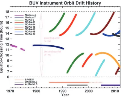
Figure 1 shows a timeline for SBUV instruments. The x-axis shows years, while the y-axis shows the equator-crossing local time (ECT). The first two instruments – N4 and

10

N7 – flew in stable near-noon ECT orbits. Instruments starting with N9 were launched on satellites with drifting orbits. When the orbit of an SBUV instrument approaches the terminator the quality of the measurements decline. It is not clear why this occurs (Bhartia et al., 2012), but most likely it is due to instrumental problems that increase at high viewing angles (DeLand et al., 2012). The first three SBUV/2 instruments launched

15

on NOAA satellites (N9, N11 and N14) began drifting rapidly shortly after launch. The onset of orbit drift is slower for the more recent instruments, starting with N16.

The v8.6 algorithm uses the Optimal Estimation technique (Rodgers, 2000) to re-trieve ozone profiles as ozone layer amounts (partial columns, DU) in 21 pressure layers. This is the same algorithm used in the previous Version 8 processing. The

cor-20

responding total ozone values are calculated by summing ozone columns at individual layers.

For the first time we are releasing the SBUV monthly zonal mean (mzm) ozone profiles as a primary product in addition to the more familiar level 2 PMF files. The SBUV v8.6 mzm time series are best suited for long-term trend analysis rather than

25

(6)

ACPD

13, 2549–2597, 2013

Title Page

Tables Figures

◭ ◮

Back Close

Full Screen / Esc

Discussion

P

a

per

|

Dis

cussion

P

a

per

|

Discussion

P

a

per

|

Discussio

n

P

a

per

|

bins with midpoints starting at 87.5◦_{S. To create mzm profiles all ozone profiles are}

screened to ensure high quality, and only profiles with an error flag of 0 (no flag) or 1 (solar zenith angle in the 84–88◦range) are accepted. We also require that the mean latitude of measurements within each latitude band are within 1 degree of the center of the band, and similarly that the mean time of measurements within a given month

5

is within 4 days of the center of the month (i.e. day 15). Data have been averaged for either the ascending phase of the orbit or the descending phase of the orbit, whichever gives the best coverage. A volcano contamination index (VCI) flag has been developed to identify potential aerosol contamination of the ozone measurements following the eruptions of El Chich ´on (April 1982) and Mt. Pinatubo (July 1991). The VCI flag uses

10

the absolute value of mzm ozone in layer 1 (639–1013 hPa) and the standard deviation of mzm ozone values in layer 10 (10.1–16.1 hPa) as indicators of possible contamina-tion. This flag is currently relevant for N7 SBUV data following the El Chich ´on eruption, but does not appear to properly capture the aerosol evolution in time and latitude fol-lowing the Mt. Pinatubo eruption. Therefore in our analysis we use the VCI as a filter for

15

N7 SBUV, and exclude all data after the eruption of Mt. Pinatubo through 1992 for N9 and N11. We note that N9 was in a near-terminator orbit when Mt. Pinatubo erupted, and the data are likely affected beyond 1992.

As part of the v8.6 processing we focused on estimating the various sources of error in the SBUV ozone retrievals using independent observations and analysis of the

algo-20

rithm itself (Bhartia et al., 2012; Kramarova et al., 2013). We found the main source of error in the SBUV profile retrievals is the smoothing error, which defines the error due to profile variability that the SBUV observing system cannot measure. Due to the low vertical resolution in the lower stratosphere and troposphere, SBUV measures a signal from a wide vertical range and the retrieval algorithm relies on the a priori

informa-25

(7)

ACPD

13, 2549–2597, 2013

Title Page

Tables Figures

◭ ◮

Back Close

Full Screen / Esc

Discussion

P

a

per

|

Dis

cussion

P

a

per

|

Discussion

P

a

per

|

Discussio

n

P

a

per

|

and below this range. The largest smoothing errors were found in the troposphere (up to 15 %). To minimize the SBUV smoothing e_ffect we recommend combining individual layers in the lower stratosphere and troposphere (Kramarova et al., 2013).

To facilitate analysis with the SBUV profile data, we provide the SBUV Integrated Ker-nel (IK) matrices, a priori profiles, weighting functions (Jacobian) and smoothing errors

5

in addition to the ozone mzm product. Having the error bars and retrieval characteris-tics along with ozone profiles makes it easier to analyze and properly use SBUV data (Kramarova et al., 2013). In addition to the layer data, SBUV profile ozone is reported as a mixing ratio at 15 fixed levels between 50 and 0.5 hPa. Ancillary data, including the number of profiles in the mzm average, the standard deviations, the average solar

10

zenith angles, and the total covariance matrices used to compute the smoothing error, are also included in the mzm files.

2.2 Independent satellite ozone profile measurements

We validate SBUV ozone mzm profiles against independent satellite measurements, obtained from the Stratospheric Aerosol and Gas Experiment II (SAGE II) instrument

15

and two Microwave Limb Sounder (MLS) instruments flown on the Upper Atmosphere Research Satellite (UARS) and Aura satellites. The timeframes for each independent satellite observation are shown on Fig. 1. In this section we provide brief description of each independent datasets.

2.2.1 SAGE II

20

The SAGE II instrument was launched in October 1984 and operated until August 2005. SAGE II uses the solar occultation technique to measure ozone, aerosol, nitrogen diox-ide, and water vapor profiles. The ozone is derived from the attenuation of solar radia-tion at 600 nm as it passes through the limb of the atmosphere (Mauldin et al., 1985). SAGE retrieves ozone vertical profiles with 1–2 km resolution from the upper

tropo-25

(8)

ACPD

13, 2549–2597, 2013

Title Page

Tables Figures

◭ ◮

Back Close

Full Screen / Esc

Discussion

P

a

per

|

Dis

cussion

P

a

per

|

Discussion

P

a

per

|

Discussio

n

P

a

per

|

and sunsets per day, resulting in profiles equally spaced in longitude along two narrow latitude bands. The poleward extent of the SAGE coverage varies with season, from 50 degrees in the winter hemisphere to 70 degrees in the summer hemisphere. The latitude of daily observations varies in time such that the full latitude range is covered ∼every 3 weeks.

5

We use both sunrise and sunset SAGE II data from 1985–1999. We do not con-sider SAGE II data after 1999 because they are limited to sunset events only. In this study we use SAGE II Version 6.2 data. Wang et al. (2002) assessed the quality of the SAGE V6.1 data and reported data precision of 4 % or better above 25 km, with less precision (10–50 %) at lower altitudes. Only minor changes (typically <0.5 %) to the

10

SAGE ozone were made in the update to SAGE V6.2 (http://www-sage2.larc.nasa.gov/ Version6-2Data.html). We apply filters to the SAGE profiles to account for aerosol and cloud contamination and other sporadic anomalous data as recommended by Wang et al. (2002).

2.2.2 UARS MLS

15

The first satellite-based Microwave Limb Sounder (MLS) instrument flew on the UARS platform, launched in September 1991 (Barath et al., 1993; Waters et al., 1993). The in-strument operated through August 1999, but the number of measurements decreased over time beginning in 1994 in an effort to limit antenna degradation and conserve instrument power. Ozone measurement noise increased after the shutdown of the

20

63 GHz channel in June 1997. The MLS instrument measures the thermal emission spectrum from the Earth’s limb at three wavelengths. In this study we use ozone re-trieved from the 205 GHz channel. The UARS orbit was such that measurements were made from 34 degrees in one hemisphere to 80 degrees in the other. Every 36 days the satellite underwent a 180 degree yaw maneuver, and the opposite hemisphere was

25

(9)

ACPD

13, 2549–2597, 2013

Title Page

Tables Figures

◭ ◮

Back Close

Full Screen / Esc

Discussion

P

a

per

|

Dis

cussion

P

a

per

|

Discussion

P

a

per

|

Discussio

n

P

a

per

|

and mesosphere. We use the version 5 data in the vertical range 64 hPa–1 hPa, and filter data as recommended by the instrument team (Livesey et al., 2003). UARS MLS measures at varying local solar times, day and night, but we use only daytime mea-surements for comparison with SBUV.

2.2.3 AURA MLS

5

The Aura satellite was launched in July 2004 with an MLS instrument on board, and the instrument continues to operate (Froidevaux et al., 2008). Aura MLS measures thermal limb emissions over five broad wavelength ranges using seven radiometers. The Aura orbit allows for uniform spatial sampling over the globe daily, and ozone profiles are retrieved from the 240 GHz spectral band. The AURA MLS vertical range is 200 hPa–

10

0.02 hPa, and covers a wider vertical range than the UARS MLS measurements. The vertical resolution of the instrument is _∼2.5 km throughout most of the profile, and the ozone is retrieved at a resolution of 12 levels per decade of pressure (_∼ about 1 km). We use the current version 3.3 MLS data set, and filter the data according to recommendations outlined in the MLS Version 3.3 users guide (Livesey et al., 2011).

15

For comparison with SBUV we use only daytime MLS measurements.

2.3 Independent ground-based ozone profile measurements

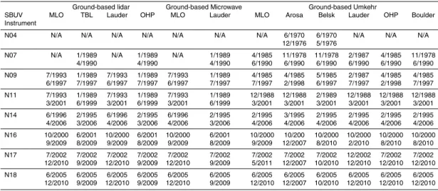
We validate SBUV measurements against three types of the ground-based ozone pro-filers: microwave spectrometers, lidars and Umkehr instruments. Here we summarize the main features of the based instruments. Table 1 shows the list of

ground-20

based stations and overlapping time periods with each SBUV instrument.

2.3.1 Microwave spectrometers

We use data from ground-based microwave spectrometers located at Mauna Loa, Hawaii, USA (20◦N) and Lauder, New Zealand (45◦S). The microwave spectrometers measure a spectral line produced by a rotational transition of ozone at 110.836 GHz.

(10)

ACPD

13, 2549–2597, 2013

Title Page

Tables Figures

◭ ◮

Back Close

Full Screen / Esc

Discussion

P

a

per

|

Dis

cussion

P

a

per

|

Discussion

P

a

per

|

Discussio

n

P

a

per

|

One of the advantages of the microwave spectrometers is their ability to operate unat-tended day and night, independent of weather conditions (Parrish et al., 1992). Mi-crowave profiles cover an altitude range of 56–0.1 hPa (about 20–66 km) with a vertical resolution about 8 km below 3 hPa and up to 17 km at 0.2 hPa. Net precision of the measurements is 4–6 % between 55 and 0.2 hPa (Connor et al., 1995). Regular

obser-5

vations at Mauna Loa and Lauder started in 1995 and 1992, respectively, and continue to date. We use daytime measurements only for comparisons with SBUV.

2.3.2 Lidar instruments

For our validation work we use data from four lidar instruments, located at Mauna Loa, Hawaii, USA (20◦N), Lauder, New Zealand (45◦S), Table Mountain, California,

10

USA (34.4◦N) and Haute Provence, France (44◦N). All four instruments are Differential Absorption Lidars (DIAL) and make measurements at both ozone absorbing (308– 338 nm) and non-absorbing wavelengths (355–387 nm) (McDermid et al., 1990). The lidars retrieve ozone profiles in the vertical range from approximately 20 to 50 km with a vertical resolution of about 0.3 km in units of number density (cm−3) on geometric

15

height (Megie et al., 1985). The lidars can operate only at night and depend on weather conditions. Thus the sampling at each station is distributed unevenly and at some sta-tions depends on season. We consider only lidar measurements with reported errors less than 10 %. The lidar stations started operating in the late 1980s (see Table 1 for more details).

20

2.3.3 Umkehr instruments

For SBUV validation we chose 6 Umkehr stations with long time records and high mea-surement quality (Arosa, Switzerland (47◦N), Mauna Loa, Hawaii, USA (20◦N), Belsk, Poland (52◦N), Lauder, New Zealand (45◦S), Haute Provence, France (44◦N) and Boulder, Colorado, USA (40◦_{N)). The Umkehr data are reported ozone in 10 Umkehr}

25

(11)

ACPD

13, 2549–2597, 2013

Title Page

Tables Figures

◭ ◮

Back Close

Full Screen / Esc

Discussion

P

a

per

|

Dis

cussion

P

a

per

|

Discussion

P

a

per

|

Discussio

n

P

a

per

|

the bottom layer is layers 0 and 1 combined). These Umkehr layers are approximately 5 km thick. Here we use profiles from the updated Umkehr algorithm (Petropavlovskikh et al., 2005) that uses fixed seasonal a priori profiles instead of profiles based on mea-sured total ozone amount. We remove three years of Umkehr data after the eruptions of El Chichon and Mt. Pinatubo (I. Petropavlovskikh, personal communication, 2013).

5

The Umkehr technique is too noisy to monitor short-term ozone variability, but Umkehr measurements can be used to monitor long-term changes of ozone monthly means with less than 5 % uncertainty in the stratosphere (Petropavlovskikh et al., 2005).

2.4 Methodology

2.4.1 Vertical coordinates

10

Before doing comparisons, all independent ozone profiles are converted to partial col-umn ozone in SBUV pressure layers, except for the Umkehr profiles (see details below). To convert mixing ratios into layer amounts, we first calculate partial ozone columns from each fixed pressure level to the top of the atmosphere. The logarithm of the result-ing cumulative ozone as a function of ln(pressure) is interpolated to the SBUV pressure

15

scale. Layers are successively subtracted from the top down to obtain partial ozone column in each individual layer. SAGE and lidar profiles, reported as ozone number density on altitude levels, are first converted to a mixing ratio on pressure scale us-ing NCEP temperature and pressure profiles. However, offsets and drifts in the NCEP data could contribute to spurious long-term trends in the ozone layer amounts through

20

drifts in the air density and the altitude of pressure surfaces derived from temperature (Keckhut et al., 2001; Rosenfield et al., 2005; Terao and Logan, 2007; McLinden and Fioletov, 2011). Terao and Logan (2007) found the NCEP error primarily to be a prob-lem at pressures less than 10 hPa (higher in the atmosphere). Further, the probprob-lematic long-term trends in NCEP temperatures are largely due to short-term variations, likely

25

(12)

ACPD

13, 2549–2597, 2013

Title Page

Tables Figures

◭ ◮

Back Close

Full Screen / Esc

Discussion

P

a

per

|

Dis

cussion

P

a

per

|

Discussion

P

a

per

|

Discussio

n

P

a

per

|

over comparatively short time periods, we do not explicitly correct for possible trends in the temperature data and we expect that the possible temperature trend will not significantly affect the validation results.

For comparison with Umkehr measurements, SBUV partial columns are interpolated onto 10 Umkehr layers. We first calculate the ozone amount above each SBUV level,

5

and then we interpolate the resulting values to Umkehr pressure levels. We also ac-count for the elevation of the Umkehr stations. Finally, the ozone columns for each individual Umkehr layer are calculated by subtracting the adjacent layers. Although the standard Umkehr retrieval returns data at 10 layers, the actual vertical resolution of the Umkehr retrievals is much coarser, due to a combination of physical atmospheric

10

scattering processes, finite instrument spectral resolution, and real atmospheric verti-cal correlations (Mateer, 1965; Hahn et al., 1995). Analysis of corresponding averaging kernels demonstrates that the retrievals possess, at most, 4 independent pieces of in-formation. Thus combining all layers above layer 8 and merging layers 2 and 3 for the middle latitude stations and layers 1+2 and 3 +4 in the tropics is recommended to

15

increase information content and accuracy (I. Petropavlovskikh, personal communica-tion, 2013).

2.4.2 Vertical resolution

When comparing two profiles it is important to account for differences in vertical resolu-tion. There are two ways to approach this issue. One approach is to convolve the highly

20

resolved profile by the Averaging Kernels (AK) of the profile with the lower vertical reso-lution (e.g. Liu et al., 2010). However, it is not clear how to convolve ozone profiles that cover only part of the atmosphere (for example, lidars measure ozone only between 60 and 1 hPa), because the SBUV AKs should be applied on the profiles that cover the entire range from the surface to the top of the atmosphere (Kramarova et al., 2013).

25

(13)

ACPD

13, 2549–2597, 2013

Title Page

Tables Figures

◭ ◮

Back Close

Full Screen / Esc

Discussion

P

a

per

|

Dis

cussion

P

a

per

|

Discussion

P

a

per

|

Discussio

n

P

a

per

|

and the smoothing error for the combined layer is reduced. We then can directly com-pare the ozone amount in the combined layer with the corresponding amount obtained from similarly integrating the independent highly-resolved measurements. In this case the results of the comparison will have a clear physical interpretation.

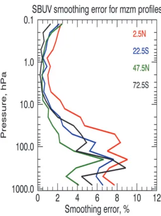
Figure 2 shows the SBUV smoothing error for mzm profiles as a function of altitude

5

for several latitude bands. Analysis of the SBUV retrieval algorithm and smoothing er-ror (Kramarova et al., 2013) demonstrates that the SBUV smoothing erer-ror is low (about 1–2 %) for individual layers between 25 and 1 hPa in mid- and high-latitudes (pole-ward of 20◦ latitude) and between 16 and 1 hPa in the tropics (20◦S–20◦N). In this vertical range SBUV ozone layer amounts can be directly compared to the

correspond-10

ing quantities obtained from the highly resolved measurements. Below and above this range the SBUV vertical resolution decreases and smoothing errors increase accord-ingly (up to 10–15 % in the troposphere). To reduce the smoothing error down to 1–2 %, we combine all layers below 25 hPa in the extratropics (or below 16 hPa in the tropics) down to 250 hPa (or down to the surface). In Sect. 4 we validate the SBUV ozone

15

amounts in the thick layers with the corresponding amounts obtained from Aura MLS (250–25 hPa and 250–16 hPa), ozonesonde (surface-30 hPa) and Umkehr (surface to 30 hPa) measurements.

2.4.3 Spatial and temporal coincident criteria

The spatial coincidence requirements vary depending on instrument. SBUV, UARS

20

and Aura MLS all have good spatial resolution with su_fficient sampling to produce rep-resentative monthly zonal mean values. Thus we do not use coincident profiles when comparing to MLS but simply compare mzm values directly. SAGE II data have com-paratively poor spatial/time coverage, so in this case we subset the SBUV dataset to match the SAGE space/time coverage. For each SAGE profile we find all SBUV

pro-25

(14)

ACPD

13, 2549–2597, 2013

Title Page

Tables Figures

◭ ◮

Back Close

Full Screen / Esc

Discussion

P

a

per

|

Dis

cussion

P

a

per

|

Discussion

P

a

per

|

Discussio

n

P

a

per

|

Then we construct monthly zonal means from the SAGE and sub-sampled SBUV for comparison. The same procedure is used when comparing SBUV to ground-based in-struments. We require at least five coincident profiles to calculate monthly means for ground-based microwave data and two profiles for lidar and Umkehr data. On average we typically have about 15 coincident microwave profiles, between 2 and 20 Umkehr

5

profiles and between 2 and 15 lidar profiles each month.

Appropriate coincidence criteria in both time and space are very important for vali-dation. We require measurements be taken within_±12 h for temporal coincidence for all instruments, except ground-based microwave spectrometers. However, above 1 hPa diurnal ozone variation plays a significant role (e.g. Connor et al., 1994; Haefele et al.,

10

2008), and time coincidence criteria should be stricter. For this reason we limit the ver-tical range of the validation to 1 hPa and below for all instruments except lidars, where we limit the upper range to 1.6 hPa due to the reduced number of lidar measurements above this altitude. Measurements from the ground-based microwave spectrometer at Mauna Loa are available at high time resolution so for these comparisons we

re-15

strict the time difference to_±1.5 h. The microwave instrument at Lauder also measures ozone profiles at high time resolution, but the number of profiles that satisfy to_±1.5 h coincident criteria is too low for statistical significance. Instead we calculate the daily average using all measurements between 09:00 a.m. and 05:00 p.m. local solar time to get a su_fficient number of profiles.

20

2.4.4 Bias, standard deviation and relative drift

The bias and standard deviation are calculated for each pair of instruments. The bias is the mean deviation of profiles measured by two different instruments:

b=

N

P

n=1

ˆ

Xsbuv−Xˆext

(15)

ACPD

13, 2549–2597, 2013

Title Page

Tables Figures

◭ ◮

Back Close

Full Screen / Esc

Discussion

P

a

per

|

Dis

cussion

P

a

per

|

Discussion

P

a

per

|

Discussio

n

P

a

per

|

where ˆXsbuv is the SBUV mzm ozone profile, ˆXext is the external mzm profile

(pro-file from the independent instrument) andN is the number of coincident profiles. To estimate the percent relative bias we normalize bias b by the SBUV a priori xa. The

corresponding standard deviation for the relative bias is estimated using:

σ2=

N

P

n=1

ˆ

Xsbuv−Xˆext−b 2

N (2)

5

We also compute the drift between the ozone time series from the instrument pairs. To estimate possible drifts for each SBUV instrument relative to various external measure-ments, we calculate monthly mean time series of seasonal anomalies by subtracting the seasonal cycle from each instrument independently. Then we compute the time se-ries of differences between the pair of deseasonalized anomalies and linearly regress

10

the difference time series at all altitudes. We deseasonalize anomalies to reduce per-sistence in the time series of residuals. This way we can assume that the residuals are random and normally distributed. Linear regression provides a simple way to estimate drift. The standard error for the slope of the linear regression is estimated using:

σslope(k)= q

d2₍_k₎ N−2 s

N

P

i=1

(p_i₋p)¯ 2

(3)

15

whered2(k)=PN

i=1(∆i(k)−a−bpi)2is the sum of the squared deviation between the seasonal anomaly differences ∆ and linear regression fits (a+bp) at layer k, N is the number of months, p is time and a and b are regression coefficients. Assuming a normal distribution, the 95 % confidence level of the slope is estimated as two times the standard error (Wilks, 2006).

(16)

ACPD

13, 2549–2597, 2013

Title Page

Tables Figures

◭ ◮

Back Close

Full Screen / Esc

Discussion

P

a

per

|

Dis

cussion

P

a

per

|

Discussion

P

a

per

|

Discussio

n

P

a

per

|

3 Results: mean biases and standard deviations

3.1 Relative to independent satellite measurements

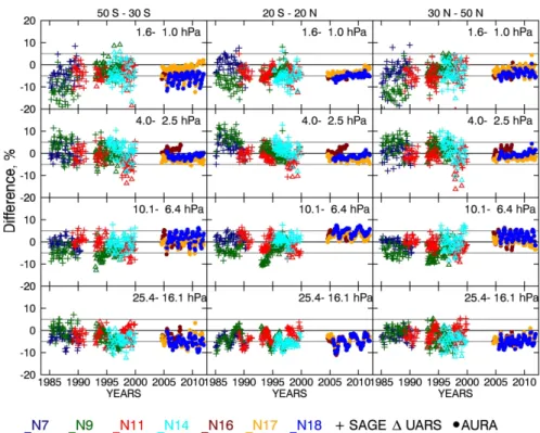
We validate SBUV mzm profiles relative to independent satellite measurements in the altitude range between 25 and 1 hPa. The time series of mzm differences for each SBUV instrument relative to independent satellite measurements for three latitude

5

zones (20◦_N–50◦_{N, 20}◦_S–20◦_{N and 20}◦_S–50◦_{S) and for di}

fferent layers are shown in Fig. 3. Various colors correspond to individual SBUV instruments. As we mentioned in Sect. 2.2.1, we consider here only SAGE II data from 1984 to 1999. During this time period SAGE II measurements overlap with four SBUV instruments: N7, N9, N11 and N14. UARS MLS overlaps with N9, N11 and N14 over its lifetime from 1991 to 1999;

10

Aura MLS overlaps with N16, N17 and N18 over the time period from October 2004 to 2011. The di_fferences between SBUV and independent instruments are mostly within ±10 %. Differences for N9, N11 and N14 relative to SAGE II and UARS closely fol-low each other. However, the range of differences is much narrower relative to Aura MLS compared to the earlier satellites. N16 demonstrates a drift starting from 2007

15

especially notable in the 4–2.5 hPa layer. This is the period when the N16 orbit was approaching the terminator.

It is important to notice a clear seasonal signature in the time series of differences relative to Aura MLS in the extratropics of both hemispheres. Differences relative to SAGE II and UARS MLS do not reveal a seasonal dependence, possibly because of

20

shorter overlaps with the SBUV instruments. In the tropical lower stratosphere (layer 25–16 hPa) the differences relative to all satellites show a clear signal of the Quasi Biennial Oscillations (QBO). Because of the low SBUV vertical resolution in the lower tropical stratosphere the SBUV algorithm is not capable of accurately retrieving the QBO signal in individual layers (Kramarova et al., 2013). Due to this limitation of the

25

(17)

ACPD

13, 2549–2597, 2013

Title Page

Tables Figures

◭ ◮

Back Close

Full Screen / Esc

Discussion

P

a

per

|

Dis

cussion

P

a

per

|

Discussion

P

a

per

|

Discussio

n

P

a

per

|

several layers from the surface (or from 250 hPa for Aura MLS comparisons) up to 16 hPa.

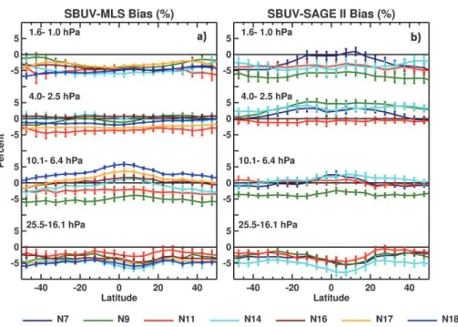
We calculate mean biases for each pair of instruments that have at least a 24-month overlap. Figure 4 shows mean biases for individual SBUV instruments relative to (a) MLS and (b) SAGE II mzm as a function of latitude in four layers between 25 hPa and

5

1 hPa. The left panel in Fig. 4 shows mean biases relative to UARS and Aura MLS. Biases for N9, N11 and N14 have been calculated relative to UARS MLS, while biases for N16, N17 and N18 have been calculated relative to Aura MLS. We do not calculate biases for N14 relative to Aura MLS, since the overlap time is less than 1 yr. Vertical bars on Fig. 4 indicate the standard error of the mean (σ/√N). The right panel in Fig. 4

10

demonstrates mean biases for four SBUV instruments (N7, N9, N11 and N14) relative to SAGE II.

Between 50◦S and 50◦N the mean biases are mostly within_±5 % for all SBUV in-struments. Between 25 and 10 hPa, below the ozone peak, all SBUV instruments un-derestimate ozone by about 3–5 % compared to the reference independent satellite

15

observations. We also found negative systematic biases in the layer between 1.6 and 1 hPa for all SBUV instruments, except for N7 which has almost zero o_ffset relative to SAGE II in the tropics.

Although for the most part SBUV instruments demonstrate consistent results, we note some features of individual instruments. N9 has larger negative o_ffsets in the

20

16–10 hPa and 10–6 hPa layers (more negative relative to UARS MLS compared with SAGE II) which is not consistent with the behavior of other SBUV instruments. N11 has negative biases relative to both UARS MLS and SAGE II throughout the vertical range. Again biases are more negative relative to UARS MLS than to SAGE II. The largest spread (_∼10 %) among the SBUV instruments is in the layer between 10 and 6 hPa,

25

where biases for the three recent SBUV instruments relative to Aura MLS are positive and biases for N9, N11 and N14 relative to UARS MLS are negative.

(18)

ACPD

13, 2549–2597, 2013

Title Page

Tables Figures

◭ ◮

Back Close

Full Screen / Esc

Discussion

P

a

per

|

Dis

cussion

P

a

per

|

Discussion

P

a

per

|

Discussio

n

P

a

per

|

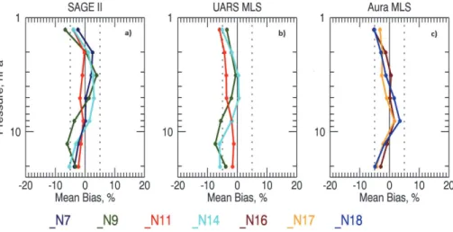
II, (b) UARS MLS and (c) Aura MLS. Again, the mean biases for the wide latitude band are mostly within the _±5 % range. Comparisons with UARS MLS and SAGE II show that the profile of mean biases for the ascending mode of N14 is very similar to the shape of the biases for N16, N17 and N18 relative to Aura MLS, with negative biases below 16 hPa and above 1.6 hPa and slightly positive or close to zero biases in

be-5

tween. The vertical shape of the biases for N7 relative to SAGE II is also very similar to that described above. N9 and N11 have slightly different shapes. N9 has large negative biases between 16 and 6 hPa, while N11 shows negative biases at all layers between 25 and 1 hPa. It is important to remember that N14, N16, N17 and N18 were calibrated against N17, while N7, N9 and N11 were calibrated against the Shuttle SBUV (Deland

10

et al., 2012). Thus similarity in shape of the mean biases for N7 and the four recent in-struments demonstrates that these inin-struments have common systematic errors which can be attributed to the SBUV retrieval algorithm itself rather than to features of the individual SBUV instruments. These results highlight the consistency among the indi-vidual SBUV instruments and add to the creditability of the SBUV merged data set for

15

long-term trend analysis.

The corresponding standard deviations (shown in Supplement, Fig. S1) for the mean biases relative to Aura MLS are less than 1.5 %, except for N16. In 2004 the N16 satel-lite started quickly drifting toward the terminator, and by the middle of 2007 the local equator crossing time passed 04:00 p.m. After mid-2007 the N16 di_fferences relative

20

to Aura MLS significantly increase. As a result the standard deviations are 2–2.5 %, while standard deviations computed for N16 over the period from October 2004 to July 2007 are the same order as for N17 and N18. For this reason we do not recommend using N16 measurements after mid-2007. Standard deviations for differences relative to UARS MLS and SAGE II are larger, varying within 1–5 %.

25

(19)

ACPD

13, 2549–2597, 2013

Title Page

Tables Figures

◭ ◮

Back Close

Full Screen / Esc

Discussion

P

a

per

|

Dis

cussion

P

a

per

|

Discussion

P

a

per

|

Discussio

n

P

a

per

|

amplitudes of seasonal variability are still mostly within 2–3 %, increasing up to 5–6 % in the 10–6 hPa layer. There is an approximately 6-month lag between southern and northern midlatitudes. We were not able to isolate clear seasonal structures from UARS MLS and SAGE comparisons. The amplitude of seasonal differences varies within_±2– 8 % and mostly less than 2σstandard deviations.

5

3.2 Relative to ground-based profile measurements

We validate SBUV profiles against three types of ground-based ozone profilers: mi-crowave spectrometers, lidars and Umkehr instruments. All instruments have different vertical resolutions and make measurements in various vertical ranges. We compare ozone amounts obtained from different instruments in vertical ranges where both

in-10

struments have sufficient information content and vertical resolution. For comparisons against microwave spectrometers, we consider ozone at 8 layers between 40 hPa and 1 hPa, and for lidar comparisons we validate ozone at 7 layers between 40 hPa and 1.6 hPa. We compare SBUV relative to Umkehr from the surface to 31 hPa, 31–16 hPa, 16 to 8 hPa, 8 to 4 hPa and 4 to 2 hPa. Comparisons for the layer between the surface

15

and 30 hPa are considered in Sect. 4.

3.2.1 Ground-based microwave

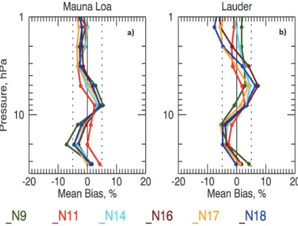
We validate SBUV ozone profiles against coincident microwave observations at Mauna Loa and Lauder. The vertical profiles of mean biases are shown in Fig. 6 for both microwave stations. Various colors correspond to different SBUV instruments. Biases

20

at both locations are negative between 25 and 10 hPa (up to₋7 %), which is consistent with the satellite comparisons. Between 10 and 4 hPa the biases are positive and flip sign above 2 hPa for all instruments except for N9 at Lauder. The main difference in the results for the two locations is the altitude where the biases switch sign from positive to negative. At Mauna Loa biases are positive above 4 hPa, while at Lauder the transition

25

(20)

ACPD

13, 2549–2597, 2013

Title Page

Tables Figures

◭ ◮

Back Close

Full Screen / Esc

Discussion

P

a

per

|

Dis

cussion

P

a

per

|

Discussion

P

a

per

|

Discussio

n

P

a

per

|

all SBUV instruments. However, we note that the shape of biases for N11 differs slightly from the other instruments, and N9 has larger biases. At Lauder we see a larger spread for individual SBUV instruments in upper levels. Above 2 hPa biases for N16, N17 and N18 are significantly negative and exceed 5 %, while the biases for N11 and N14 are less negative and close to zero. At the same time N9 has positive biases everywhere

5

above 6 hPa. The standard deviations of the differences at Mauna Loa average about 3 % and are almost independent of altitude. The standard deviations at Lauder are larger and vary from 3 to 5 %.

For microwave instruments we also calculate biases and standard deviations for in-dividual profiles without monthly averaging (results are not shown here). We found that

10

the value and shape of the biases remain the same, though the standard deviations increase approximately by a factor of 2.

3.2.2 SBUV vs. Lidars

We compared SBUV profiles with ground-based lidar observations at Mauna Loa, Table Mountain, Lauder and Haute Provence.

15

Figure 7 shows vertical profiles of SBUV mean biases relative to lidar measurements for all locations. Different colors correspond to different SBUV instruments. We can clearly see the consistency from station to station for the later instruments N16, 17 and 18. Biases are slightly negative between 25 and 10 hPa and positive between 10 and 4 hPa and then again switch sign above. However, at Lauder biases remain positive

20

above 4 hPa. Biases for the three recent SBUV instruments are mostly within a_±7 % range.

All earlier SBUV instruments demonstrate behavior that is not consistent from station to station or from one SBUV instrument to another. At Mauna Loa the vertical pattern of biases for N14 is very similar to that for N16, 17 and 18 with slightly less positive

25

(21)

ACPD

13, 2549–2597, 2013

Title Page

Tables Figures

◭ ◮

Back Close

Full Screen / Esc

Discussion

P

a

per

|

Dis

cussion

P

a

per

|

Discussion

P

a

per

|

Discussio

n

P

a

per

|

(N16–18) and positive up to+10 % for the four early instruments. Such inconsistency is most likely related to a major upgrade that was applied to the Table Mountain lidar in 2001 (http://tmf-lidar.jpl.nasa.gov/instruments/TMF strato DIAL.htm). At the Lauder station, biases above 10 hPa are negative for the earlier instruments and positive for the recent instruments, possibly due to fewer coincident profiles in this period. The

5

biases relative to lidar measurements at Haute Provence are very consistent and are mostly within 5 % for all SBUV instruments, except in the 2–1.6 hPa layer, where biases increase up to –10 %.

The standard deviations of the differences between monthly mean profiles are mostly within the 2–6 % range between 40 and 2 hPa. In the 2.5–1.6 hPa layer standard

de-10

viations increase to 10–12 % (see Supplement, Fig. S6). This again might be a result of the reduced lidar coverage at higher altitudes. The lowest standard deviations we found were for comparisons with Mauna Loa, where ozone variability is naturally low.

Comparisons with ground-based microwave spectrometers and lidars are consistent with the results we found above from the satellite comparisons. The vertical structure

15

of biases for N16, N17 and N18 is very robust. At some (but not all) stations the shape of biases for N14 is similar to the shape for the three recent instruments. N9 and N11 demonstrate different behavior which is inconsistent from station to station. It is impor-tant to note that the quality and frequency of ground-based measurements gradually increase over time. Thus larger uncertainties in 1990s can be partially attributed to the

20

lower quality of ground-based observations.

3.2.3 SBUV vs. Umkehr

Umkehr ground-based observations provide the longest record of ozone profiles, but the frequency of Umkehr measurements varies with location and over time. We select 6 Umkehr stations with relatively long time records and high quality of measurements

25

(22)

ACPD

13, 2549–2597, 2013

Title Page

Tables Figures

◭ ◮

Back Close

Full Screen / Esc

Discussion

P

a

per

|

Dis

cussion

P

a

per

|

Discussion

P

a

per

|

Discussio

n

P

a

per

|

60 to 90 degrees, thus in some locations (for example Belsk) Umkehr observations are not possible in winter.

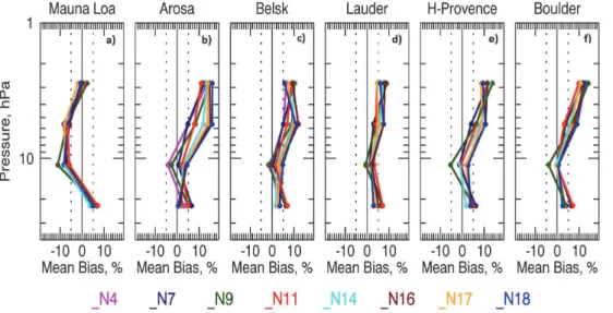
Figure 8 shows mean biases for individual SBUV instruments relative to Umkehr for all six locations. The vertical structures of biases are similar at all locations (except Mauna Loa) with positive biases between 8 and 2 hPa and between 30–16 hPa.

Be-5

tween 16 and 8 hPa biases tend to be closer to zero. Similar results were shown by Nair et al. (2011), where authors noticed low Umkehr ozone values at Haute Provence relative to lidar observations at the same location. At Mauna Loa the vertical structure of biases is similar to that described above, except biases are negative between 8– 4 hPa. The similar structure of biases at all locations points on the systematic error in

10

the Umkehr retrievals, causing Umkehr instruments underestimate ozone amounts in the stratosphere.

At Mauna Loa, Belsk, Lauder, Haute Provence and Boulder the vertical structures of the biases for all SBUV instruments are very similar. At Arosa, the last four instruments demonstrate similar behavior, while N4, N7, N9 and N11 show less positive biases in

15

layers between 16 and 4 hPa. The standard deviations of monthly mean biases vary from 2 to 6 %, with larger standard deviations at Belsk (up to 10–12 %) for N17 and N18.

The Umkehr technique measures the entire profile, so we also compare total col-umn ozone amounts with those obtained from SBUV instruments. Biases are mostly

20

positive and vary from 1–3 % with corresponding standard deviations of about 4 %. Labow et al. (2013) compared SBUV v8.6 total ozone against ground-based Dobson and Brewer observations and found differences within_±1 %.

We also calculated seasonal biases for comparisons with ground-based stations (re-sults are shown in the Supplement, Figs. S11–S13). Similarly to satellite comparisons,

25

(23)

ACPD

13, 2549–2597, 2013

Title Page

Tables Figures

◭ ◮

Back Close

Full Screen / Esc

Discussion

P

a

per

|

Dis

cussion

P

a

per

|

Discussion

P

a

per

|

Discussio

n

P

a

per

|

range of standard deviations. We find clear seasonal structures relative to the instru-ments at Lauder (microwave spectrometer, lidar and Umkehr). Particularly, we isolate a robust seasonal pattern in the 10–6 hPa layer with negative biases in winter and pos-itive biases in summer. The seasonal pattern at Lauder in this layer is consistent with Aura MLS comparisons. However, at other layers the seasonal pattern is not consistent

5

from one ground-based instrument to another and not consistent with Aura MLS. The cause of the larger seasonal biases between SBUV measurements and ground-based observations at Lauder is not clear.

4 Results: validation of partial ozone columns in the lower stratosphere and troposphere

10

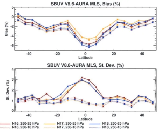
In order to get around the issue of di_ffering vertical resolution, we compare SBUV ozone partial columns in the lower stratosphere and troposphere with corresponding values obtained from Aura MLS. Figure 9 shows the mean biases and standard devi-ations as a function of latitude for two recommended layer combindevi-ations: 250–25 hPa and 250–16 hPa. The biases for the 250–25 hPa layer are 0–2 % outside of the tropics.

15

In the narrow tropical zone between 20◦S and 20◦N biases increase to₋6 %. The bi-ases are slightly more negative for the 250–16 hPa layer outside of the tropics, but the latitudinal structures are similar to those described above (dotted lines on Fig. 9). Pre-viously Froidevaux et al. (2008) also detected positive biases in the troposphere/lower stratosphere for Aura MLS v.2.2, meaning that Aura MLS slightly overestimate ozone

20

concentration here.

The corresponding standard deviations for the 250–25 hPa layer vary within 1–2 % outside the tropics and increase to 3–4 % in the tropics. However, the standard de-viations are reduced to 1 % over the tropics for the broader 250–16 hPa layer. This example demonstrates the increase in the precision of SBUV measurements in the

25

(24)

ACPD

13, 2549–2597, 2013

Title Page

Tables Figures

◭ ◮

Back Close

Full Screen / Esc

Discussion

P

a

per

|

Dis

cussion

P

a

per

|

Discussion

P

a

per

|

Discussio

n

P

a

per

|

between the SBUV and MLS measurements at individual layers in the lower tropical stratosphere varies from 3 to 10 % (results not shown here).

In addition, we compare partial ozone columns between the surface and 30 hPa against corresponding amounts obtained from the ensemble of 4 northern mid-latitude Umkehr instruments (see Fig. 10). The color lines on this plot show the time series of

5

differences for individual SBUV instruments, while the thick black line shows the 12-month moving average. The number of stations changes each 12-month, and we require observations from at least two stations. The biases are mostly within_±5 %. The mean biases are very close to zero between 1995 and 2011. In the late 1980s-early 1990s mean biases are negative with amplitudes of₋2 to₋3 %.

10

We also validate the SBUV partial ozone columns between the surface and 30 hPa with the corresponding values obtained from the ensemble of 4 ozonesonde stations at Boulder (40◦S), Hohenpeissenberg (48◦N), Lindenberg (52◦N) and Payerne (47◦N). These ozonesonde stations were selected for their proximity to the northern midlati-tude Umkehr stations. Figure 11 shows time series of differences between SBUV and

15

ozonesonde measurements. The thick black lines show 12-month moving averages. Biases are mostly positive with a mean bias of about 2 %.

Results shown in Fig. 9–11 demonstrate that despite the limited SBUV vertical res-olution in the lower stratosphere and troposphere, the partial ozone columns obtained from SBUV instruments agree within_±5 % with the corresponding values observed by

20

independent satellite and ground-based instruments.

5 Results: drifts

We estimate possible drifts in the SBUV time series relative to independent ground-based and satellite measurements as described in Sect. 2.4.4. However, the short overlap periods between SBUV and reference instruments, degradation of satellite

in-25

(25)

ACPD

13, 2549–2597, 2013

Title Page

Tables Figures

◭ ◮

Back Close

Full Screen / Esc

Discussion

P

a

per

|

Dis

cussion

P

a

per

|

Discussion

P

a

per

|

Discussio

n

P

a

per

|

measurements on both the ascending and descending modes of their orbit. DeLand et al. (2012) show that often instrument behavior appears to change after crossing the terminator. Thus we estimate drifts for ascending and descending modes separately.

5.1 Drifts relative to satellite instruments

For drift calculations we require at least a 24-month overlap between two time series.

5

Figure 12 shows drifts for individual SBUV instruments relative to independent satellite measurements as functions of latitude. Vertical bars indicate two times the standard error for the slope which corresponds to the 95 % confidence level. Various colors correspond to individual SBUV instruments. We estimate drifts relative to Aura MLS for the three recent instruments N16, N17 and N18. The N16 record starts drifting

10

notably after the mid-2007 (see Fig. 3) when the instrument equatorial crossing time passes 04:00 p.m. Thus here we show drifts for N16 only up to mid-2007. We evaluate drifts for N9 descending and N14 ascending relative to both SAGE II and UARS MLS. Overlapping time periods for N11 ascending and descending mode with UARS MLS are less than 24 months and drifts were not computed. Drifts for N7, N9 ascending,

15

N11 ascending and descending are estimated relative to SAGE II.

Drifts relative to the MLS instruments are mostly within_±1 % yr−1, except for N9 de-scending (Fig. 12a). N17 has the smallest drifts (mostly less than_±0.3 % yr−1_{) among}

all SBUV instruments. N18 also has small drifts (less than 0.5 % yr−1) everywhere, ex-cept in layer 25–16 hPa where drifts over the tropics increase up to 0.5–0.9 % yr−1.

20

Drifts are slightly larger for N16 (up to 1 % yr−1_{) due to the shorter overlap period with}

Aura MLS observations (October 2004–June 2007). We estimated drift for the whole N16 record (results are not shown here) and found drifts varying from₋2.5 % yr−1 to 2 % yr−1_{. N9 descending has larger drifts in the tropics up to 2 % yr}−1_{in the 10–6.4 hPa}

layer and more than₋1 % yr−1drifts in the 25–16 hPa layer.

25

(26)

ACPD

13, 2549–2597, 2013

Title Page

Tables Figures

◭ ◮

Back Close

Full Screen / Esc

Discussion

P

a

per

|

Dis

cussion

P

a

per

|

Discussion

P

a

per

|

Discussio

n

P

a

per

|

drifts less than 1 % yr−1everywhere except the 1.6–1 hPa layer where drifts slightly ex-ceed_±1 % yr−1. N7 has small but significant negative drifts relative to SAGE II in both northern and southern midlatitudes between 16 and 6 hPa and positive drifts above 2.5 hPa. In the tropics the N7 drifts are significant and positive above 6 hPa. Drifts for N9 ascending are larger over the tropics, with ascending mode drifts of+2–3 % yr−1

5

between 25 and 16 hPa and₋3 % yr−1_{between 6 and 2.5 hPa (this layer is not shown}

in Fig. 12). Drifts in the descending mode of N9 measurements are up to₋1 % yr−1 at 25–16 hPa, +2 % yr−1 between 10 and 6 hPa and about +1 % yr−1 above 1.6 hPa for all latitudes. We estimate drifts for the descending mode of N9 relative to both SAGE II and UARS MLS and find similar results. The drifts for N11 ascending are mostly less

10

than 0.5 % yr−1 through the considered altitude range. However, we found large and significant drifts during the descending portion of N11, with the largest drifts over the tropics. N11 descending drifts vary from up to₋1.5 % yr−1 between 25 and 10 hPa to

+2 % yr−1 between 6 and 1.6 hPa. We also found statistically significant drifts in the N14 ascending mode measurements in all latitude bands relative to both SAGE II and

15

UARS MLS. N14 has larger drifts relative to SAGE than relative to UARS MLS. The N14 drifts relative to SAGE II exceed₋1 % yr−1in the layer 4–2.5 hPa.

Figure 13 shows drifts for SBUV instruments relative to independent satellite mea-surements as a function of altitude for the wide latitudinal band 50◦S–50◦N. The drifts for N7 and N11 ascending are small and less than 0.6 % yr−1 (Fig. 13a, b), and the

20

N11 ascending drifts are mostly insignificant. The drifts of the three recent SBUV in-struments relative to Aura MLS (Fig. 13d) are also less than 0.5 % yr−1 and mostly insignificant. Both portions of N9, N11 descending and N14 ascending have larger drifts that exceed_±1 % yr−1_{. Drift estimations relative to UARS and SAGE for N9}

de-scending and N14 ade-scending are consistent. The vertical structure of the N14 drift is

25

(27)

ACPD

13, 2549–2597, 2013

Title Page

Tables Figures

◭ ◮

Back Close

Full Screen / Esc

Discussion

P

a

per

|

Dis

cussion

P

a

per

|

Discussion

P

a

per

|

Discussio

n

P

a

per

|

5.2 Drifts relative to ground-based instruments

Our analysis demonstrates that records from some stations have obvious time-dependent changes (see Supplement, Figs. S2–S4). Thus we choose only instruments that show no signs of such temporal changes to estimate drifts. We evaluate SBUV drifts relative to lidars at Haute Provence, Mauna Loa and Lauder. We exclude Table

5

Mountain due to changes above 4 hPa that occurred after the repair in 2001. We use records from four Umkehr stations: Arosa, Lauder, Haute Provence and Boulder; we exclude Mauna Loa Umkehr due to significant stray light problems and Belsk due to missing measurements during winter. We relax the overlap criteria to 18 months for the ascending and descending portions of N9 and N11 to account for shorter overlap

10

periods with ground-based data.

Figure 14 shows vertical profiles of the mean drifts for each SBUV instrument relative to each type of ozone profiler. Drifts relative to all ground-based instruments are shown in the Supplement (Figs. S15–S17). The top panel shows the drifts over the time period 2000–2011 and the bottom panel shows drifts over the time period 1985–1999. As

15

before the three recent instruments have smaller drifts. In particularly N17 has proved to be a stable instrument with drifts mostly within_±0.2 % yr−1. Slightly larger drifts for N18 are most likely due to the shorter overlap periods. Generally, drifts for N16 and N18 are within_±0.5 % yr−1_{and never exceed}

±1 % yr−1. Drifts in the N11 ascending mode and N7 data relative to ground-based Umkehr observations are less than _±1 % yr−1.

20

We estimate drift in N4 relative to measurements from the Umkehr instrument at Arosa (see Supplement, Fig. S17) and find that drifts are statistically insignificant. However, this is not an independent measure because the N4 radiance calibration was made relative to Arosa measurements (Bhartia et al., 2012). We detected rather large drifts (more than_±1 % yr−1) for ascending and descending modes of N9 and N14 and for

25