www.atmos-meas-tech.net/8/4487/2015/ doi:10.5194/amt-8-4487-2015
© Author(s) 2015. CC Attribution 3.0 License.
Spatial mapping of ground-based observations of total ozone
K.-L. Chang1, S. Guillas1, and V. E. Fioletov2
1Department of Statistical Science, University College London, London, UK 2Environment Canada, Toronto, Ontario, Canada
Correspondence to:K.-L. Chang (ucakkac@ucl.ac.uk)
Received: 26 January 2015 – Published in Atmos. Meas. Tech. Discuss.: 22 April 2015 Revised: 29 September 2015 – Accepted: 7 October 2015 – Published: 23 October 2015
Abstract. Total column ozone variations estimated using ground-based stations provide important independent source of information in addition to satellite-based estimates. This estimation has been vigorously challenged by data inhomo-geneity in time and by the irregularity of the spatial distri-bution of stations, as well as by interruptions in observation records. Furthermore, some stations have calibration issues and thus observations may drift. In this paper we compare the spatial interpolation of ozone levels using the novel stochas-tic partial differential equation (SPDE) approach with the covariance-based kriging. We show how these new spatial predictions are more accurate, less uncertain and more ro-bust. We construct long-term zonal means to investigate the robustness against the absence of measurements at some sta-tions as well as instruments drifts. We conclude that time se-ries analyzes can benefit from the SPDE approach compared to the covariance-based kriging when stations are missing, but the positive impact of the technique is less pronounced in the case of drifts.
1 Introduction
The ground-based total column ozone data set is based on Dobson and Brewer spectrophotometer and filter ozonometer observations available from the World Ozone and UV Data Centre (WOUDC) (http://www.woudc.org/). Large longitu-dinal inhomogeneities in the global ozone distribution and limited spatial coverage of the ground-based network make it difficult to estimate zonal and global total ozone values from station observations directly (Fioletov et al., 2002). The Total Column Ozone (TCO) data set is comprised of the ozone ob-servations from the set of ground-based stations worldwide. Most of those stations are located on land in the Northern
Hemisphere, and relatively few stations are over the Southern Hemisphere and oceans. Therefore the spatial distribution of ground-based stations is highly irregular. In addition, dura-tions of operadura-tions for each station are different. One of the major difficulties in assessing long-term global total ozone variations is thus data inhomogeneity. Indeed recalibration of ground-based instruments, or interruptions in observation records result in data sets which may have systematic errors that change with time (Fioletov et al., 2002, 2008).
The TCO data set and corresponding satellite measure-ments have also been widely discussed in the statistics lit-erature. Some authors have noticed space–time asymmetry in ozone data (Stein, 2005, 2007; Jun and Stein, 2007, 2008). The other important feature of TCO data is that the spatial dependence of ozone distributions varies strongly with lati-tude and weakly with longilati-tude, so that homogeneous mod-els (invariant to all rotations) are clearly unsuitable (Stein, 2007). This is why Jun and Stein (2007) assume that the spa-tial process driving the TCO data is an axially symmetric process whose first two moments are invariant to rotations about the Earth’s axis, and constructed space–time covari-ance functions on the sphere×time that are weakly station-ary with respect to longitude and time for fixed values of latitude. Jun and Stein (2008) further used linear combina-tions of Legendre polynomials to represent the coefficients of partial differential operators in the covariance functions. These covariance functions produce covariance matrices that are neither of low rank nor sparse for irregularly distributed observations, as it is the case with ground-based stations. Hence, likelihood calculations can thus be difficult in that situation, and we will not follow this approach.
evalu-values and compare them with zonal means calculated from ground-based data and available from the WOUDC (Bojkov and Fioletov, 1995; Fioletov et al., 2002).
Section 2 gives a brief introduction to the theoretical framework of the SPDE technique, a basic description of the covariance-based kriging and related model selection and di-agnostic techniques. Section 3 describes the spatial analy-sis using TCO data from WOUDC on a monthly, seasonal and annual basis. Furthermore, the estimated results of SPDE and covariance-based kriging are compared with the Total Ozone Mapping Spectrometer (TOMS) satellite data to ex-amine which method yields approximations closer to satel-lite data. Finally, the long-term zonal mean trends enable us to conduct a sensitivity analysis by removing stations at random and by introducing long-term drifts at some ground-based stations.
2 Methods
Our main problem is to estimate ozone values at places where it is not observed. Models in spatial statistics that enable this task are usually specified through the covariance function of the latent field. Indeed, in order to assess uncertainties in the spatial interpolation with global coverage, we cannot build models only for the discretely located observations, we need to build an approximation of the entire underlying stochastic process defined on the sphere. We consider statistical mod-els for which the unknown functions are assumed to be re-alizations of a Gaussian random spatial process. The stan-dard fitting approach, covariance-based kriging, spatially in-terpolates values as linear combinations of the original ob-servations, and this constitutes the spatial predictor. Not only large data sets can be computationally demanding for a krig-ing predictor but covariance-based models also struggle to take into consideration in general nonstationarity (i.e., when physical spatial correlations are different across regions) due to the fixed underlying covariance structure. Recently, a dif-ferent computational approach (for identical underlying spa-tial covariance models) was introduced by Lindgren et al. (2011), in which random fields are expressed as a weak so-lution to an SPDE, with explicit links between the param-eters of the SPDE and the covariance structure. This ap-proach can deal with large spatial data sets and naturally ac-count for nonstationarity. We review below some of the re-cent development on the covariance structure modeling on
ance functions, both in terms of accuracy and quantification of uncertainty. The shape parameterν, scale parameterκand the marginal precisionτ2parameterize it:
C(h)= 2
1−ν
(4π )d/2Ŵ(ν+d/2)κ2ντ2(κkhk) νK
ν(κkhk), (1)
whereh∈Rd denotes the difference between any two loca-tionssands′:h=s−s′, andKν is a modified Bessel
func-tion of the second kind of orderν>0. 2.1 SPDE approach
LetX(s)be the latent field of ozone measurementsY (s) un-der observation errorsǫ(s). Lindgren et al. (2011) use the fact that a random processX(s)onRdwith a Matérn covariance
function (Eq. 1) is the stationary solution to the SPDE:
(κ2−1)α/2τ X(s)=W(s), (2)
whereW(s)is Gaussian white noise, and1is the Laplace operator. The regularity (or smoothness) parameterν essen-tially determines the order of differentiability of the fields. The link between the Matérn covariance (Eq. 1) and the SPDE formulation (Eq. 2) is given byα=ν+d/2, which makes explicit the relationship between dimension and reg-ularity for fixedα. Unlike the covariance-based model, the SPDE approach can be easily manipulated on manifolds. On more general manifolds thanRd, the direct Matérn represen-tation is not easy to implement, but the SPDE formulation provides a natural generalization, and theν parameter will keep its meaning as the quantitative measure of regularity. Instead of defining Matérn fields by the covariance function on these manifolds, Lindgren et al. (2011) used the solution of the SPDE as a definition, and it is much easier and flexi-ble to do so. This definition is valid not only onRdbut also on general smooth manifolds, such as the sphere. The SPDE approach allowsκandτ to vary with location:
(κ2(s)−1)α/2τ (s)X(s)=W(s), (3)
SPDEs on triangulations, INLA provides good approxima-tions of posterior densities at a fraction of the cost of Markov chain Monte Carlo. Note that for models with Gaussian data, the calculated densities are for practical purposes exact. 2.2 Covariance-based approach
For locations on spherical domain,si=(Li,li), letY (si)
de-note the ozone measured at stationi. Then the kriging repre-sentation can be assumed additive with a polynomial model for the spatial trend (universal kriging):
Y (si)=P (si)+Z(si)+ei,
whereP is a polynomial which is the fixed part of the model,
Z is a zero mean, Gaussian stochastic process with an un-known covariance functionKandei are i.i.d. normal errors.
The estimated latent field is then the best linear unbiased es-timator (BLUE) ofP (s)+Z(s)given the observed data. Note that the Gaussian process in the spatial model,Z(s), can be defined as a realization of the processX(s)from the previous section.
For the covariance-based approach, the hurdle that we are facing is that we have to define a valid (but flexible enough) covariance model and, furthermore, compared to data on the plane, we must employ a distance on the sphere. Two dis-tances are commonly considered. The chordal distance be-tween the two points (L1,l1)and(L2,l2)on the sphere is
given by
ch(L1,L2,l1−l2)=
2r
sin2
L
1−L2
2
+cosL1cosL2sin2
l
1−l2
2
1/2
,
where r denotes the Earth’s radius. The more physically intuitive great circle distance between the two locations is gc(L1,L2,l1−l2)=2rarcsin{ch(L1,L2,l1−l2)}. However,
Gneiting (2013) pointed out that using the great circle dis-tance in the original Matérn covariance function (Eq. 1) would not work, as it may not yield a valid positive defi-nite covariance function. Therefore in this study we use the chordal distance for covariance-based kriging. The main ad-vantage of using the chordal distance is that it is well de-fined on spherical domains, as it restricts positive definite covariance functions onR3toS2(Jun and Stein, 2007). For the ozone data, we specify the Matérn covariance function defined in Eq. (1) in the covariance-based approach in or-der to compare the performance with the SPDE approach for exactly the same covariance function, whereas the model parameters are optimized according to different techniques. The relevant model diagnostic and selection criteria are de-scribed in Appendix B. Note that the smoothness parameter
ν is allowed to be selected in the covariance-based kriging, whereas we fix it atν=1 in the SPDE approach.
3 Mapping accuracy
In this section, we produce statistical estimates of monthly ozone maps, using TCO data from WOUDC. We consider TCO data in January 2000 as an illustration, which contain 150 ground-based ozone observations around the world. All ozone values in this article are in Dobson units (DU). We first choose the model setups for both SPDE and covariance-based approaches below.
With the SPDE approach, as the smoothness parameter
ν is defined through the relationshipα=ν+d/2 (see Ap-pendix A1), we only need to choose the basis expansion or-der to representκandτ. To choose the best maximal order of the spherical harmonic basis, we fitted models with different maximal orders of spherical harmonics for the expansions of
κandτ in order to estimate them thereafter (the default for-mulation in the R-INLA package). The best fitted model is for a spherical harmonics basis with maximal order 3 since it yielded the lowest generalized cross-validation (GCV) stan-dard deviation (SD) computed in Eq. (B2), which yields a to-tal of nine parameters to be estimated (four parameters for the expansions ofκ andτ and one parameter for the variance). For the covariance-based approach, we need to choose the smoothness parameter in the Matérn covariance function be-fore estimating the univariate quantitiesκ andτ2. The same
σGCV criterion is used to evaluate the model performance.
We fit a wide range of values for the smoothing parameter, andν=20 minimizes theσGCVfor these ozone data.
To compare the performance of the SPDE approach with the covariance-based kriging, the same σGCV criterion is
used as it balances well predictive power vs. overfitting across methods. We first estimate the optimized model pa-rameters, i.e., κ and τ in a SPDE and ν in a covariance-based model, by the same generalized cross-validation cri-terion (with different computational methods, the estimated method for the chordal distance covariance model is max-imum likelihood estimates), then compare the uncertainty of spatial estimation over the surface. For the prior spec-ifications of the SPDE approach,κ andτ follow log nor-mal priors by default: precision (theta.prior.prec) = 0.1, me-dian for τ (prior.variance.nominal) = 1 and median for κ
(prior.range.nominal) depends on the mesh. We use a regres-sion basis of spherical harmonics for both of these parame-ters; therefore by default the coefficients follow the log nor-mal priors. We do not change the R-INLA default prior set-tings throughout the analysis.
(a) SPDE mean (b) SPDE SD
(c) CBK mean (d) CBK SD
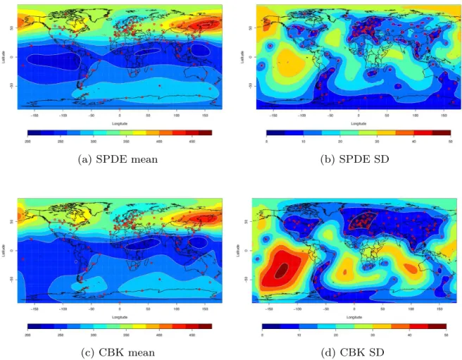
Figure 1.Surface predicted ozone (DU) mean and SD for SPDE (strategy D) and CBK (strategy B) from January 2000. The red points indicate the locations of stations.
Table 1.Specifications of the different strategies in the spatial esti-mations.
Strategy Descriptions
A A covariance-based model withν=1 B A covariance-based model withν=20
C An SPDE-based model with stationary covariance parameters (i.e.,κandτare unknown constants) D An SPDE-based model with space-varying
covariance parameters
We now compare the results estimated by four strategies described in Table 1. We start an illustration to 6 years of monthly observations. The results of the analysis of ozone data averaged from 2000 to 2005 are shown in Table 2. The averaged number of available stations is denoted byn, and the residual sum of square (RSS) indicates residuals sum of square, which is defined in Eq. (B1). The SPDE approach (strategies C and D) provides a better fit than the covariance-based kriging (strategies A and B) for all months. The effec-tive degree of freedomneff is higher in the SPDE approach
as it is more complex than covariance-based kriging. Higher
effective degrees of freedom means smaller values in the
σGCVdenominator (n−neff) and thus higher values forσGCV
to account for overparametrization. Nevertheless,σGCV
val-ues for the SPDE approach are still all much lower than for covariance-based kriging in all cases. This means that the RSS in the SPDE approach is drastically smaller than the RSS for covariance-based kriging. Thus the SPDE approach supplies a much better fit to the true ozone observation. Note that the covariance-based model is computing a weighted av-erage of the neighborhood values around the location, while the SPDE model is constructed through a triangular mesh. The mesh can be more adaptive and flexible to irregularly distributed observations. In addition, with spatially varyingκ
andτ, the table indicates that the results could be improved further by applying a nonstationary extension.
Table 2.Comparison of the generalized cross-validation error (σGCV) and the residual sum of square (RSS) for different strategies averaged of 2000–2005 by month. Statistical summaries for Northern Hemisphere (NH), tropics and Southern Hemisphere (SH).
Global statistics Jan Feb Mar Apr May Jun Jul Aug Sep Oct Nov Dec
Number of obs. 135.33 144.33 146.17 146.00 142.50 143.33 143.00 145.33 146.00 142.67 140.17 129.50
A neff 16.00 20.92 26.84 17.50 28.23 22.96 11.20 31.67 53.11 60.29 30.09 19.67
σGCV 16.62 17.51 14.97 13.29 10.83 10.23 10.35 11.20 13.19 12.67 17.17 15.58 RSS 34 584 39 599 28 017 23 405 13 884 13 333 14 300 14 688 19 312 13 379 34 470 28 416
B neff 16.89 25.69 30.51 19.57 24.14 15.46 14.39 29.63 36.93 38.24 28.86 20.67
σGCV 15.10 14.05 12.11 12.45 10.33 10.54 9.87 9.75 9.68 9.53 12.35 12.71
RSS 28 535 25 611 18 323 20 711 13 258 14 770 12 637 11 479 10 654 9645 17 550 19 129
C neff 70.33 60.76 81.23 59.31 64.87 76.23 48.70 54.63 65.13 75.41 72.09 51.12
σGCV 11.89 10.33 8.39 9.24 6.06 6.77 7.78 7.61 6.71 6.15 9.45 8.91
RSS 12 263 10 085 5394 9600 3428 4283 6224 6351 4400 2600 6924 6897
D neff 67.75 59.12 73.08 61.01 72.01 84.44 60.14 64.71 73.67 75.21 72.00 62.97
σGCV 8.60 9.90 7.90 9.18 6.27 6.80 7.22 6.85 6.62 5.75 8.84 7.90
RSS 6148 9431 5312 8664 3359 3865 4326 4845 4179 2285 5924 4805
RSS by region Jan Feb Mar Apr May Jun Jul Aug Sep Oct Nov Dec
Number of obs. 89.50 98.50 101.67 104.00 102.50 103.83 103.00 103.00 102.67 98.50 95.50 84.67
NH A 29 531 34 011 23 399 17 207 9981 9692 8844 6933 6118 4159 16 117 22 115
B 26 035 22 234 15 507 16 144 10 498 11 288 8435 7238 7179 6748 13 035 16 690
C 11 543 9248 4895 8002 2932 3415 4467 4519 3490 2011 5649 6082
D 4119 7240 4183 6696 2880 3328 3384 3903 3709 1914 5104 3301
Number of obs. 27.83 27.33 26.33 26.33 26.50 26.67 27.33 27.33 26.83 26.67 27.00 27.17
Tropics A 3706 3666 3461 4082 1758 1671 2766 2253 2898 2286 4123 3008
B 1778 2182 2120 2988 1254 1632 2264 1228 957 1042 1360 1411
C 413 489 367 1095 219 280 830 489 238 192 397 454
D 1148 1438 688 1142 331 368 646 441 171 120 309 990
Number of obs. 18.00 18.50 18.17 15.67 13.50 12.83 12.67 15.00 16.50 17.50 17.67 17.67
SH A 1347 1922 1157 2116 2144 19 670 2689 5502 10 296 6933 14 230 3293
B 722 1195 696 1580 1505 1850 1938 3012 2518 1855 3155 1028
C 306 348 162 504 277 588 927 1343 672 397 878 361
D 882 754 442 827 148 169 295 501 299 251 510 515
regions. Lower estimation errors can be found in August– October and higher errors occur in December–February.
Figure 1 shows the predicted mean and SD ozone maps by strategies B and D on January 2000. The spatial distribu-tions of ozone means are similar for SPDE and covariance-based kriging in the Northern Hemisphere, but there are dif-ferences in the Southern Hemisphere. These difdif-ferences arise from the asymmetry of available stations in the two hemi-spheres. The spatial distributions of the SD present similar general patterns for the two techniques. The uncertainties are higher where with fewer stations are available, see the large uncertainty distribution over the South Pacific Ocean. SDs of SPDE predictions are much smaller than the SDs of the covariance-based kriging predictions, especially where fewer observations are available (e.g., mid-Atlantic and South Pa-cific), but are larger near the North Pole; this may be due to covariance-based kriging underestimating its own uncer-tainty.
3.1 Seasonal and annual effects
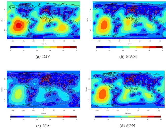
Seasonal ozone data are obtained by averaging the cor-responding monthly data (but all months of every season must be available to create such seasonal averages). Ta-ble 3 shows the seasonal results for different strategies over the years 2000–2005. Their respective highest errors are in December–January–February (DJF) for strategies A, B and C and in June–July–August (JJA) for strategy D. The re-sults are hardly different in March–April–May (MAM) and September–October–November (SON) for strategies C and D, while a significant improvement can be achieved in DJF by applying a nonstationary SPDE model. Moreover, the val-ues ofσGCVand RSS from this seasonal analysis are smaller
(a) DJF (b) MAM
(c) JJA (d) SON
Figure 2.Surface predicted ozone (DU) mean from SPDE approach (strategy D) by season from 2000.
Table 3. Generalized cross-validation error (σGCV) and residual sum of square (RSS) for different strategies averaged over 2000– 2005 by season.
Season DJF MAM JJA SON Average n 117.17 132.83 132.17 130.67 128.21 A neff 13.45 21.66 13.01 52.06 25.04 σGCV 11.95 9.96 8.65 11.23 10.45 RSS 16 194 11 513 8987 10 178 11 718
B neff 18.73 20.68 11.53 32.77 20.93 σGCV 9.47 9.20 8.39 8.19 8.81 RSS 10 274 9990 8526 6783 8893
C neff 48.10 60.41 50.25 75.00 58.44 σGCV 7.72 5.86 6.41 6.47 6.46
RSS 4661 3120 4140 2272 3548
D neff 52.82 64.43 58.06 77.07 63.09 σGCV 6.55 6.00 6.13 5.82 6.12
RSS 2695 3074 3609 2210 2897
SD, respectively. The maps for SD again reveal the higher estimated error in regions without stations.
The annual ozone data are obtained by creating an an-nual average, which also means that stations with record
in-terruptions are not used. Therefore fewer stations are avail-able for this exercise. To see the improvement of the annual-based analysis over seasonally and monthly analyses, Ta-ble 4 shows the annual averaged results by month and sea-sonally, and the results directly obtained by doing the analy-sis on the annual mean. Although there are fewer stations in annual-based and seasonal-based data than in monthly data, the errors are lower than for monthly data over the years for all strategies and the results directly obtained from annual means yield even lower RSS andσGCVthan the results
aver-aged by seasons due to smooth variation. 3.2 Comparison with satellite data
In this section, we assess the match between satellite ob-servations and spatial predictions based on ground-level stations. The TOMS data on monthly averages are ob-tained from the NASA website (http://ozoneaq.gsfc.nasa. gov/), where we collected the Earth Probe (25 July 1996– 31 December 2005) satellite data with grid 1◦×1.25◦. We calculate the differences over all grid cells and summarize it by the root mean square error (RMSE). Let yˆi be the
(a) DJF (b) MAM
(c) JJA (d) SON
Figure 3.Surface predicted ozone (DU) standard deviation from SPDE approach (strategy D) by season from 2000.
(normalized) RMSE is given by
RMSE= s
Pn
i=1 yˆi−yis
2
n ,
wheren=180×288 is total number of grid cells. However, satellite data are unavailable over high latitudes in DJF and MAM and over low latitudes in JJA and SON. Therefore we restrict the calculations of RMSEs between 60◦S and 60◦N. From this stage we only compare the results between a nonstationary SPDE-based model and a covariance-based model with ν=20. Monthly comparisons over 2000–2005 are shown in Table 5. Ozone surfaces predicted by the SPDE approach are closer to the satellite data than the predictions from covariance-based kriging over all months. The high-est improvement of SPDE over covariance-based kriging is 77.15 % in September and the lowest is 33.60 % in May. Also, in contrast with relatively unstable monthly predictions by covariance-based kriging, SPDE shows more consistency in predictions of monthly ozone variation.
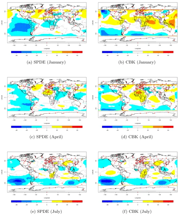
Figures 4 and 5 map the differences of surface predic-tions of covariance-based and SPDE methods with respect to satellite data over 60◦S–60◦N on January, April, July and October 2000. The differences in October turn out to
be much larger than in other months, and therefore a dif-ferent scale is used. These maps indicate the overestima-tion (red) and underestimaoverestima-tion (blue) with respect to satel-lite data. Similar patterns in deviations are revealed for both techniques, but SPDE displays less magnitude in the devia-tions than covariance-based kriging. One noticeable feature is that the pattern of deviation from satellite data is strongly related to the distribution of ground-based stations: for in-stance, the covariance-based kriging predicted surfaces tend to underestimate the values over the South Pacific Ocean, where few stations are available. The surface predictions by SPDE achieve a clear improvement in predictions compared to covariance-based kriging over areas with less stations, es-pecially in January and October.
es-(a) SPDE (January) (b) CBK (January)
(c) SPDE (April) (d) CBK (April)
(e) SPDE (July) (f) CBK (July)
Figure 4.Total ozone (DU) difference mapping of SPDE and covariance-based kriging (CBK) estimated mean with respect to satellite data from January, April and July 2000.
(a) SPDE (October) (b) CBK (October)
(a) TOMS DJF, 2000 (b) TOMS MAM, 2000
(c) SPDE (DJF) (d) SPDE (MAM)
(e) CBK (DJF) (f) CBK (MAM)
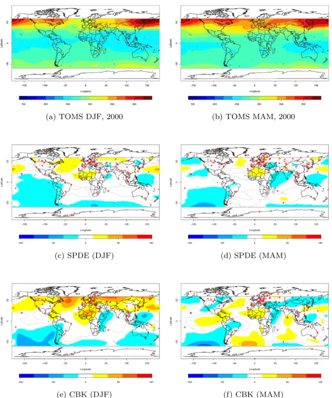
Figure 6.Ozone mapping from TOMS data in(a)DJF and(b)MAM; global difference mapping of SPDE and covariance-based kriging (CBK) predicted mean with respect to TOMS data in DJF (cande) and MAM (dandf) 2000.
timation in particular. In those circumstances, the SPDE ap-proach shows robustness against observations loss. Figures 6 and 7 show TOMS maps of all seasons in 2000 in top panels and differences with predictions from SPDE and covariance-based kriging. Underestimation at the South Pacific are in accordance with expectations for both techniques, but
sur-face predictions by SPDE achieve a better fit than covariance-based kriging, especially in SON.
4 Impact on long-term changes
(a) TOMS JJA, 2000 (b) TOMS SON, 2000
(c) SPDE (JJA) (d) SPDE (SON)
(e) CBK (JJA) (f) CBK (SON)
Figure 7.Ozone mapping from TOMS data in(a)JJA and(b) SON; global difference mapping of SPDE and covariance-based kriging (CBK) predicted mean with respect to TOMS data in JJA (cande) and SON (dandf) 2000.
SPDE-based mapping technique instead of covariance-based kriging.
4.1 Zonal mean time series analysis
To see how the ozone zonal means change over time over the same stations with different algorithms, we choose the sta-tions which supplied data for at least 25 years between 1979
Table 4.Generalized cross-validation error (σGCV) and residual sum of square (RSS) for different strategies over 2000–2005. Monthly and seasonally results are averaged over each year, and annual results are directly estimated using annual means from each station.
Year 2000 2001 2002 2003 2004 2005
Monthly n 143.25 151.58 147.50 136.17 135.25 138.42 A neff 34.42 19.20 35.73 31.49 20.76 27.65
σGCV 12.95 15.39 12.12 12.71 14.52 14.13 RSS 20 681 33 662 17 304 17 215 25 838 23 994
B neff 30.95 17.88 30.82 24.52 20.51 25.81 σGCV 10.85 12.60 10.34 10.98 12.75 11.72 RSS 14 473 23 946 12 693 13 930 20 112 15 998
C neff 75.34 51.17 76.18 76.03 52.61 58.57 σGCV 7.21 10.29 7.05 7.10 9.77 8.22 RSS 4157 12 734 3888 3019 9519 5906
D neff 81.27 47.06 80.41 78.16 55.88 70.26
σGCV 6.73 9.48 6.62 6.66 8.79 7.64
RSS 3306 10 890 3187 2692 6923 4574
Seasonally n 126.00 135.75 135.50 123.75 120.50 127.75 A neff 33.25 21.07 26.62 32.19 19.05 18.07 σGCV 10.44 11.67 9.17 9.23 9.99 12.18 RSS 9993 16 559 9306 7630 10 243 16 576
B neff 28.05 12.48 24.69 21.11 18.43 20.82 σGCV 8.18 10.38 7.71 8.37 8.63 9.63 RSS 6533 15 281 6552 7299 7781 9912
C neff 47.87 48.17 99.78 69.18 41.10 44.56
σGCV 5.23 8.51 5.58 5.31 6.78 7.39
RSS 2387 7546 1025 1567 4070 4695
D neff 63.11 55.65 84.82 68.48 51.23 55.28
σGCV 5.21 7.29 4.91 5.48 6.71 7.15
RSS 1888 5051 1372 1759 3507 3804
Annually n 83 97 101 90 87 97
A neff 27.90 15.96 9.94 10.43 6.02 3.00 σGCV 7.01 7.28 6.61 7.16 6.83 10.03
RSS 2704 4301 3982 4080 3782 9452
B neff 24.10 23.67 11.21 8.35 12.65 12.70
σGCV 5.05 5.34 6.29 7.23 5.95 8.67
RSS 1501 2094 3552 4271 2629 6342
C neff 47.32 40.50 48.22 57.58 25.63 28.00
σGCV 3.59 4.56 4.45 4.54 5.04 7.65
RSS 460 1172 1045 667 1556 4035
D neff 56.16 49.55 49.46 67.83 36.17 48.02
σGCV 3.12 4.08 4.56 4.93 5.03 7.11
RSS 261 790 1076 539 1469 3076
In order to overcome the underestimation over the South Pacific (see Fig. 4) and achieve a better estimation of long-term global zonal means, the monthly mean norms for each station were subtracted from observations over all the period. Then for each month, spatial interpolation through SPDE and covariance-based kriging were performed to the deviations.
The ozone norms were added back to these deviations in or-der to compare zonal means over the corresponding belts.
Table 6.Comparison with satellite data over all seasons and aver-aged over 2000–2005 RMSEs for covariance-based kriging (CBK) and SPDE predictions.
Season DJF MAM JJA SON Average
CBK 21.42 19.66 15.71 44.45 25.31
SPDE 18.45 13.54 8.49 9.20 12.42
Percentage of improvement 13.88 31.12 45.94 79.30 50.92
on ground-based data available from the WOUDC (Bo-jkov and Fioletov, 1995; Fioletov et al., 2002). The SBUV merged satellite data sets incorporated the measurements from eight backscatter ultraviolet instruments (BUV on Nim-bus 4, SBUV on NimNim-bus 7 and a series of SBUV/2 in-struments on NOAA satellites) processed with the v8.6 al-gorithm (Bhartia et al., 2013). The WOUDC ground-based zonal mean data set is based on the following technique. Firstly, monthly means for each point of the globe were es-timated from satellite TOMS data for 1978–1989. Then for each station and for each month the deviations from these means were calculated, and the belt’s value for a particular month was estimated as a mean of these deviations. The cal-culations were done for 5◦broad latitudinal belts. In order to take into account various densities of the network across regions, the deviations of the stations were first averaged over 5 by 30◦ cells, and then the belt mean was calculated by averaging these first set of averages over the belts. Un-til this point the data in the different 5◦belts were based on different stations (i.e., were considered independent). How-ever, the differences between nearby belts are small. Hence one can reduce the errors of the belt’s average estimations by using some smoothing or approximation. So the zonal means were then approximated by zonal spherical functions (Legendre polynomials cosine of the latitude) to smooth out spurious variations. This methodology (Bojkov and Fioletov, 1995) shares some ideas with SPDE in terms of taking advan-tage of spherical functions for spatial interpolation over the globe, but this methodology can only be conducted on zonal means calculation rather than global surface prediction. The merged satellite and the WOUDC data sets were compared again recently and demonstrated a good agreement (Chiou et al., 2014).
To investigate the pattern of zonal mean long-term changes in detail, Fig. 8 shows the monthly means from SBUV
Figure 8.Time series of zonal means by SBUV satellite data (black) WOUDC data set (green), covariance-based kriging (red) and SPDE (blue) from 1979 to 2010.
merged data (black), WOUDC data set (green), SPDE (blue) and based kriging (red). SPDE and covariance-based kriging estimated means both match well satellite data and the WOUDC data set in the Northern Hemi-sphere. Covariance-based kriging means in the tropics fluctu-ate heavily and are unrealistic in some years, which indicfluctu-ates that covariance-based kriging may perform well at some lo-cations but can provide distorted results at other lolo-cations; moreover the large kriging-based fluctuations in the begin-ning of the period may be due to a lack of stations in the early years of 1979–2010. SPDE estimated means are more robust under this circumstance. Limited stations in the South Hemi-sphere may trigger underestimation and deflation of the es-timated annual cycle in SPDE and covariance-based kriging. Therefore we carry out a seasonal smoothing by averaging September to November to estimate better the annual peak over the Southern Hemisphere (i.e., October). This smooth-ing algorithm improves the match with SBUV data.
4.2 Sensitivity analysis
(a) CBK zonal means (DU)
(b) SPDE zonal means (DU)
Figure 9.Time series of 30–60◦N zonal means by(a) covariance-based kriging (CBK) and (b) SPDE from 1990 to 2010 for four scenarios with 5, 10, 20 and 30 stations removed globally including 3, 6, 12 and 18 stations removed in the NH.
long-term ozone zonal mean change, we choose 57 stations (39 stations in the Northern Hemisphere, 10 stations in the tropics and 8 stations in the Southern Hemisphere) which provided data over the entire period from 1990 to 2010. We randomly remove 5, 10, 20 and 30 stations out of these set of stations by taking into account the relative weights of the respective regions and estimate the zonal mean trends in each case. The stations removed are randomly chosen by the de-sign in Table 7.
Furthermore, to illustrate possible variations in the sensi-tivity analysis, we randomly draw 5 sets of stations which need to be removed, labeled cases 1–5. The time series for different zonal mean trends over the latitude band 30–60◦N and 30–60◦S are displayed in Figs. 9 and 10, respectively.
(a) CBK zonal means (DU)
(b) SPDE zonal means (DU)
Figure 10.Time series of 30–60◦S zonal means by(a) covariance-based kriging (CBK) and(b) SPDE from 1990 to 2010 for four scenarios with 5, 10, 20 and 30 stations removed globally including 1, 2, 4 and 6 stations removed in the SH.
(a) SPDE annual zonal mean (b) CBK annual zonal mean
Figure 11.Annual zonal mean deviances from SBUV data (black), WOUDC data set (green), using all 57 available ground-based data (blue), random removed 5 (red), 10 (yellow), 20 (brown) and 30 (grey) stations in SPDE and covariance-based kriging (CBK) esti-mation over the (1) global (60◦N–60◦S), (2) NH (30–60◦N), (3) tropics (30◦N–30◦S) and (4) SH (30–60◦S) from 1990 to 2010.
Table 7.Design of the sensitivity analysis: stations to be removed are randomly selected within each region.
Number of removed 5 10 20 30 Total
NH (90–30◦N) 3 6 12 18 39 Tropics (30◦S–30◦N) 1 2 4 6 10
SH (30–90◦S) 1 2 4 6 8
We use case 1 for further illustration, where both SPDE and covariance-based approaches estimated well with respect to other cases. Figure 11 shows deviations in time series in the annual mean total ozone estimated by SBUV data, WOUDC data set, SPDE and covariance-based kriging. We can see that both SPDE and covariance-based kriging es-timate well in the Northern Hemisphere. Covariance-based kriging underestimates means significantly over the tropics and the Southern Hemisphere, while SPDE estimated means are close to SBUV trends. Note that SPDE estimated trends using all stations are closer to SBUV observations than the WOUDC data set at the tropics and Southern Hemisphere overall.
For the second part of sensitivity analysis, we add random long-term drifts into observations due to instrument-related problems. In reality, all observations from a ground-level sta-tion are often be biased by 5–10 DU (2–3 %) over a period of several years. For the setting of drifts, letyijbe the ozone
ob-(a) CBK zonal means (DU)
(b) SPDE zonal means (DU)
Figure 12.Time series of 30–60◦N zonal means by(a) covariance-based kriging (CBK) and(b) SPDE from 1990 to 2010 for four scenarios with 5, 10, 20 and 30 stations drifted globally.
servations at stationiand timej. We randomly select some stationsiand set
yij∗ =aiyij,
whereai∼N (1,0.032) is the slope over every 5-year
pe-riods, i.e., one slope factor for 1990–1994, then different drifts for 1995–1999, 2000–2004 and 2005–2010. This set-ting means that stations were randomly selected and drift val-ues were then randomly generated, but the drifts are fixed for each particular station over every 5 or 6 years.
vari-(a) CBK zonal means (DU)
(b) SPDE zonal means (DU)
Figure 13.Time series of 30–60◦S zonal means by(a) covariance-based kriging (CBK) and (b) SPDE from 1990 to 2010 for four scenarios with 5, 10, 20 and 30 stations drifted globally.
ations in the selection process. The time series in each case are shown in Figs. 12 and 13 for the Northern and South-ern Hemisphere. Covariance-based kriging estimations hold in the case of over half of stations are drifted, SPDE also displays robustness to drift. We use case 1 as further illus-tration. Figure 14 shows the annual mean total ozone de-viations in time series for SBUV, WOUDC data set, SPDE and covariance-based kriging estimated means when drifts are present. SPDE estimated trends turn out to be superior to covariance-based kriging over the tropics and Southern Hemisphere overall.
Table 8 reports monthly, seasonal and annual average RMSEs obtained by comparing the WOUDC, SPDE and covariance-based kriging estimated zonal means to the SBUV zonal means over 1990–2010. We can see that SPDE
(a) SPDE annual zonal means (b) CBK annual zonal means
Figure 14.Annual zonal mean deviances from SBUV data (black), WOUDC data set (green), using all 57 available ground-based data (blue), adding drift to 5 (red), 10 (yellow), 20 (brown) and 30 (grey) stations in SPDE and covariance-based kriging (CBK) estimation over the (1) global (60◦N–60◦S), (2) NH (30–60◦N), (3) tropics (30◦N–30◦S) and (4) SH (30–60◦S) from 1990 to 2010.
5 Conclusions
Appendix A: Computational details of SPDE and covariance-based approaches
A1 SPDE approach
The algorithm of estimation of parameters in SPDE works as follows. LetY (s)be an observation of the latent fieldP (s)+ X(s), the model is given by
Y (s)=P (s)+X(s)+ǫ(s),
whereP is a polynomial which is the fixed part of the model,
X(s)is the solution of the SPDE (Eq. 3) and observation er-rorǫ(s)is zero mean Gaussian noise with varianceσ2. This fieldX(s)can be built on a basis representation
x(s)=
n
X
k=1
ψk(s)wk,
where wk is the stochastic weight chosen so that the x(s)
approximates the distribution of solutions to the SPDE on the sphere. The basis functions ψk(s) are chosen by a
fi-nite element method in order to obtain a Markov structure and to preserve it when conditioning on local observations. To allow an explicit expression of the precision matrix for the stochastic weights, we use a piecewise linear basis func-tions for the location of the observafunc-tions. The overall ef-fect of the mesh construction is that smaller triangles indi-cate higher accuracy of the field representation, where the observations are more dense, such as the network at the Northern Hemisphere. Larger triangles are constructed in the Southern Hemisphere as observations are more sparse, thus we can preserve computational resources. In order to bal-ance the local accuracy and computational tractability, we add some triangles with the following restrictions. The mini-mum allowed distance between points is 10/rkm (r=6371 is the Earth radius) and the maximum allowed edge length in any triangle is 500/rkm, with the aim to refine the trian-gulation into an embedded spherical mesh. LetC= hψi, ψji
andG= h∇ψi,∇ψjibe matrices used in the construction of
the finite element solutions of the SPDE approach. Then for
α=2, the precision matrix for the weights{wi}is given by
Q=τ2(κ4C+2κ2G+GC−1G),
where the elements ofQhave explicit expressions as func-tions ofκ2andτ (Lindgren et al., 2011).
As pointed out in Jun and Stein (2008), the spatial mean structure on a sphere can be modeled using a regression ba-sis of spherical harmonics; however, since the data set only contains measurements from one specific event, it is not pos-sible to identify which part of the variation in the data come from a varying mean and which part can be explained by the variance–covariance structure of the latent field. To obtain basic identifiability, the parameters κ(s)andτ (s)are taken
to be positives, and their logarithm can be decomposed as logκ(s)=X
k, m
κk, mSk, m(s),
logτ (s)=X
k, m
τk, mSk, m(s),
whereSk, m is the spherical harmonic of orderkand mode
m. The real spherical harmonicSk, m(s)of orderk∈N0and
modem= −k, . . ., kis defined as
Sk, m(s)=
s 2k+1
4π
(k− |m|)! (k+ |m|)!
√
2 sin(ml)Pk,|m|(sinL) if −k≤m<0,
Pk,0(sinL) ifm=0,
√
2 cos(ml)Pk, m(sinL) if 0<m≤k,
wherePk, mare associated Legendre polynomials:
Pk, m(x)=(−1)m(1−x2)m/2
dm
dxmPk(x),
wherePk are Legendre polynomials,
Pk(x)=
1 2kk!
dk
dxk(x 2
−1)k.
Regarding the computational implementation of the SPDE approach, one common choice would be to use a Metropolis– Hastings algorithm, which is easy to implement but computa-tionally inefficient (Bolin and Lindgren, 2011). A better way is to use direct numerical optimization to estimate the pa-rameters by employing the INLA framework, available as an R package (http://www.r-inla.org/). The default value in R-INLA isα=2, but 0≤α<2 are also available, though yet to be completely tested (Lindgren and Rue , 2015). So with
α=2 and a spherical two-manifold, the smoothness param-eterνmust be fixed at 1 due to the relationshipα=ν+d/2. A2 Covariance-based approach
i=1
Furthermore, to choose the number of basis functions for
κ(s) andτ (s)in an SPDE and to compare the performance of SPDE and covariance-based approaches, we also used the GCV criterion (Wahba, 1985). Let yˆ be the predictor vector for the observed y withyˆ=A(λ)y, where Ais the
n×n smoothing matrix, and let the neff=trA(λ) measure
the effective number of degrees of freedom attributed to the smooth surface, which is also called the effective number of parameters. The GCV criterion selectsλas the minimizer of the GCV function:
V (λ)= n
−1k(I−A(λ)y)k [n−1tr(I−A(λ))]2 =
1
n
n
X
i=1
y
i− ˆyi
1−tr(A(λ))/n
2
.
In practice, the GCV function computes the weighted residual sum of squares when each data point (i.e., station) is omitted and predicted from the remaining points. The value ofλis linked to SPDE and covariance-based kriging by min-imizing the GCV function. This allows the selection of the best λ according to fit of predictions while accounting for possible overfitting due to a large number of parameters used. After the optimalλis selected, the weighted residual vari-anceσGCV2 is defined as
σGCV2 =
Pn
i=i(yi− ˆyi)2
n−tr(A(λ)) . (B2)
Acknowledgements. Kai-Lan Chang was supported by the Tai-wanese government sponsorship for PhD overseas study. S. Guillas was partially supported by a Leverhulme Trust research fellowship on stratospheric ozone and climate change (RF/9/RFG/2010/0427).
Edited by: L. Bianco
References
Bhartia, P. K., McPeters, R. D., Flynn, L. E., Taylor, S., Kramarova, N. A., Frith, S., Fisher, B., and DeLand, M.: Solar Backscatter UV (SBUV) total ozone and profile algorithm, Atmos. Meas. Tech., 6, 2533–2548, doi:10.5194/amt-6-2533-2013, 2013. Bojkov, R. D. and Fioletov, V. E.: Estimating the global ozone
char-acteristics during the last 30 years, J. Geophys. Res.-Atmos., 100, 16537–16551, doi:10.1029/95JD00692, 1995.
Bolin, D. and Lindgren, F.: Spatial models generated by nested stochastic partial differential equations, with an application to global ozone mapping, Ann. Appl. Stat., 5, 523–550, doi:10.1214/10-AOAS383, 2011.
Chiou, E. W., Bhartia, P. K., McPeters, R. D., Loyola, D. G., Coldewey-Egbers, M., Fioletov, V. E., Van Roozendael, M., Spurr, R., Lerot, C., and Frith, S. M.: Comparison of profile total ozone from SBUV (v8.6) with GOME-type and ground-based total ozone for a 16-year period (1996 to 2011), Atmos. Meas. Tech., 7, 1681–1692, doi:10.5194/amt-7-1681-2014, 2014. Fioletov, V. E., Labow, G., Evans, R., Hare, E., Köhler, U.,
McEl-roy, C., Miyagawa, K., Redondas, A., Savastiouk, V., Shala-myansky, A., Staehelin, J., Vanicek, K., Weber, M.: Per-formance of the ground-based total ozone network assessed using satellite data, J. Geophys. Res.-Atmos., 113, D14313, doi:10.1029/2008JD009809, 2008.
Fioletov, V. E., Bodeker, G. E., Miller, A. J., McPeters, R. D., and Stolarski, R.: Global and zonal total ozone variations estimated from ground-based and satellite measurements: 1964–2000, J. Geophys. Res., 107, ACH 21-1–ACH 21-14 doi:10.1029/2001JD001350, 2002.
Frith, S. M., Kramarova, N. A., Stolarski, R. S., McPeters, R. D., Bhartia, P. K., and Labow, G. J.: Recent changes in column ozone based on the SBUV version 8.6 merged ozone dataset, J. Geo-phys. Res., 119, 9735–9751, doi:10.1002/2014JD021889, 2014. Gneiting, T.: Strictly and non-strictly positive definite functions on spheres, Bernoulli, 19, 1327–1349, doi:10.3150/12-BEJSP06, 2013.
Guinness, J. and Fuentes, M.: Covariance functions for mean square differentiable processes on spheres, submitted, 2013.
Jun, M. and Stein, M. L.: An approach to producing space-time covariance functions on spheres, Technometrics, 49, 468–479, doi:10.1198/004017007000000155, 2007.
Jun, M. and Stein, M. L.: Nonstationary covariance models for global data, Ann. Appl. Stat., 2, 1271–1289, doi:10.1214/08-AOAS183, 2008.
Lindgren, F., Rue, H., and Lindström, J.: An explicit link between Gaussian fields and Gaussian Markov random fields: the stochas-tic partial differential equation approach, J. Roy. Stat. Soc. B, 73, 423–498, doi:10.1111/j.1467-9868.2011.00777.x, 2011. Lindgren, F. and Rue, H.: Bayesian spatial and spatiotemporal
modelling with R-INLA, J. Stat. Softw., 63, 19, 2015.
Stein, M. L.: Space-time covariance functions, J. Am. Stat. Assoc., 100, 310–321, doi:10.1198/016214504000000854, 2005. Stein, M. L.: Spatial variation of total column ozone on a global
scale, Ann. Appl. Stat., 191–210, doi:10.1214/07-AOAS106, 2007.