Vol. 3, No. 1, June 2006, 63 - 76
Dynamic Performances of Self-Excited Induction
Generator Feeding Different Static Loads
Ali Nesba1, Rachid Ibtiouen2, Omar Touhami3
Abstract: The paper examines the dynamic performances of a three-phase self-excited induction generator (SEIG) during sudden connection of static loads. A dynamic flux model of the SEIG in the ˺-˻ axis stationary reference frame is presented. The main flux saturation effect in the SEIG is accounted for by using an accurate technique. The cases of purely resistive, inductive and capacitive load are amply discussed. Models for all of these three-phase load in the ˺-˻ axis stationary reference frame are also given. The analysis presented is validated experimentally.
Keywords: Induction generator, Self-excitation, Dynamic performances, Loading conditions.
1
Introduction
The induction generator self-excitation phenomenon has been well known since the beginning of the last century. Bassett and Potter [1] published their work on this subject and explained the self-excitation process. They demonstra-ted that an externally driven induction machine can operate as a generator if a reactive power source is available to provide the machine's excitation. The self-excitation can be achieved when a capacitor bank with an appropriate value is properly connected across the machine terminals.
In recent years, self-excited induction generator has been widely used as suitable power source, particularly in renewable power generating systems, such as in hydroelectric and wind energy applications [2-8].
Robust and brushless construction (squirrel cage rotor), low maintenance requirements, absence of DC power supply for field excitation, small seize, re-duced cost, better transient performance, self-protection against short-circuits and large over loads, are some of the advantages of the induction generator over the synchronous and DC generators. The disadvantages of this type of generator are its relatively poor voltage and frequency regulation, and low power factor.
1Laboratory of Electrical Engineering, Ecole Nationale Polytechnique, ENP, BP 182 El-Harrach 16200 Algiers, Algeria; E-mail: [email protected]
The frequency and magnitude of voltage generated by the SEIG is highly influenced by the rotor speed, the excitation and the load [7,8].
The steady state analysis of the isolated SEIG has been extensively dealt with over the last decades. However, the literature on the analysis of the dynamic performance of the isolated SEIG, particularly under different loading conditions, appears to be somewhat sparse.
The aim of this paper is to present an analysis of the dynamic performance of an isolated three-phase SEIG feeding four types of three-phase static loads; resistive (R), resistive-inductive (RL), resistive-capacitive (RC) and resistive-inductive-capacitive loads (RLC).
The dynamic flux models of the SEIG as well as the models of R, RL, RC
and RLC loads are given. The analysis presented is validated by experimental results.
2
Induction Generator Model
The induction machine voltage equations in the ˺ − ˻ axis stationary reference frame may be expressed [9]:
s s s s
d = r +
v i
dt ˺
˺ ˺
̞
(1)
s s s s
d = r +
v i
dt ˻
˻ ˻
̞
(2)
r r r r r r
d
= r i +
v
dt ˺
˺ ˺ ˻
′ ̞
′ ′ − ̒ ̞′ (3)
r r r r r r
d
= r i +
v
dt ˻
˻ ˻ ˺
′ ̞
′ ′ + ̒ ̞′ (4)
All rotor quantities and parameters are referred to the stator: – ̒ris the angular speed of the rotor.
– v˺s, v˻s, v˺′r and v˻′r denote the ˺ − ˻ axis components of the stator, and rotor voltages referred to the stator respectively;
– i˺s, i˻s, i˺′r and i˻′r represent the ˺ − ˻ axis components of the stator, and rotor currents referred to the stator respectively;
– ̞˺s, ̞˻s, ̞˺′r and ̞˻′r represent the ˺ − ˻ axis components of the stator, and rotor fluxes referred to the stator respectively; and
s m s s - = i l ˺ ˺ ˺ ̞ ̞
, (5)
˻s m˻ ˻s s - = i l ̞ ̞
, (6)
r m r
r
- i =
l ˺ ˺ ˺ ′ ̞ ̞ ′
′ , (7)
r m˻ r
r
- i =
l ˻ ˻ ′ ̞ ̞ ′
′ , (8)
where:
− ls and l′r denote stator and rotor leakage inductances referred to the stator;
− ̞m˺ and ̞m˻ which are useful quantities when representing saturation, denote the ˺ and ˻-axis components of the magnetizing flux:
( s r)
m˺ = M i˺ + i˺′
̞ , (9)
( s r)
m˻ = M i˻ + i˻′
̞ , (10)
3 2 ms
M = L , (11)
−and Lms represents the stator magnetizing inductance.
The use of (5)-(8) helps to eliminate the currents in (9) and (10) as well as in the voltage equations given by (1)-(4), and if the resulting voltage equations are solved for the ˺ − ˻ axis fluxes, the following state equations can be obtained:
(
)
s s
s m s
s d r v dt l ˺ ˺ ˺ ˺ ̞
= + ̞ − ̞ (12)
(
)
s s
s m s
s d r v dt l ˻ ˻ ˻ ˻ ̞
= + ̞ − ̞ (13)
(
)
r r
r r r m r
r d r v dt l ˺ ˺ ˻ ˺ ˺ ′ ′ ̞ ′ ′ ′ = + ̒ ̞ + ̞ − ̞ ′ (14)
(
)
r rr r r m r
r d r v dt l ˻ ˻ ˺ ˻ ˻ ′ ̞ ′ ′ ′ ′ = + ̒ ̞ + ̞ − ̞
′ . (15)
1
s
s e
dv
= i
dt C
˺
˺ , (16)
1
s
s e
dv
= i
dt C
˻
˻ , (17)
where Ce denotes excitation capacitor.
If the studied induction generator is assumed to be magnetically linear, the SEIG flux model, in the stationary reference frame, may be obtained by the use of the magnetizing flux expressions (9), (10), the set of conventional state equations (12)-(15) and the self-excitation equations (16), (17).
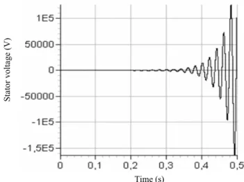
However, the modeling of the SEIG under the assumption of magnetic linearity leads to unrealistic results. Fig. 1 shows the influence of neglecting the saturation effect in the simulation and particularly the computed stator voltage during the self-excitation process. It can be seen that the voltage reaches thousands of volts in less then half a second. This computed result cannot be obtained experimentally, because the SEIG output voltage is limited by the magnetic saturation phenomenon. The following section presents briefly the method used in this paper, to take into account the saturation effect.
Time (s)
S
ta
to
r
v
o
lt
ag
e
(V)
Fig. 1 – Computed stator voltage during the self-excitation process when the saturation effect is neglected.
3
Saturation Model
polynomial and arctangent functions were used in this model in order to obtain a maximum of accuracy. An optimization least-square method was applied for the determination of the model coefficients. This model is expressed as follow
0
0
if
if
l m s m
M I I
M
M I I
≤ =
> (18)
where:
− Ml is the value of the magnetizing inductance of the machine in the linear region;
− Ms is the expression of the magnetizing inductance in the saturated region, and is given by
3
2 0 0 4 0 5
arctan( ( )) ( exp( ( ))) ( )
s 1 m m m
M C= C I −I C 1+ − − I −I C I+ −I +C ;
(19)
− Im denotes the rms magnetizing current; I0 is the value of Im at the upper limit of the linear region.
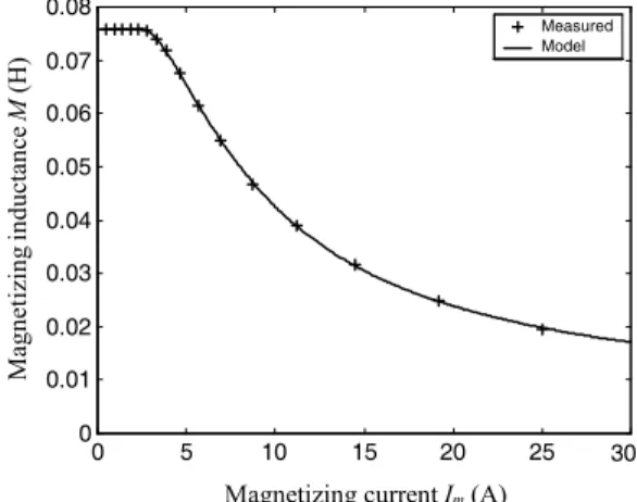
The coefficients Ci (i=1,…,5),
0
I and Ml are identified by using a least-square optimization method. Relative difference between tests data and the model of M is within exp(-6). Model-based computed values and measured values of the magnetizing inductance as a function of the magnetizing current are shown in the Fig. 2.
0 5 10 15 20 25 30
0 0.01 0.02 0.03 0.04 0.05 0.06 0.07 0.08
Measured Model
Magnetizing currentIm (A)
M
ag
n
et
iz
in
g
in
d
u
ct
an
ce
M
(
H
)
Fig. 2 – Variation of the saturated magnetization inductance of the studied machine versus the magnetizing current.
and ˻-magnetizing flux components ̞m˺and ̞m˻. These components may be expressed by
s r m
s r
= L +
l l
˺ ˺
˺ ˺
′ ̞ ̞ ̞
′ , (20)
s r m
s r
= L +
l l
˻ ˻
˻ ˻
′
̞ ̞
̞
′ , (21)
-1
s r
1 1 1
L = L + +
M l l
˺ ˻ = ′ . (22)
Obviously,L˺, L˻ and consequently ̞m˺ and ̞m˻ are related to the
magne-tizing inductance M which is a function of the rms magnetizing current (18), (19).
This current is given by
( 2 2 ) / 2
m m m
I = i i˺ + ˻ , (23)
where
m s r
i ˺ =i˺ +i˺′ (24)
and
m s r
i i i˻= ˻ + ˻′ (25)
Finally, the saturated flux model of SEIG, in the stationary reference frame, is obtained by adding the expressions of the magnetizing inductance, fluxes and currents (18)-(25), to the equations of the linear model presented in the previous section.
4
Experimental Verification
In this section, experimental and computed results are presented. These results (Figs. 3-13) describe the dynamic responses of the studied induction generator during sudden connection of three-phase static loads onto the machine terminals. The machine used for the tests is a wound-rotor induction machine rated: 3.5kW, 220/380V, 14/8A, 50Hz, 4 poles.
4.1 Resistive load
The model of a three-phase balanced resistive load in the ˺-˻ axis stationary reference frame is given by:
L
v˺ =Ri ˺, (26)
and
L
v˻ =Ri ˻, (27)
where:
− R is the load resistance (per phase);and
−iL˺ and iL˻ are respectively the ˺and ˻-axis components of the load current.
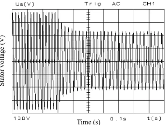
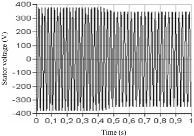
Figs. 3 and 5 show the measured stator voltage and stator current following a sudden connection of the load (R=15˲). The computed results are given in Figs. 4 and 6. Both computed and measured results show that a large voltage drop occurs when the load is connected onto the SEIG terminals.
Time (s)
S
ta
to
r
v
o
lt
ag
e
(
V
)
Fig. 3 – Measured stator voltage during the connection of load.
S
ta
to
r
v
o
lt
a
g
e
(
V
)
Time (s)
S
ta
to
r
cu
rr
en
t
(A
)
Time (s)
Fig. 5 – Measured stator current during the connection of load.
Time (s)
S
ta
to
r
cu
rr
en
t
(A
)
Fig. 6 – Computed stator current during the connection of load.
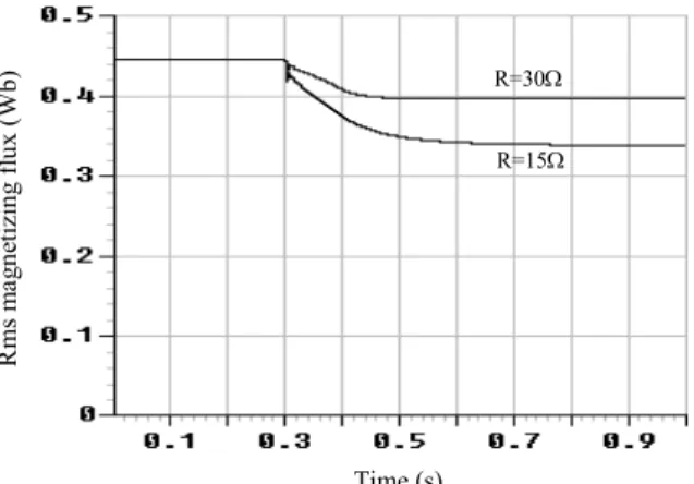
The Fig. 7 shows the effect of the load resistance (impedance) on the rms
magnetizing flux. It describes the rms magnetizing flux during the self-excitation process and the perturbation provoked by the load (at 0.3s). Cases of 15˲ and
30˲ resistive loads are examined.
4.2 Inductive load
The dynamic model of a three-phase balanced series RL (resistive-induc-tive) load in the ˺-˻ axis stationary reference frame is expressed by
( ) /
L
L
di
= v - Ri L
dt ˺
˺ ˺ (28)
and
( ) /
L
L
di
= v - Ri L
dt ˻
R and L are the load resistance and inductance (per phase) respectively. The inductive loads used in this paper (in RL and RLC loads) are magnetically linear, and present no magnetic coupling between phases.
Time (s)
R
m
s
m
a
g
n
et
iz
in
g
f
lu
x
(
W
b
) R=30˲
R=15˲
Fig. 7 – Computed rms magnetizing flux during the connection of load.
S
ta
to
r
v
o
lt
ag
e
(V
)
Time (s)
Fig. 8 – Measured stator voltage during the connection of load.
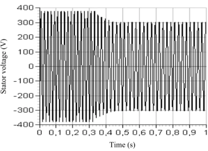
The Fig. 8 shows the measured stator voltage following a sudden connection of the inductive load (R = 47.5˲, L = 0.12H). The computed result is given in Fig. 9. Although the resistive part of this load (47.5˲) is over than three times greater than the resistance in the case of resistive load (15˲), computed and measured results still showing a large voltage drop after the connection of the load.
reactance of the generator to increase. On the other hand, it engenders some voltage drop in the stator windings, which consequently causes the voltage across the excitation capacitors to decrease, and, as a result, the reactive power produced by these capacitors also decrease. This diminution in the reactive power produced by the SEIG (capacitors), in addition to the increase of the demand of reactive power, constrain the SEIG to operate with weak excitation and thus, with lower output voltage
Time (s)
S
ta
to
r
v
o
lt
ag
e
(V
)
Fig. 9 – Computed stator voltage during the connection of load.
4.3 Capacitive load
One improvement of the SEIG output voltage characteristic is based on using capacitors in series and/or in parallel with the load. In this paper, only series connection is considered. The dynamic performance of the SEIG, feeding series connected RC and RLC loads, is examined.
The dynamic model of a three-phase balanced series RC (resistive-capa-citive) load in the ˺-˻ axis stationary reference frame can be written:
1
( )
C
C
dv
v v
dt RC
˺
˺ ˺
= − , (30)
and
1
( )
C
C
dv
v v
dt RC
˻
˻ ˻
= − , (31)
where:
− R and C are the load resistance and capacitance (per phase), respectively;
− vC˺and vC˻ are respectively, the ˺- and ˻-axis components of the voltage
The measured and computed results in Figs. 10 and 11 show the output voltage during the connection of RC load onto the SEIG terminals. Although the impedance of the test RC load (15 ˲, 135 HF) is less than a half of the RL load impedance (47.5 ˲, 0.12 H), it can be clearly seen that the connection of this RC
load has no significant effect on the generator output voltage. In fact, the deficit in the SEIG reactive power, caused by the connection of the load, and which is directly related to the load power factor and impedance may be compensated by the use of series capacitors with the load.
S
ta
to
r
v
o
lt
ag
e
(V
)
Time (s)
Fig. 10 – Measured stator voltage during the connection of load.
Time (s)
S
ta
to
r
v
o
lt
ag
e
(V
)
Fig. 11 – Computed stator voltage during the connection of load.
4.4
RLC
load
2
2 0
C C
C
d v dv
LC RC v v
dt dt
˺ ˺
˺ ˺
+ + − = , (32)
2
2 0
C C
C
d v dv
LC RC v v
dt dt
˻ ˻
˻ ˻
+ + − = , (33)
where R, L and C are the load resistance, inductance and capacitance (per phase), respectively.
S
ta
to
r
v
o
lt
ag
e
(V
)
Time (s)
Fig. 12 – Measured stator voltage during the connection of load.
Time (s)
S
ta
to
r
v
o
lt
ag
e
(V
)
Fig. 13 – Computed stator voltage during the connection of load.
This can be referred to the low value of the series capacitor relatively to the load impedance and power factor. In fact, the series capacitor used with the load, must have an appropriate capacitance value, so that it can maintain sufficient excitation for the SEIG when the load is connected. On the other hand, a higher value capacitor will overexcite the SEIG, and the output voltage can reach dangerous values.
5
Conclusion
An analysis on the dynamic performance of an isolated three-phase SEIG feeding four kinds of three-phase static loads is presented. The cases of R, RL,
RC and RLC loads are considered.
The dynamic flux models of the SEIG as well as the models of R, RL, RC
and RLC loads in the ˺ − ˻ axis stationary reference frame are given. The main flux saturation effect in the SEIG is accounted for by using accurate technique. The analysis presented is validated by experimental results.
The connection of a load onto the SEIG terminals causes its excitation to decrease and thus, the SEIG to operate at lower magnetizing flux. The SEIG output voltage is highly influenced by the impedance and the power factor of the load.
The use of series capacitor with the load, improves considerably the output voltage characteristic of the SEIG. This series capacitor must have an adequate capacitance value.
The amplitudes of the signals, their shapes as their duration present practically the same values for both simulation and experimentation.
The coherence between computed and measured results is very good as well for dynamic conditions as for steady state. This concordance between the experimentation and simulation confirms the validity of the developed models.
6
References
[1] E. D. Basset, F.M. Potter: Capacitive Excitation of Induction Generators: Trans. Amer. Inst. Electr. Eng., 54, 1935, pp. 540–545.
[2] T. Ahmed, O. Noro, E. Hiraki, M. Nakaoka: Terminal Voltage Regulation Characteristics by Static Var Compensator for a Three-Phase Self-Excited Induction Generator: IEEE Trans. on Industry Applications, Vol. 40, No. 4, 2004, pp. 978–988.
[3] S.A. Daniel, N. A.Gounden: A novel hybrid isolated generating system based on pv fed inverter-assisted wind-driven induction Generators, Trans. on Energy Conversion, Vol. 19, No. 2, 2004, pp. 416–422.
[5] B. Palle, M.G. Simoes, F.A. Farret: Dynamic Simulation and Analysis of Parallel Self-Excited Induction Generators for Islanded Wind Farm Systems, IEEE Trans. on Industry Applications, Vol. 41, No. 4, 2005, pp. 1099–1106.
[6] R. Ibtiouen, A. Nesba, S. Mekhtoub, O. Touhami: An approach for the modeling of saturated induction machine, Proc. International AEGAN Conference on Electrical Machines and Power Electronics, ACEMP'01, Kasudasi-Turkey, 27-29 June, 2001, pp. 269–274.
[7] G.K. Singh: Self-excited induction generator research-a survey, Electric Power Systems Research, 69, 2004, pp. 107–114.