Abs tract
In this paper, the effect of the temperature change on the vibra-tion frequency of mono-layer graphene sheet embedded in an elas-tic medium are studied. Using the nonlocal elaselas-ticity theory, the governing equations are derived for single-layered graphene sheets. Using Levy and Navier solutions, analytical frequency equations for single-layered graphene sheets are obtained. Using Levy solu-tion, the frequency equation and mode shapes of orthotropic rec-tangular nanoplate are considered for three cases of boundary conditions. The obtained results are subsequently compared with valid result reported in the literature. The effects of the small scale, temperature change, different boundary conditions, Winkler and Pasternak foundations, material properties and aspect ratios on natural frequencies are investigated. It has been shown that the non-dimensional frequency decreases with increasing temperature change. The present analysis results can be used for the design of the next generation of nanodevices that make use of the thermal vibration properties of the nanoplates.
Key words
Thermo-mechanical vibration; Orthotropic single-layered graphene sheets; Elastic medium; Analytical modeling.
Exact solution for thermo-mechanical vibration of
or-thotropic mono-layer graphene sheet embedded in an
elastic medium
1 INTRODUCTION
Nano-materials have attracted attention of many researchers in this field due to their novel prop-erties. Many scientific communities study the characteristics of nanomaterials such as carbon nanotubes (CNTs), nanoplates, nanorods and nanorings. To design plate efficiently, we need to understand their vibration behavior. Vibration of ‘scale-free’ plates has been studied widely in the literatures which this theory cannot predict the size effects. Thus, in with small size, long-range inter-atomic and inter-molecular, cohesive forces cannot be ignored because they strongly affect
M. Mo ham m adi a , b * A . Mo ra di a
M. G h ayo ur b A . Faraj p our b
a Department of engineering, Ahvaz branch,
Islamic Azad University, Ahvaz, Iran.
b
Department of mechanical engineering, Isfa-han University of Technology, IsfaIsfa-han 84156-83111, Iran.
Received in 24 Mar 2013 In revised form 12 Jun 2013
Latin American Journal of Solids and Structures 11 (2014) 437 - 458
the static and dynamic properties (Wong et al 1997; Sorop and Jongh 2007). To use graphene sheets properly as design nano electro-mechanical system and micro electro-mechanical systems (NEMS and MEMS) component, their frequency response with small-scale effects should be inves-tigated.
Graphene is a truly two-dimensional atomic crystal with exceptional electronic and mechanical properties. Many nanostructures based on the carbon such as carbon nanotube (Iijima 1991), nanorings (Kong et al 2004), etc. are considered as deformed graphene sheet so analysis of gra-phene sheets is a basic matter in the study of the nanomaterials.
Latin American Journal of Solids and Structures 11 (2014) 437 - 458 have been reported on the mechanical properties. However, compared to the nanotubes, studies for the nanoplates are very limited, particularly for the mechanical properties with thermal ef-fects.
In the present study, the effect of the temperature change on the vibration frequency of ortho-tropic monolayer graphene sheets embedded in an elastic medium is investigated. The governing equations of motion are derived using the nonlocal elasticity theory. Levy type solution for the vibration of orthotropic rectangular nanoplate under thermal effect and elastic medium is ob-tained. Unlike the case of an isotropic plate that the roots are easily seen repeated roots but for this case there are four sets because the roots depend on the relative stiffness of the nanoplate in various directions, effect of elastic medium and temperature change. Hence, in this study for the thermal vibration of orthotropic rectangular nanoplate in an elastic medium using the Levy-type solution requires four different forms for the homogeneous solution. The small scale effects and thermal effect on the vibrations frequency of graphene sheets with three set boundary conditions are investigated. The thermal effects, effect of boundary condition and some other impressions on the vibration properties are investigated. From the results, some new and absorbing phenomena can be observed. To suitably design nano electro-mechanical system and micro electro-mechanical systems (NEMS/MEMS) devices using graphene sheets, the present results would be useful. 2 N O N LO C A L P LA T E M O D E L
The nonlocal elasticity theory was introduced by Eringen (1983). In this theory, the stress state at a given point depends on the strain states at all points, while in the local theory, the stress state at any given point depends only on the strain state at that point. Stress components for a linear homogenous nonlocal elastic body without the body forces using nonlocal elasticity theory, we have (Eringen 1983):
(
)
( )
,
(
)
(
),
ij
x
x x
C
ijkl klx dV x
σ
=
∫
λ
−
′
γ
ε
′
′
∀ ∈
x
V
,
(1)where
σ
ij,
ij
ε
andijkl
C
are the stress, strain and fourth order elasticity tensors, respectively. The termλ
(
x
−
x
′
,
γ
)
is the nonlocal modulus (attenuation function) incorporating into constitutive equations the nonlocal effects.γ
(�=�!�! �) is a material constant that depends on the internal
a
(lattice parameter, granular size, distance betweenC
−
C
bonds), and external characteristics lengthsl
(crack length, wave length),l
. Choice of the value of parametere
0 is vital for theLatin American Journal of Solids and Structures 11 (2014) 437 - 458
(
)
(
2 2)
[ ]
{ } { }
0
1
nli
e l
σ
C
ε
λ
T
−
∇
=
⎡
⎣
−
Δ
⎤
⎦
(2)where nl
σ
,ε
, andλ
denote the nonlocal stress, strain, and stress–temperature coefficients vec-tors, respectively.Δ
T
is the temperature change, C denote the elastic stiffness tensor.∇
2 is the Laplacian operator that is defined by 2 2 2 2 2(
/
x
/
y
).
∇
=
∂
∂
+
∂
∂
The nonlocal constitutive equa-tion Eq. (2) has been lately employed for the study of micro- and nano-structural elements. We consider nano monolayer orthotropic graphene sheets in our present study. In two-dimensional forms Eq. (2) are written as (Malekzadeh et al 2011):1 12 21 12 2 12 21 2 2
0 12 2 12 21 2 12 21
12
/ ( 1
)
/ ( 1
)
0
(
)
/ ( 1
)
/ ( 1
)
0
0
0
2
nl nl
xx xx xx xx
nl nl
yy i yy yy yy
nl nl
xy
xy xy
E
E
T
e l
E
E
T
G
σ
σ
υ υ
υ
υ υ
ε
α
σ
σ
υ
υ υ
υ υ
ε
α
ε
σ
σ
⎧
⎫
⎧
⎫
⎡
−
−
⎤
⎧
−
Δ
⎫
⎪
⎪
−
∇
⎪
⎪
⎢
⎥
⎪
⎪
=
−
−
−
Δ
⎨
⎬
⎨
⎬
⎢
⎥
⎨
⎬
⎪
⎪
⎪
⎪
⎢
⎥
⎪
⎪
⎣
⎦ ⎩
⎭
⎩
⎭
⎩
⎭
(3)
where
E
1 andE
2 are the Young’s modulus, and12
G
is shear modulus, 12υ
and21
υ
indicate Poisson’s ratio , andα
xxand
α
yy are the coefficient of thermal expansion along the principlematerial directions
x
andy
, respectively. The strains in terms of displacement components inthe middle surface can be written as follows (Malekzadeh et al 2011):
2 2 2
0 0 0 0
2 2
1
,
,
2
2
xx yy xx
u
w
v
w
u
v
w
z
z
z
x
x
y
y
y
x
x y
ε
=
∂
−
∂
ε
=
∂
−
∂
ε
=
⎛
⎜
⎛
⎜
∂
+
∂
⎞
⎟
−
∂
⎞
⎟
∂
∂
∂
∂
⎝
⎝
∂
∂
⎠
∂ ∂
⎠
(4)In the foregoig, the first terms on the right-hand sides of the above equations represent the strain components in the middle surface due to its stretching, and terms with w represent the strain components due to bending. Stress resultants are defined as below for development of rec-tangular nanoplate (Pradhan and Phadikar 2009).
/ 2 / 2
,
h nl xx xx hN
σ
dz
−
=
∫
/ 2 / 2,
h nl yy yy hN
σ
dz
−
=
∫
/ 2 / 2,
h nl xy xy hN
σ
dz
−
=
∫
/ 2 / 2,
h nl xx xx hM
z
σ
dz
−
=
∫
/ 2 / 2,
h nl yy yy hM
z
σ
dz
−
=
∫
/ 2 / 2 h nl xy xy hM
z
σ
dz
−
=
∫
(5)
Latin American Journal of Solids and Structures 11 (2014) 437 - 458
2 2
2 2
0 11 2 12 2
(
)
,
xx i xx
w
w
M
e l
M
D
D
x
y
∂
∂
−
∇
=
−
−
∂
∂
2 2 2 20 12 2 22 2
(
)
yy i yy
w
w
M
e l
M
D
D
y
x
∂
∂
−
∇
=
−
−
∂
∂
2 2 2 0 66(
)
2
,
xy i xy
w
M
e l
M
D
x y
∂
−
∇
=
−
∂ ∂
(6)
where
D
ij indicate the different bending rigidity is defined as (Pradhan and Phadikar 2009):11 1 12 21
2
12 12 2 12 21 2
22 2 2 12 21
66 12
/ ( 1
)
/ ( 1
)
/ ( 1
)
h h
D
E
D
E
z dz
D
E
D
G
υ υ
υ
υ υ
υ υ
−−
⎧
⎫
⎧
⎫
⎪
⎪
⎪
−
⎪
⎪
⎪
⎪
⎪
=
⎨
⎬
⎨
⎬
−
⎪
⎪
⎪
⎪
⎪
⎪
⎪
⎩
⎪
⎭
⎩
⎭
∫
(7)Note that stress resultants relations given in Eq. (6) reduce to that of the classical equation when the small scale coefficient
(
e l
0i)
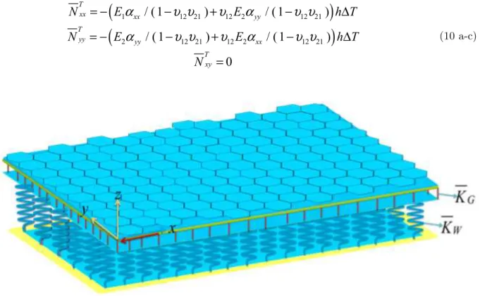
is set to zero. A mono-layered rectangular graphene sheetem-bedded in an elastic medium (polymer matrix) is shown in Figure 1. A Pasternak-type foundation model is considered for simulating the elastic medium (polymer matrix) which accounts for both normal pressure and the transverse shear deformation of the surrounding elastic medium. The vibration equation for the orthotropic rectangular nanoplates is expressed as
2 2
2 2 2 2
2 2 2 2
2 2 2 4 4
0 2
2 2 2 2 2 2 2
2
xy yy T T2
Txx
xx yy xy
W Gx Gy
M
M
M
w
w
w
f
N
N
N
x
x y
y
x
y
x y
w
w
w
w
w
K W
K
K
I
I
x
y
t
x t
y t
∂
∂
∂
∂
∂
∂
+
+
+
+
+
+
∂
∂ ∂
∂
∂
∂
∂ ∂
⎛
⎞
∂
∂
∂
∂
∂
−
+
+
=
−
⎜
+
⎟
∂
∂
∂
⎝
∂ ∂
∂ ∂
⎠
(8)where
K
W denote the Winkler modulus,K
Gx andK
Gy are the shear modulus of thesurround-ing elastic medium. If polymer matrix is homogeneous and isotropic, we will get
Gx Gy G
K
=
K
=
K
. If the shear layer foundation stiffness is neglected, Pasternak foundation tends to Winkler foundation. The termf
indicate transverse loading,I
0 andI
2 are mass moments of inertia that are defined as follows2 2
2
0 2
2 2
, I
h h
h h
I
ρ
dz
ρ
z dz
− −
=
∫
=
∫
(9)where
ρ
indicates the density of the graphene sheets. Also resultant thermal stresses(i, j= x, y)
T ij
Latin American Journal of Solids and Structures 11 (2014) 437 - 458
(
1/ ( 1
12 21)
12 2/ ( 1
12 21)
)
T
xx xx yy
N
=
−
E
α
−
υ υ
+
υ
E
α
−
υ υ
h T
Δ
(
2/ ( 1
12 21)
12 2/ ( 1
12 21)
)
T
yy yy xx
N
=
−
E
α
−
υ υ
+
υ
E
α
−
υ υ
h T
Δ
0
T xy
N
=
(10 a-c)
Figure 1 rectangular nanoplate embedded in an elastic medium
So we have Using Equations (6) and (8) we have the following governing equation in terms of the lateral deflection
(
)
(
)
4 4 4
11 4 12 66 2 2 22 4
2 2 2 4 4
0 2
2 2 2 2 2 2 2
2 2
0
2 2
2 2
2 2 2 4 4
0 2
2 2 2 2 2 2 2
2
2
T T
xx yy
i
W Gx Gy
T T
xx yy
w
w
w
D
D
D
D
x
x y
y
w
w
w
w
w
f
N
N
I
I
x
y
t
t x
t y
e l
w
w
K W
K
K
x
y
w
w
w
w
w
f
N
N
I
I
x
y
t
t x
t y
∂
∂
∂
+
+
+
∂
∂ ∂
∂
⎛
∂
∂
∂
⎛
∂
∂
⎞
⎞
+
+
−
+
+
⎜
∂
∂
∂
⎜
∂ ∂
∂ ∂
⎟
⎟
⎝
⎠
⎜
⎟
+
∇ ⎜
⎟
∂
∂
⎜
−
+
+
⎟
⎜
∂
∂
⎟
⎝
⎠
⎛
∂
∂
∂
∂
∂
+
+
−
+
+
∂
∂
∂
∂ ∂
∂ ∂
−
2 2
2 2
0.
W Gx Gy
w
w
K W
K
K
x
y
⎛
⎞
⎞
⎜
⎜
⎟
⎟
⎝
⎠
⎜
⎟
=
⎜
∂
∂
⎟
⎜
−
+
+
⎟
⎜
∂
∂
⎟
⎝
⎠
(11)
Latin American Journal of Solids and Structures 11 (2014) 437 - 458 (2004) investigated micro-continuum field theories such as couple stress theory, micromorphic theory, nonlocal theory, Cosserat theory from the atomistic viewpoint of lattice dynamics and molecular dynamics (MD) simulations. It is reported in their work that the nonlocal elasticity theory is physically reasonable.
3 SO LU T IO N P R O C E D U R E S
It is assumed that the nanoplate is free from transverse loadings
(
f
=
0
)
. Exact solution of Equation (11) can be developed for some particular boundary conditions. In this article, initially, by using the Navier’s approach orthotropic nanoplate problem is solved with simply supported boundary conditions. Then Levy type solution is used for orthotropic nanoplates, that at least for opposite edges, is simply supported.3.1 Solution using N avier’s approach
For simply supported boundary conditions, the shape function can be given by double Fourier series (Aksencer and Aydogdu, 2011)
1 1
( , , )
mnsin(
) sin(
)
i tm n
m x
n y
w x y t
W
e
a
b
ω
π
π
∞ ∞
= =
=
∑∑
(12)where m and n are the half wave numbers. Substituting from Equation (12) into Equation (11) yields the nondimensional natural frequency at small scale with various nanoplate properties, Winkler and shear elastic factors and resultant thermal stresses.
(
)
(
)
(
)
(
)
(
)
(
)
4 2 2 4
11 12 66 22
2 4 2 2 2 4 2 2
0 0
2 2 2 2 4 2 2
0 0
2 4 2 2
0
(
)
2
2
(
) (
)
(
)
(
)
(
) (
)
(
)
(
) (
)
(
)
(
)
(
)
(
) (
)
(
)
(
) (
)
T T xx yy i i W Gx i i Gy im
m
n
n
D
D
D
D
a
a
b
b
m
m
n
n
m
n
e l
N
e l
N
a
a
b
b
a
b
m
n
m
m
n
e l
K
e l
K
a
b
a
a
b
n
m
n
e l
K
b
a
b
π
π
π
π
π
π
π
π
π
π
π
π
π
π
π
π
π
π
+
+
+
⎛
⎞
⎛
⎞
+
⎜
+
⎟
+
⎜
+
⎟
⎝
⎠
⎝
⎠
⎛
⎞
⎛
⎞
+
⎜
+
⎟
+
⎜
+
⎟
⎝
⎠
⎝
⎠
+
+
(
)
(
)
2 22 2 2 2 2 2
0 2
2 2 2 2 2 4 2 2 4
0 0 2 0
(
)
(
)
(
)
(
)
(
)
(
)
(
)
(
)
(
)
2(
) (
)
(
)
0.
T T
xx yy
W Gx Gy
i i
m
n
N
N
a
b
m
n
m
n
K
K
K
I
I
a
b
a
b
m
n
m
m
n
n
I
e l
I
e l
a
b
a
a
b
b
π
π
π
π
ω
ω
π
π
π
π
π
π
π
π
ω
⎛
⎞
+
+
⎜
⎟
⎝
⎠
⎛
⎞
+
+
+
−
−
⎜
+
⎟
⎝
⎠
⎛
⎞
⎛
⎞
−
⎜
+
⎟
−
⎜
+
+
⎟
=
⎝
⎠
⎝
⎠
(13)With multiply Equation (13) in 4 11
Latin American Journal of Solids and Structures 11 (2014) 437 - 458
(
)
(
)
(
)
(
)
(
(
)
)
(
)
(
)
(
(
)
)
(
)
(
)
(
)
4 2 2 2 4 4 4 2 2 6 4 4 2 2
1 2
2 2 4 2 2 2 2 2 4 2 2 2
2 2 2 4 4 2 2 2 2 2 2 2
2 4 2 4 2 2
2 0 2 2 2 0 2 2 4 2 2 2 4 4
11 11 11
2 2
2 2 2
2 11
2
1
2
0.
Gy T Gx xx T yy WK
K
N
N
K
I
a
I
a
I
a
D
D
D
I
a
D
α
λ κ α β
λ κ β
κ β
µ
κ β
κ α β
α
µ
α
κ α β
α
µ
α
κ α β
κ β
µ
κ β
κ α β
µ
α
κ β
ω
ω
ω
µ
α
κ β
µ
α
κ β α
κ β
ω
α
κ β
+
+
+
+
+
+
+
+
+
+
+
+
+
+
+
+
+
−
+
−
−
+
+
−
+
=
(14)From Equation (9) we have
3
0
,
212
h
I
=
ρ
h I
=
ρ
(15)where nondimensional frequency parameter and other terms are defined in the following form
2 0 12 66
1
11 11
4 2 2 2 2
22 2
11 11 11 11 11 11
3
2 2 4 2 2 2 2
0 2
11 11
2
,
,
, = n ,
,
,
,
12
,K
, K
, K
,
,
,
12
iT T
W Gx Gy T xx T yy
W Gx Gy xx yy
e l
D
D
h
a
h
a
m
D
a
b
a
D
D
K a
K a
K b
N a
N a
N
N
D
D
D
D
D
D
h
h
I
a
I
a
D
D
ρ
ω
µ
α
π β
π κ
ε
λ
λ
ρ
ρ
ω
ε
ω
+
Ω
=
=
=
=
=
=
=
=
=
=
=
=
=
Ω
=
=
Ω
=
(16)
With Substituting Equation (15) in Equation (14) we have
(
)
(
)
(
)
(
)
(
(
)
)
(
)
(
)
(
(
)
)
(
)
(
)
(
)
4 2 2 2 4 4 4 2 2 6 4 4 2 2
1 2
2 2 4 2 2 2 2 2 4 2 2 2
2 2 2 4 4 2 2 2 2 2 2 2
2 4 2 4 3 2 4
2 2 2 2 2 4 2 2 2 4 4
2
11 11 11
3 2 4
2 2 2 2 11
2
1
2
12
0
12
Gy T Gx xx T yy WK
K
N
N
K
h
a
h
a
h
a
D
D
a D
h
a
a D
α
λ κ α β
λ κ β
κ β
µ
κ β
κ α β
α
µ
α
κ α β
α
µ
α
κ α β
κ β
µ
κ β
κ α β
µ
α
κ β
ρ ω
ρ ω
ρ ω
µ
α
κ β
µ
α
κ β α
κ β
ρ ω
α
κ β
Latin American Journal of Solids and Structures 11 (2014) 437 - 458 Substituting 2
(
)
2 40 11
I
=
Ω
=
ρ
h D
ω
a
andI
2=
Ω
2ε
2=
(
ρ
h
312
D
11)
ω
2a
2 in Equation(17) leads to
(
)
(
)
(
)
(
)
(
(
)
)
(
)
(
)
(
(
)
)
(
)
(
)
(
)
4 2 2 2 4 4 4 2 2 6 4 4 2 2
1 2
2 2 4 2 2 2 2 2 4 2 2 2
2 2 2 4 4 2 2 2 2 2 2 2
2 2 2 2 2 4 2 2 2 4 4
0 0 2
2 2 2
2
2
1
2
0.
Gy
T
Gx xx
T
yy W
K
K
N
N
K
I
I
I
I
α
λ κ α β
λ κ β
κ β
µ
κ β
κ α β
α
µ
α
κ α β
α
µ
α
κ α β
κ β
µ
κ β
κ α β
µ
α
κ β
µ
α
κ β
µ
α
κ β α
κ β
α
κ β
+
+
+
+
+
+
+
+
+
+
+
+
+
+
+
+
+
−
+
−
−
+
+
−
+
=
(18)
By arranging Equation (18) in term of 2
Ω
leads to
Ω
2=
α
4+
2
λ1
κ
2α
2β
2+
λ2κ
4β
4+
K
Gy
κ
4
β
2+
µ
2(
κ
6β
4+κ
4α
2β
2)
(
)
+
K
Gx(
α
2+
µ
2(
α
4+
κ
2α
2β
2)
)
+
N
xxT(
α
2+
µ
2(
α
4+κ
2α
2β
2)
)
+
N
yyT(
κ
2β
2+
µ
2(
κ
4β
4+κ
2α
2β
2)
)
+
K
W(
µ
2(
α
2+
κ
2β
2)
+
1
)
⎛
⎝
⎜
⎜
⎜
⎜
⎞
⎠
⎟
⎟
⎟
⎟
α
2+
κ
2β
2(
)
ε
2+
µ
2(
ε
2(
α
2+κ
2β
2)
+
1
)
(
)
+
1
(19)
3.2 Solution using Levy type
To solve Equation (11) for a rectangular nanoplate with arbitrary boundary conditions, Levy’s type of solution can be applied to nanoplates that are simply supported at two opposite edges. Assuming that the simple supports are at x = 0 and x = a, the shape function takes the form as (Aksencer and Aydogdu, 2011):
1
( , , )
( ) ( )
i t( ) sin
i tm
m x
w x y t
X x Y y e
Y y
e
a
ω ∞
π
ω=
⎛
⎞
=
=
⎜
⎟
⎝
⎠
∑
(20)Substituting of Equation (20) into Equation (11) leads to ( 4 ) ( 2 )
2
0
Y
−
BY
+
C
=
(21)Latin American Journal of Solids and Structures 11 (2014) 437 - 458
B
=
2
λ1
κ
2α
2+
K
Gyµ
2
κ
4α
2+
κ
4(
)
+
K
Wµ
2κ
2+
K
Gxµ
2κ
2α
2+
N
yyT(
µ
2κ
2α
2+κ
2)
+
N
xxTµ
2κ
2α
2− Ω
2(
µ
2κ
2+
2
µ
2κ
2α
2ε
2+κ
2ε
2)
⎛
⎝
⎜
⎜
⎞
⎠
⎟
⎟
2
λ2
κ
4+
µ
2K
Gyκ
6
− Ω
2µ
2ε
2κ
4+
N
yyTµ
2κ
4(
)
(22)
C
=
K
Wµ
2α
2+
1
(
)
+
K
Gxµ
2α
4+
α
2(
)
+
α
4+
N
xxTµ
2α
4+
α
2(
)
−Ω
2µ
2α
2+
µ
2α
4ε
2+
α
2ε
2+
1
(
)
⎛
⎝
⎜
⎜
⎞
⎠
⎟
⎟
λ
2κ
4
+
µ
2K
Gyκ
6− Ω
2µ
2ε
2κ
4+
N
yyTµ
2κ
4(
)
(23)
Substituting
Y y
( )
=
e
sy into Equation (21)4 2
2
0
S
−
BS
+
C
=
(24)Hence, for the orthotropic rectangular nanoplate, using the Levy-type solution requires four different forms of solution of
Y y
(
)
to be put in Equation (20) depending on the relative rigidity of the nanoplate in various directions, Winkler elastic and shear elastic factor, nonlocal parameter and thermal change. the roots in the form as followsFor the case 2
0
<
C
<
B
The general solution for
Y y
(
)
is found to be1 1 2 1 3 2 4 2
( )
sinh(
)
cosh(
)
sinh(
)
cosh(
)
Y y
=
C
δ
y
+
C
δ
y
+
C
δ
y
+
C
δ
y
(25)where
2 2
1
B
B
C
,
2B
B
C
δ
=
+
−
δ
=
−
−
(26)For the case
B
2C
=
* * * *
1 2 3 3 4 3
( )
(
) cosh(
) (
) sinh(
)
Y y
=
C
+
C y
δ
y
+
C
+
C y
δ
y
(27)where the roots are
( )
1 23
B
Latin American Journal of Solids and Structures 11 (2014) 437 - 458 For the case
C
B
2>
** **
1 5 2 5 4
** **
3 5 4 5 4
( ) (
cos(
)
sin(
))cosh(
)
(
cos(
)
sin(
)) sinh(
)
Y y
C
y
C
y
y
C
y
C
y
y
δ
δ
δ
δ
δ
δ
=
+
+
+
(29)where the roots are
1 2 1 2
4 5
1
1
,
2
2
C
B
C
B
δ
=
⎛
⎜
⎡
⎣
+
⎦
⎤
⎟
⎞
δ
=
⎛
⎜
⎡
⎣
−
⎤
⎦
⎞
⎟
⎝
⎠
⎝
⎠
(30)For the case
C
<
0
*** *** *** ***
1 6 2 6 3 7 4 7
( )
sin(
)
cos(
)
sinh(
)
cosh(
)
Y y
=
C
δ
y
+
C
δ
y
+
C
δ
y
+
C
δ
y
(31)where the roots are
2 2
6
B
C
B
,
7B
C
B
δ
=
−
−
δ
=
−
+
(32)Obviously, for a given nanoplate whose nonlaocal parameter, shear and Winkler elastic factors and other parameters have been specified only one of the four case needs to be solves to obtain frequency equations. The constants (
C
i,
C
*j,
C C
**k,
l***(i,j,k,l=1,2,3,4)
) are determined from the boundary conditions aty
=
0
andy
=
b
. The boundary conditions yield the frequency equa-tion from which ω is determined. The procedure is shown below for three states boundary condi-tions and for caseC
<
0
the procedure for other cases is similar. The boundary conditions forsimply supported edges, for instance, are
2 2
2 2
0
Y(0)=Y(b)=
0
y y b
d Y
d Y
dy
==
dy
==
(33)Using Equation (31), the boundary conditions of Equation (33) can be expressed as *** ***
2 4
0
C
+
C
=
2 *** 2 ***
6
C
2 7C
40
δ
−
δ
=
*** *** *** ***
1
sin(
6)
2cos(
6)
3sinh(
7)
4cosh(
7) 0
C
δ
b
+
C
δ
b
+
C
δ
b
+
C
δ
b
=
*** 2 *** 2 *** 2 *** 2
1 6
sin(
6)
2 6cos(
6)
3 7sinh(
7)
4 7cosh(
7) 0
C
δ
δ
b
+
C
δ
δ
b
−
C
δ
δ
b
−
C
δ
δ
b
=
Latin American Journal of Solids and Structures 11 (2014) 437 - 458 Equations (34a, b) yield
*** ***
2 4
0
C
=
C
=
(35)Equations (34c, d) can be written in matrix form as ***
6 7 1
2 2 ***
6 6 7 7 3
sin(
) sinh(
)
0
sin(
)
sinh(
)
b
b
C
b
b
C
δ
δ
δ
δ
δ
δ
⎧
⎫
⎡
⎤
=
⎨
⎬
⎢
−
⎥
⎣
⎦ ⎩
⎭
(36)For a nontrivial solution, we should have
sin(
δ
6b
) 0
=
or6
n
b
.
δ
=
π
When edgey
=
0
andy
=
b
are clamped. The boundary conditions can be stated as0
Y(0)= Y(b)=
0
y y b
dY
dY
dy
==
dy
==
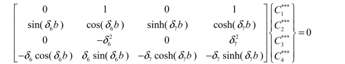
(37)By inserting Equation (31) into Equation (37), the boundary conditions can be written in ma-trix form as
*** 1 ***
6 6 7 7 2
***
6 7 3
***
6 6 6 6 7 7 7 7 4
0
1
0
1
sin(
)
cos(
)
sinh(
)
cosh(
)
0
0
0
cos(
)
sin(
)
cosh(
)
sinh(
)
C
b
b
b
b
C
C
b
b
b
b
C
δ
δ
δ
δ
δ
δ
δ
δ
δ
δ
δ
δ
δ
δ
⎧
⎫
⎡
⎤
⎪
⎪
⎢
⎥
⎪
⎪
⎢
⎥
⎨
⎬
=
⎢
⎥ ⎪
⎪
⎢
⎥ ⎪
⎪
−
−
−
⎣
⎦ ⎩
⎭
(38)
By setting the determinant of the matrix in Equation (38) equal to zero, we obtain the fre-quency characteristic equation.
(
)
(
2 2)
6 7 6 7 7 6 6 7
2
δ δ
cos(
δ
b
)cosh(
δ
b
) 1
−
−
δ
−
δ
sin(
δ
b
)sinh(
δ
b
) 0
=
(39) When the one edge of the rectangular nanoplate is clamped and other edge is simple support-ed, the additional four boundary conditions are2
2 0
Y(0)=Y(b)=
0
y b y
d Y
dY
dy
dy
==
=
=
(40)Latin American Journal of Solids and Structures 11 (2014) 437 - 458
*** 1 ***
6 6 7 7 2
2 2 ***
6 7 3
***
6 6 6 6 7 7 7 7 4
0
1
0
1
sin(
)
cos(
)
sinh(
)
cosh(
)
0
0
0
cos(
)
sin(
)
cosh(
)
sinh(
)
C
b
b
b
b
C
C
b
b
b
b
C
δ
δ
δ
δ
δ
δ
δ
δ
δ
δ
δ
δ
δ
δ
⎧
⎫
⎡
⎤
⎪
⎪
⎢
⎥
⎪
⎪
⎢
⎥
⎨
⎬
=
⎢
−
⎥
⎪
⎪
⎢
⎥ ⎪
⎪
−
−
−
⎣
⎦ ⎩
⎭
(41)
A nontrivial solution can be obtained by equating the determinant of these equations to zero. Consequently, we have
7
cosh(
7b
)sin(
6b
)
6sinh(
7b
)cos(
6b
) 0
δ
δ
δ
−
δ
δ
δ
=
(42)For any specific value of m, there will be successive value of
Ω
. The natural frequencies can be denote asω
11,
ω
12,
ω
13, ...,
ω
21,
ω
22, ...,
whose value depend on the material properties1 2 12 12
E , E ,
υ
,
υ
, ,
ρ α
xx,
α
yy and geometryh
,
a b
and nonlocal parameter of the rectangular nanoplate. The frequency characteristic equations and the mode shapes for other case can be de-rived in a similar manner. The results for the three combinations of boundary conditions are summarized in Table 1. According to Table 1, by insertingY y
(
)
into Equation (20) we have mode shape for orthotropic rectangular nanoplates based on elastic medium for different bounda-ry conditions. Following three boundabounda-ry conditions have been investigated in the vibration analy-sis of the rectangular graphene sheets as: SSSS, SCSC and SSSC that refer to Appendix 7.2 for more detail.Table 1 Frequency equation and mode shape orthotropic rectangular nanoplates with different boundary conditions
Boundary conditions
Type Equation
SSSS Mode shape
(
)
Y y
sin(
β
ny)
β
n=
n
π
b
SCSC Mode shape
(
)
Y y
(
)(
)
(
)(
)
7 6 6 7 7 6
6 7 7 6 7 6
cosh(
) cos(
)
sinh(
)
sin(
)
sinh(
)
sin(
) cosh(
) cos(
)
b
b
y
y
b
b
y
y
δ
δ
δ
δ
δ
δ
δ
δ
δ
δ
δ
δ
−
−
⎧
⎫
⎪
⎪
⎨
⎬
−
−
−
⎪
⎪
⎩
⎭
SSSC Mode shape
(
)
Y y
sin(
δ
6b
)sinh(
δ
7y
) sinh(
−
δ
7b
)sin(
δ
6y
)
Latin American Journal of Solids and Structures 11 (2014) 437 - 458 4 R ESU LT S A N D D ISC U SSIO N
4.1 V alidation of present results
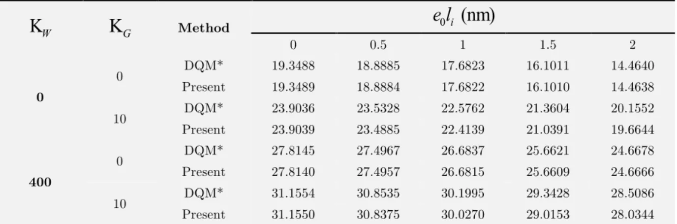
To validate the results, comparison of the present results for orthotropic rectangular nanoplate embedded in an elastic medium with the obtained results by DQM (Pradhan and Kumar 2010) is studied. In the present study non-dimensional frequency are calculated for all edges Simply Sup-ported boundary conditions, these results are listed in Table 2.
Table 2 Comparison of results for vibration of the graphene sheet for all edges simply supported. (* (Pradhan and Kumar 2010)).
K
WK
G Method0 i
(nm)
e l
0 0.5 1 1.5 2
0
0 DQM* 19.3488 18.8885 17.6823 16.1011 14.4640
Present 19.3489 18.8884 17.6822 16.1010 14.4638
10 DQM* 23.9036 23.5328 22.5762 21.3604 20.1552
Present 23.9039 23.4885 22.4139 21.0391 19.6644
400
0 DQM* 27.8145 27.4967 26.6837 25.6621 24.6678
Present 27.8140 27.4957 26.6815 25.6609 24.6666
10 DQM* 31.1554 30.8535 30.1995 29.3428 28.5086
Present 31.1550 30.8375 30.0270 29.0153 28.0344
From this table one could find that the present results for the nanoplate exactly match with those reported by Pradhan and Kumar (2010). The scale coefficients are assumed as
0i
0.0, 0.5, 1.0, 1.5,
e l
=
and2.0 nm
, respectively. The value of nonlocal parameter is taken in the range of 0–2 nm. Duan and Wang (2007) presented the constitutive relations of nonlocal elas-ticity theory for application in the analysis of circular graphene sheet. Recently, these values for the nonlocal parameter are used by many researchers (Farajpour et al 2011b; Danesh et al. 2012; Farajpour et al 2012; Mohammadi et al. 2013b). Properties of the orthotropic graphene sheet in this paper are considered same as mentioned in the reference (Liew et al 2006).3 1
1765 Gpa,
21588 Gpa,
120.3,
210.27 , = 2300
,
E
=
E
=
υ
=
υ
=
ρ
kg m
The material properties for isotropic graphene sheet are taken from Ref. (Liew et al 2006). 3
1
,
21060 Gpa, = 2250
,
12 210.25
E E
=
ρ
kg m
υ
=
υ
=
.The coefficients of thermal expansion are considered for orthotropic graphene sheet
3
yy xx
α
=
α
from Ref. (Malekzadeh et al 2011) and for isotropic graphene sheet are taken xx yyα
=
α
. For the room or low temperature case thermal coefficient is taken( 6 ) 1
1.6 10
K
xx
α
− −=
−
×
and for high temperature case that is considered ( 6 ) 11.1 10
K
xxα
− −=
×
.These values were used for carbon nanotube (Zhang et al. 2007).
Latin American Journal of Solids and Structures 11 (2014) 437 - 458 condition. In this table, the Winkler factor and shear factor are ignored. These results are exactly in agreement with that presented by Pradhan and Kumar (2011).
Table 3 Comparison of results for vibration of the orthotropic graphene sheet for two set boundary conditions. (** (Pradhan and Kumar 2011)).
Method
e l
0 i(nm)
0 0.5 1 1.5 2
SCSS boundary conditions
DQM** 22.9849 22.4022 20.8867 18.9234 16.9171
Present 22.9849 22.4021 20.8865 18.9230 16.9166
SCSC boundary conditions
DQM** 27.9208 27.1853 25.2818 22.8350 20.3555
Present 27.9207 27.1851 25.2813 22.8341 20.3543
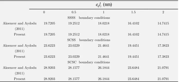
For further validations, we compared the results of rectangular nanoplates with published data. As shown in Table 4 results of Aksencer and Aydogdu (2011), compared to results obtained by present work for isotropic rectangular nanoplates without consider effect of elastic medium and thermal effect. These results are exactly in agreement with that presented by Aksencer and Ay-dogdu (2011).
Table 4 Comparison of results for vibration of the isotropic graphene sheet for three set boundary conditions.
0i
(nm)
e l
0 0.5 1 1.5 2
SSSS boundary conditions Aksencer and Aydodu
(2011)
19.7205 19.2512 18.0218 16.4102 14.7415
Present 19.7205 19.2512 18.0218 16.4102 14.7415
SCSS boundary conditions Aksencer and Aydodu
(2011)
23.6223 23.0229 21.4641 19.4451 17.3823
Present 23.6223 23.0229 21.4641 19.4451 17.3823
SCSC boundary conditions Aksencer and Aydodu
(2011)
28.9203 28.1577 26.1844 23.6484 21.0791
Latin American Journal of Solids and Structures 11 (2014) 437 - 458
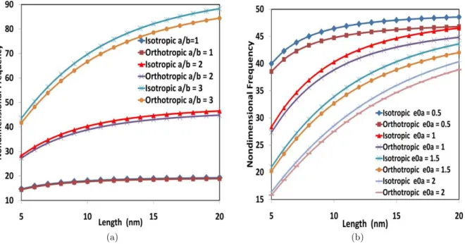
(a) (b)
Figure 2 Change non-dimensional frequency with length of orthotropic and isotropic rectangular nanoplate for SSSS boundary condi-tion and e0li=1 nm (a) various aspect ratios (b) various nonlocal parameters (a/b=2).
4.2 Length effects on the frequency of orthotropic graphene sheet
Latin American Journal of Solids and Structures 11 (2014) 437 - 458
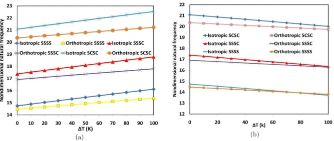
(a) (b)
Figure 3 Change non-dimensional frequency with temperature change for various boundary conditions and isotropic and orthotropic graphene sheet in the case of (a) low temperature (b) high temperature. (a/b= 1, eoli=2 nm)
4.3 Effects of tem perature case on the frequency of orthotropic graphene sheet
To study the influence of low and high temperature case on the vibration characteristics of rec-tangular nanoplates, the variation in non-dimensional natural frequency with the temperature change is shown in Figure 3. The curves are plotted for isotropic and orthotropic properties, first mode numbers and three cases boundary condition. The length of the square nanoplate, the local parameter and aspect ratio are considered 10 nm, 2 nm and 1 respectively. It is shown non-dimensional frequency of the isotropic small-sized graphene sheet is always larger than that of orthotropic one for case of low temperature in Figure 3a. Furthermore, the gap between the two curves (isotropic and orthotropic) increases with an increase in temperature changes. In other words, the difference between the natural frequencies calculated by isotropic and orthotropic properties decreases with decreasing temperature change. Moreover, for this case the non-dimensional frequency increases with increase the temperature change. The temperature change is important for graphene sheet with isotropic properties because the slope of curve isotropic is more than orthotropic curves. Also, it is seen from this results that the nondimensional natural fre-quency for SCSC boundary condition is higher than that for SSSC and SSSS at low temperature case.
iso-Latin American Journal of Solids and Structures 11 (2014) 437 - 458
tropic properties. The phenomenon could be attributed to the fact that the coefficient of thermal expansion in case of orthotropic graphene sheet in compared with the isotropic grapheme sheet are much less in the “Y” direction. Also, it is seen from this results the non-dimensional natural frequency for SCSC boundary condition is higher than the non-dimensional natural frequency for SSSC and SSSS boundary conditions at high temperature case.
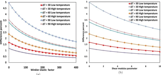
(a) (b)
Figure 4 Variation of difference percent for various temperature changes of graphene sheet and low and high temperature case. (a) Shear modulus parameter (b) Winkler elastic factor. (SSSS boundary condition, a=10 nm, a/b=1, eoli= 2 nm)
4.4 Elastic m edium effects on natural frequency of orthotropic graphene sheet
The effect of temperature change on the frequency of orthotropic graphene sheet embedded in an elastic medium is studied. The Winkler modulus parameter
K
W, for the surrounding polymer ma-trix is gotten in the range of 0–400. We assumed that polymer mama-trix is homogeneousGx Gy G
K
=
K
=
K
. Then shear modulus factorK
G is gotten in the range 0-10. Similar values ofmodulus parameter were taken by Liew et al. (2006). The relationships between frequency differ-ence percent versus Winkler constant
K
W and shear modulusK
G for different temperaturechanges and low and high temperature case are demonstrated in Figures 4a, b. A scale coefficient e0a = 2.0 nm is used in the analysis. In this figure boundary condition, length of nanoplate and aspect ratio are assumed SSSS, 10 nm and 1 respectively. The frequency difference percent is defined as
( ) 0
0
Difference percent=
T T K T100
T
frequency
frequency
frequency
Δ = Δ =
Δ =
−
Latin American Journal of Solids and Structures 11 (2014) 437 - 458 As can be seen, the Winkler constant or shear modulus decreases then the effect of thermal on the difference percent increases. It can be seen from the results that the difference percent in-creases with increasing the temperature change. For larger temperature change, the decline of difference percent is quite important. Also, the difference percent for low temperature case is larger than that for case of high temperature. Furthermore the decline for the high temperature case is much less than that for case of low temperature. From these plots obvious the important influence of temperature change, in the cases low and high temperature case on the non-dimensional frequency of embedded orthotropic graphene sheet.
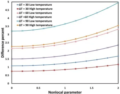
4.5 N onlocal effects on natural frequency of orthotropic graphene sheet
Figure 5 shows the frequency difference percent with respect to nonlocal parameter. In this inves-tigation we consider SSSS boundary condition, a=10 nm and a/b=1. It is seen that the frequency difference percent increases with the increase of the temperature change. Also, the results show that the difference percent increases monotonically by increasing the nonlocal parameter. In other words, that nonlocal solution for difference percent is larger than the local solutions. In Figures 4a, b, and 5, the gap between low and high temperature cases increases with increasing the tem-perature change.
Latin American Journal of Solids and Structures 11 (2014) 437 - 458 5 C O N C LU SIO N S
In this study, using the nonlocal elasticity continuum plate model, the effects of the temperature change on the vibration frequency of orthotropic and isotropic rectangular nanoplate embedded in an elastic medium was investigated for two cases low and high temperature. The elastic medium based on the Pasternak foundation was taken general case (the polymer matrix was considered non-homogeneous). Nonlocal elasticity theory has been applied to capture the structural discrete-ness of small-size plates (nanoplates). Equation of motion based on nonlocal theory has been de-rived. Exact closed form solutions for the free vibration nanoscale rectangular nanoplates are ob-tained using Navier's and Levy type solutions. Results for three set boundary condition are pre-sented by levy type solution. From the results following conclusions are observed
• Small-scale effect has an increasing effect on the non-dimensional natural frequency of or-thotropic and isotropic rectangular nanoplate. Scale effect is less prominent in lager length of nanoplate.
• The difference between the natural frequencies calculated by isotropic and orthotropic properties increases with increasing aspect ratio and length of nanoplate.
• The non-dimensional frequency is larger for higher aspect ratio and length of rectangular nanoplate.
• The non-dimensional natural frequency decreases at high temperature case with increasing the temperature change for all boundary conditions of isotropic and orthotropic rectangu-lar graphene sheet.
• The effect of temperature change on the non-dimensional frequency vibration becomes the opposite at low temperature case in compression with the high temperature case.
• when Winkler or elastic factors increases, the frequency difference percent decreases at low and high temperature cases.
• The difference percent increases monotonically by increasing the nonlocal parameter. • The difference between low and high temperature cases increases with increasing the
tem-perature change. References
Akgöz B., Civalek Ö. (2011a).Application of strain gradient elasticity theory for buckling analysis of protein microtubules. Current Applied Physics 11: 1133-1138.
Akgöz B., Civalek Ö. (2011b). Strain gradiant and modified couple stress models for buckling analysis of axial-ly loaded micro-scales beam. International Journal of Engineering Science 49: 1268-1280.
Akgöz B., Civalek Ö. (2012a).Analysis of micro-sized beams for various boundary conditions based on the strain gradient elasticity theory. Archive of Applied Mechanics 82: 423-443.
Akgöz B., Civalek Ö. (2012b). Free vibration analysis for single-layered graphene sheets in an elastic matrix via modified couple stress theory. Materials & Design 42: 164-171.
Akgöz B., Civalek Ö. (2013a). A size-dependent shear deformation beam model based on the strain gradient elasticity theory. International Journal of Engineering Science 70: 1-14.
Akgöz B., Civalek Ö. (2013b). Modeling and analysis of micro-sized plates resting on elastic medium using the modified couple stress theory. Meccanica 48: 863-873.