Gustavo Bono
[email protected] Federal University of Rio Grande do Sul - UFRGS Graduate Program in Mechanical Engineering 90050-170, Porto Alegre, RS, Brazil
Armando Miguel Awruch
Senior Member, ABCM [email protected] Federal University of Rio Grande do Sul - UFRGS Applied and Computational Mechanical Center 90035-190, Porto Alegre, RS, Brazil
An Adaptive Mesh Strategy for High
Compressible Flows Based on Nodal
Re-Allocation
An adaptive mesh strategy based on nodal re-allocation is presented in this work. This technique is applied to problems involving compressible flows with strong shocks waves, improving the accuracy and efficiency of the numerical solution. The initial mesh is continuously adapted during the solution process keeping, as much as possible, mesh smoothness and local orthogonality using an unconstrained nonlinear optimization method. The adaptive procedure, which is coupled to an edge-based error estimate aiming to equidistribute the error over the cell edges is the main contribution of this work. The flow is simulated using the Finite Element Method (FEM) with an explicit one-step Taylor-Galerkin scheme, in which an Arbitrary Lagrangean-Eulerian (ALE) description is employed to take into account mesh movement. Finally, to demonstrate the capabilities of the adaptive process, several examples of compressible inviscid flows are presented. Keywords: adaptive mesh strategy,high compressible flows,finite element method
Introduction
1
The numerical solution of complex problems in many engineering fields normally requires the use of a large number of mesh points to accurately capture phenomena exhibiting high gradients of one or more variables such as those appearing in boundary layers, regions with stress concentrations, shock waves, etc. As the regions where these phenomena take place are not
known a priori in most cases, it is rarely feasible to create a suitable
initial mesh with small elements at the corresponding location, where high gradients may be found.
Several approaches have been employed for both structured and unstructured mesh adaptation. The most widely used approaches consist in nodal re-allocation, automatic mesh refinement/unrefinement and changes of the approximation order of the variables. Sometimes it is appropriate to use simultaneously more than one of these approaches. Most of these subjects are well summarized in Löhner (2001), where many references are given.
A strategy for mesh adaption, using only mesh movement and nodal re-allocation, has the advantage that the mesh connectivity and number of elements and nodes do not vary with respect to the initial mesh and hence computational cost does not increase when a new flowfield is calculated on the adapted mesh. This intrinsic
simplicity is also the cause of the limitations of r-strategy. The
accuracy which can be achieved with an adaptive mesh nodal re-allocation strategy is limited, because the number of nodes and the mesh topology are fixed from the beginning, when the initial mesh is built. In fact, the initial mesh heavily influences the adaptive process. Once the node location is “optimal” according to the error estimate, a more accurate, complex and expensive solution can only be achieved by increasing the number of nodes or/and change the order of accuracy of the discretized approximation. The node movement technique, within an a posteriori adaptive framework, was originally presented by Gnoffo (1983), and was after generalized by Nakahashi and Deiwert (1987), for fluid flow problems. The schemes used by these authors are based in the spring analogy, in which the mesh is viewed as a set of springs with constraints on mesh orthogonality and their constants representing error measures. Each apex (or node) is moved until equilibrium are reached by the spring forces.
The refinement technique using exclusively nodal movement has been less popular in the finite element community; the main
Paper accepted April, 2008. Technical Editor: Olympio Achilles de F. Mello.
difficulty seems to be the lack of a reliable and general procedure to determine the mesh movement (Cao et al., 1999). Nevertheless, as this method is easy to implement and inexpensive, because only the initial mesh with a non complex data structure is needed to originate continuos changes of the mesh in the time-space domain, it is worthwhile to employ this technique whenever it is possible. This procedure may sometimes be more efficient in terms of processing time and computer memory than refinement techniques (where new nodes and elements are created).
Hawken et al. (1991) presented a review of adaptive node-movement techniques in finite elements and finite differences. Ait-Ali-Yahia et al. (1996, 1997) studied a methodology for quadrilateral elements using an edge-based error estimate with no constraints on mesh orthogonality, but high aspect ratios were obtained. However, the stability of most numerical schemes may depend on the mesh quality, for this reason, excessive mesh distortion, without any control, must be avoided using a smoothing process and preserving mesh regularity. Tam et al. (2000) extended this methodology for 3-D hexahedral and tetrahedral elements, considering nodal movement as well as the edge refinement and coarsening strategies. Hexahedral meshes have a better accuracy and require less CPU time than the tetrahedral meshes for the same number of nodes.
Nomenclature
A = area, dimensionless C = tolerance d = edge-based error D = stand-off distance e =total energy, dimensionless F = objective function
Fi = vector flux variables
h = element length H = hessian matrix
H = hessian modified matrix M = Mach number
OR = measure the local orthogonality p = thermadynamic pressure, dimensionless P = node in typical cell
r = position vector R = eigenvectors matrix s = independent variable SM = measure the local smoothness t = time, dimensionless
u = internal energy, dimensionless
U = vector of field variables
vi = fluid velocity components, dimensionless V = unit vector
wi = mesh velocity components, dimensionless Wij = monitoring function
xi = spatial coordinates, dimensionless
Greek Symbols
α = angle of attack, deg.
β = weight parameter for cell area control
δ = weight parameter for control local orthogonality and
local smoothness
δij = Kronecker delta
γ = ratio of specific heats
Λ = eigenvalues matrix
ρ = dimensionless specific mass
Subscripts
∞ freestream flow
max maximum value
min minimum value
s stagnation value
The Numerical Scheme
The governing equations for inviscid compressible flows with no source term, using an ALE description (Löhner, 2001), may be written in their dimensionless form (Bono, 2004) as:
0
i i
i i
w
t x x
∂ ∂ ∂
∂ +∂ − ∂ =
U F U
(i=1, 2,3) (1)
with, = U 1 2 3 v v v e ρ ρ ρ ρ ρ ⎧ ⎫ ⎪ ⎪ ⎪ ⎪ ⎪ ⎪ ⎨ ⎬ ⎪ ⎪ ⎪ ⎪ ⎪ ⎪ ⎩ ⎭
; Fi=
(
)
1 1 2 2 3 3 i i i i i i i i v v v p v v p v v pv e p ρ ρ δ ρ δ ρ δ ρ ⎧ ⎫ ⎪ + ⎪ ⎪ ⎪ ⎪ + ⎪ ⎨ ⎬ ⎪ + ⎪ ⎪ ⎪ + ⎪ ⎪ ⎩ ⎭ (2)
where U and Fi are vectors containing field and flux variables,
respectively. In these expressions, vi and wi are the fluid and mesh
velocity components in the direction of the spatial coordinate xi,
respectively, ρ is the specific mass, p is the thermodynamic pressure
and e is the total energy. Finally, δij is the Kronecker delta and t is
the time coordinate. Equation (1) is complemented by the equation of state for an ideal gas, which is given by:
(
1)
p= γ− ρu (3)
where γ is the ratio of specific heats at constant pressure and
volume, and u is the internal specific energy. The problem is
completely defined when initial and boundary conditions are added to these equations.
The system of partial differential equations is solved with an explicit one-step Taylor-Galerkin scheme using the finite element method (Donea, 1984; Löhner, 2001). An isoparametric eight node hexahedrical element is used and the corresponding element matrices are obtained analytically employing one-point quadrature. Integration of element matrices with uniform reduced integration may lead to the appearance of Hourglass modes, which can modify
the physical solution. To control these spurious modes the “h
-stabilization” method (Christon, 1997) was used. This code has been validated against analytical and experimental results for several compressible flows (Kessler and Awruch, 2004; Bono, 2008).
Mesh Adaptation
In general, the adaptive process with nodal redistribution consists of three main steps. The first step is to define an appropriated monitoring function, which is representative of important solution features. The second, and probably the most crucial step, is to redistribute the nodes in the computational domain in a manner which is consistent with the aforestated monitoring function. It is crucial to maintain the geometric fidelity of solid boundaries during the redistribution process. Mesh quality, measured by orthogonality and smoothness, must be also maintained. In the third step the metric terms are modified to reflect mesh movement with a consistent node speed to re-evaluate the flow variables at the new mesh using an appropriate scheme.
Monitoring Function
A key issue in this adaptive mesh strategy based on nodal re-allocation is to find a proper monitoring function to control the mesh properties and interconnect the mesh and physical solution. A
common practice consists to use the numerical solution u and/or its
derivatives (u ux, xx), so that the mesh is concentrated in regions
where the solution changes rapidly.
While it is reasonable to use the gradient of numerical solutions to identify the regions requiring high resolution, a more natural and general approach is to use error distribution since it measure directly the resolution of the numerical solution. In this work, the monitoring
function is based on the second derivative of the generical variable u
and the error is equidistributed over the edges. The specific mass is the variable used to estimate the error because the detection of shocks waves are of primary interest.
Error Estimation
Assume a one-dimensional problem, in which the specific mass
ρ is approximated by ρh using piecewise linear interpolation
2 2
2 h
d
h C
dx ρ
= (4)
where C is a specific tolerance and h is the element length. For a
three-dimensional problem, the second derivative of the specific
mass approximated by ρh with respect to a direction defined by the
versor V is given by:
2
2 T h ρ
∂ =
∂V V H V (5)
where H is the Hessian matrix. As ρh is interpolated with linear
shape functions, the second derivative of ρh at a node I can be
calculated using a weak formulation (Ait-Ali-Yahia, 1996) obtaining:
2
1 2
I I
T
T
h h h
j
j j j
j I
d n d
x x x
x
ρ − φ φ ρ φ φ ρ
Ω Γ
⎧⎡ ⎛ ⎞ ⎤⎛ ⎞ ⎛ ⎞⎫
∂ = ⎨⎪⎢− ⎜∂ ⎟ Ω⎥⎜∂ ⎟+⎡ Γ⎤⎜∂ ⎟⎪⎬
⎢ ⎥
⎜∂ ⎟ ⎜∂ ⎟ ⎣ ⎦⎜∂ ⎟ ∂ ⎪⎩⎣⎢
∫
⎝ ⎠ ⎥⎦⎝ ⎠∫
⎝ ⎠⎭⎪M (6)
where −1
M is the inverse of the mass matrix, which is given by:
(
)
11
I T
d φ φ −
− Ω
=
∫
ΩM (7)
where φ is a vector containing the shape functions, ΩI is the
volume of all the elements sharing the node I and ΓI is the
correspondign boundary. I varies from 1 until the total number of
nodes in the finite element mesh, nj represents the cossine of the
angle formed by a normal axis to ΓI with the coordinate axis xj.
The first derivatives of ρh are nodal values that can be obtained
using a smoothing process based in the mean square method. In Eq.
(6) as well as in the smoothing process to obtain values of ∂ρh ∂xj
at the nodes, the lumped mass matrix may be used instead of the consistent mass matrix, indicated in Eq. (7).
The matrix H can be diagonalized and, in this case, Eq. (5) may
be written as follows:
2
2
T T
h ρ ∂
=
∂V V RΛR V (8)
where Λ is a diagonal matrix containing the eigenvalues of H and
R contains the corresponding eigenvectors. In order to use H to
define a metric, it can be substituted by H, where the absolute
values of the eigenvalues are taken. Then, the following expression is obtained:
2
2
T T
h ρ ∂
= ≤
∂V V H V V H V (9)
where the modified Hessian matrix H is given by:
T
=R R
H Λ (10)
In Eq. (10), Λ contains the absolute values of the eigenvalues.
The criterion of mesh adaptation for a one dimensional case, taking a uniform distribution of the error over the element domain, is given by Eq. (4). Extending this concept to a 3-D case, the following equivalent equation may be written:
2
h T =C
V H V (11)
In the current approach, the error, is equidistributed over the
mesh edges, where h is the Euclidian length of an element edge, and
the second derivative of ρh is now given by Eq. (9), where V is a
unit vector that support this specific edge. An optimal mesh would be defined as the one in which all the edges have the same length
(equal to C) in the Riemann metric defined by T
V H V (see Ait-Ali-Yahia, 1996). Thus the edge-based error estimate is computed evaluating numerically the following expression on each edge:
(
)
( )
(
)
12
0 h
T h
j i j i
d = ⎡⎢ − s − ⎤⎥ ds
⎣ ⎦
∫
x x H x x (12)where xj−xi =h and s is an independent variable, such that
0≤ ≤s h.
The Mesh Movement
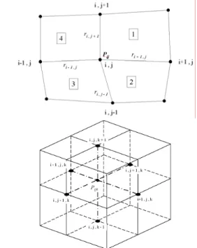
Although the formulation will be presented for two-dimensional (2-D) flows, because it is easier to understand how the algorithm works, this method was implemented to deal with three-dimensional (3-D) flows. Brackbill and Saltzman (1982) formulated the grid equations in a variational form to produce satisfactory mesh concentration while maintaining relatively good smoothness and orthogonality. In order to improve computational efficiency and reliability of this method Carcaillet et al. (1986) and Kennon and Dulikravich (1986) adopted a more heuristic formulation for the local adaptation problem. Consider a typical cell, formed by four elements in the two-dimensional case (in a 3-D case the cell would
be formed by eight elements), as it is shown in Fig. 1. Pij = P ( xij )
is a common node belonging to the four elements forming the cell, which is connected to the other nodes by straight segments defined
as position vectors ri,j.
Figure 1. Typical cells defined for two and three-dimensional cases.
The four position vectors with origin at the node Pij are used to
orthogonality, ORij, of the typical cell. The dot products are chosen
so that their sum is zero if the grid is locally orthogonal. A measure
quantifying the local smoothness, SMij, is given by the sum of the
squared values of the differences between the areas of elements forming the typical cell. The sum will be zero if all adjacent elements have the same area.
Then, local orthogonality ORij and local smoothness SMij are
given by:
(
) (
) (
)
(
)
2 2 2
1, , 1 , 1 1, 1, , 1 2
, 1 1,
ij i j i j i j i j i j i j
i j i j
OR r r r r r r
r r + + − + − − + − = ⋅ + ⋅ + ⋅ + + ⋅ (13)
(
) (
2) (
2) (
2)
21 2 2 3 3 4 4 1
ij
SM = A−A + A −A + A−A + A −A (14)
where Ak is the area of each element k forming the typical cell. The
cell area control of a typical cell is calculated with the following expression:
ij ij
W =d (15)
where Wij is a monitoring function, which gives positive values and
is evaluated at the node Pij. The choice of the weight function Wij in
the volume control is a very important aspect, because this parameter indicates where the adaptation process will take place. It
may be observed that greater values of Wij correspond to decreasing
values of the typical cell area (or volume in a 3-D case) and vice versa.
The global objective function F is obtained by a weighted linear
combination of local measures of mesh quality (local orthogonality and local smoothing) and the local volume control of a typical cell. Then, the global objective function to be minimized is given by:
(
)
1 1 max max
min min 1
I I l m ij ij ij i j OR SM F d OR SM
δ δ β
= =
⎡ ⎤
= ⎢ ⋅ + − + ⋅ ⎥
⎣ ⎦
∑∑
x x (16)
with 0≤ ≤δ 1 and 0≤ ≤β 1, where δ and β are weighting
parameters, while ORmax and SMmax are the largest values of ORij
and SMij, respectively, in order to ensure values of the same order in
Eq. (16); l and m are the number of nodes in directions i and j,
respectively. In Eq. (16), dij is obtained by the sum of the squared
values of the edge-based error-estimate h
d , given in Eq. (12), for
all the element edges having Pij as a common end. Experiences
show that β =1.0 and δ=0.5 are suitable values of the weighting
parameters. The conjugated gradient method, proposed by Fletcher-Reeves (Press et al., 1992), is used to vary the node positions until
the non-linear objective function F
{
( )
xij :1≤ ≤i l, 1≤ ≤j m}
isminimized. Restrictions are prescribed to the motion of the nodes belonging to the boundaries surfaces.
For the three-dimensional case, orthogonality and smoothness measures used by Kennon and Dulikravich (1986) were adopted. The corresponding expressions are given by the following respective expressions:
(
) (
) (
)
(
) (
) (
)
(
) (
) (
)
(
)
2 2 2
1, , , 1, , 1, 1, , 1, , , 1,
2 2 2
, 1, 1, , 1, , , , 1 , 1, , , 1
2 2 2
1, , , , 1 , 1, , , 1 1, , , , 1 2
, 1, , , 1
ijk i j k i j k i j k i j k i j k i j k i j k i j k i j k i j k i j k i j k i j k i j k i j k i j k i j k i j k i j k i j k
OR r r r r r r
r r r r r r
r r r r r r
r r r
+ + − + − − + − + − − − − − + − + + − + = ⋅ + ⋅ + ⋅ + + ⋅ + ⋅ + ⋅ + + ⋅ + ⋅ + ⋅ +
+ ⋅ +
(
) (
2)
21, , ,1, 1 , 1, , , 1
i− j k⋅ri k+ + ri j+k⋅ri j k+
(17)
(
) (
) (
)
(
) (
) (
)
1, , 1, , , 1, , 1, 1, , 1, ,
, 1, , 1, , , 1 , , 1 , , 1 , , 1 ijk i j k i j k i j k i j k i j k i j k
i j k i j k i j k i j k i j k i j k
SM r r r r r r
r r r r r r
+ + − − − −
+ + + + − −
= ⋅ + ⋅ + ⋅ +
+ ⋅ + ⋅ + ⋅ (18)
An ALE description (Löhner, 2001) was used together with the adaptive process. The velocity components of the nodes, originated by the re-allocation of a specific mesh node from its position at time
level m to a new position at m+1, are given by wi= ∆ ∆xi t
(i=1, 2,3), where ∆xi are the components of node displacement
and ∆t is the time interval.
The new nodal coordinates are updated according to the
expression, m1 m
i i i
x + =x + ∆θ x , where θ is a relaxation coefficient
which varies between 0 and 1. Boundary nodes are free to move on the corresponding boundary plane or surface.
Both, flow solver and mesh adaptation procedures, are placed in an interative loop, and the algorithm consists of the following steps:
1) Initialize the field and apply the flow solver using an initial mesh;
2) IF the adaptive process will be applied (it is an option determined by the user);
(a) - Compute H using Eq. (10);
(b) - Compute the edge-base error estimate, d, using Eq. (12)
and minimize the global objective function, given in Eq. (16); (c) - Re-allocate de nodes of the mesh and compute the mesh velocity components;
(d) - Compute the flow variables on the updated mesh using the flow solver;
3) Steps (a) to (d) is repeated NADAP times, where NADAP represents the number of application of the adaptation procedure and it is given by the user;
4) Stop if a satisfactory steady state is obtained.
Numerical Examples
For all test cases investigated here, the adaptive process was applied when the convergence criterion was reached (the tolerance
adopted for the residue of the specific mass was 10-5). The CPU
time required by the adaptive process is negligible (less than 1%).
Finally, it is assumed that γ , given in Eq. (3), is equal to 1.4.
Analytical Test Case
A simple analytical test case is used to demonstrate the effectiveness of the nodal re-allocation strategy and the relationship between the weighting parameters to improve the mesh quality in the mesh adaption process. On the unit square
{
0≤ ≤x 1.0, 0≤ ≤y 1.0}
, the monitoring function is defined as:(
) (
)
{
}
(
) (
)
{
}
(
) (
)
{
}
2 2 2 2 2 2( , ) 1000 exp 20 0.2 0.2
800 exp 50 0.6 0.7
800 exp 50 0.8 0.2
W x y x y
x y x y ⎡ ⎤ = − ⎣ − + − ⎦ + ⎡ ⎤ + − ⎣ − + − ⎦ + ⎡ ⎤ + − ⎣ − + − ⎦ + (19)
An adaptive mesh is expected to concentrate nodes around three circles. The domain is discretized using a uniform mesh with 20 x 20 x 1 elements. Figure 2 shows the relationship between the weighting parameters to obtain mesh regularity, local orthogonality and mesh adaptation employed in Eq. (16). The following values were adopted for the mesh adaptation and mesh quality parameters:
1.0 0.0
The mesh obtained with δ=0.0, Fig. 2(A), shows that the variation of the size in neighbor elements is very smooth. When
1.0
δ= , Fig. 2(C), the influence of this parameter in the mesh
orthogonality can be observed. Note that elements located in a region surrounded by the circles are highly distorted and the
smallest elements are greater than those obtained with δ=0.0. It is
interesting to note that δ=0.50 leads to a significant improvement
in the adapted mesh. As was mentioned previously, β=1.0 and
0.5
δ= are suitable values to control mesh quality.
Figure 2. Mesh for different weighting parameters (β δ). Cases: A
(1.0/0.0), B (1.0/0.5) and C (1.0/1.0).
Supersonic Flow over a Circular Cylinder
A circular half-cylinder with a dimensionless value of the radius equal to 1 is placed into a steady supersonic flow with a Mach
number equal to 3.0. The domain
{
AB=1.50,CD=3.20}
andboundary conditions of this problem are shown in Fig. 3. For this blunt-body problem a relatively coarse mesh is used, with 4
elements in the normal direction to the plane x-z and 25 x 25
elements distributed uniformly in both, radial and circumferential directions. Along the inflow surface AD all variables are fixed; zero normal velocity is imposed at the cylinder wall (BC) and along CD all variables are left free. Finally, symmetry boundary conditions are imposed along AB.
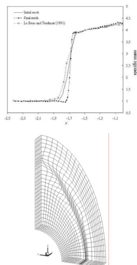
The specific mass distribution along the stagnation line and final mesh are presented in Fig. 4, where it is observed the difference between the gradients obtained with the initial and final mesh. The distribution exhibits smooth behavior without instability in the stagnation region. The specific mass distribution on the stagnation line and the stand-off distance of the shock are in good agreement with numerical results obtained by Le Beau and Tezduyar (1991).
Figure 3. Geometric and boundary conditions to simulate the flow around a circular cylinder.
Figure 4. Specific mass distribution on the stagnation line and final mesh over a circular cylinder.
The final mesh is obtained after 4 adaptations. It can be observed that elements and nodes are concentrated in the region where strong shock wave exists. Note that elements located near the surface AB preserve their edges in the circumferential and radial directions because the mesh topology in this zone follows approximately the bow shock. On the other hand, near the outflow region (surface CD) elements are distorted, taking the appearance of rhombus because the bow shock switches from the circular curves family to the radial curves family along a transition region.
Supersonic Flow over a Bump
In this example, the current methodology is applied to a steady supersonic flow over a bump arc that is well documented in the paper of Le Beau et al. (1993). The bump arc is placed on the floor of a frictionless wind tunnel and it is describe by:
(
)
(
2)
0 . 0 4 1 4 1 . 5
y= − x− with 1≤ ≤x 2 (20)
The bump lies in the center of the bottom boundary of the domain, which is extended 1 unit in front and behind the bump, and 1 unit above. The freestream has a Mach number equal to 1.4 and a dimensionless specific mass equal to 1.0. An oblique shock forms at the leading edge, as expected, and it is reflected at the upper-symmetry boundary. This case was computed using a mesh with
pressure contours in the neighborhood of the bump for the initial mesh and the final mesh is shown in Fig. 6. The final mesh require 6 levels of adaptation respectively and it may be observed that the elements are aligned with the shock wave maintaining a high quality mesh.
The specific mass distribution along the center of the channel is shown in Fig. 7. It can be observed that the solution obtained with the initial mesh is close to the results obtained by Hendriana and Bathe (2000) with reference to the position of the shock wave as well as its intensity. Results obtained by Le Beau et al. (1993) are not shown in Fig. 7, but they are similar to those obtained in the present work, excepting in the trailing edge region, where some small differences were observed. With the adaptation procedure proposed in this work, a decrease in the shock thickness and an increase in its intensity were obtained with respect to the results presented using the initial mesh and with respect to those given by the aforementioned references, while the position of the shock wave was preserved. Le Beau et al. (1993) used a fine mesh with
184 x 60 bi-linear quadrilateral elements and Hendriana and Bathe
(2000) used a mesh with 15 x 46 parabolic quadrilateral elements.
Figure 5. Final adaptive mesh over a bump.
Figure 6. Initial and final distribution of pressure over a bump.
Figure 7. Distribution of specific mass along the center of the channel.
Supersonic Flow around a Sphere
A steady supersonic flow past a sphere with a dimensionless value of the radius equal to 1 is considered in this example. Only a quarter part of the sphere is taken into account because of geometrical symmetry. The freestream flow has a Mach number
3.0
M∞= . The boundary conditions are the same employed in the
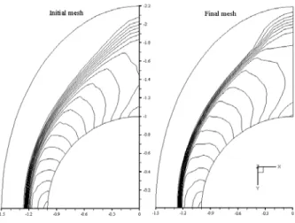
case of the circular cylinder. The domain is discretized using a mesh with 8424 elements containing 9625 nodes. In Fig. 8 the initial and final meshes are shown. Only the part of the final mesh corresponding to the plane x - y is depicted in this figure. Note that near the outflow region, the mesh has the same behavior as the case of the circular cylinder.
Figure 8. Initial mesh and final mesh contained in the plane x-y.
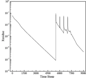
A plot of the convergence history for the solution using 4 times the mesh adaptation procedure is presented in Fig. 9. This figure presents the variation of the residue of the specific mass verified in the flow field. The jumps in the curve occurs when the mesh is adapted, as a consequence of the re-evaluation of the solution of the old mesh, this re-evaluated solution is used in the new adapted mesh.
Figure 9. Convergence history for the supersonic flow around a sphere.
Figure 10. Comparison of the Mach number for both meshes.
An analytical expression to obtain the value of the pressure at
the stagnation point
( )
ps is given in the Report 1135 (1953) of theNational Advisory Committee for Aeronautics (Ames Research Staff). With this expression the corresponding values is
12,06
s
p p∞= , while ps p∞=12,33 was obtained with the
present numerical simulation.
The pressure and Mach number distributions in the stagnation line are presented in Fig. 11. It is clear that the shock computed on the adapted mesh is better than those obtained with the initial mesh. One also notes the absence of oscillations before and after the
shock. The stand-off distance D may be calculated analytically by
the expression given by Ambrosio and Wortman (1962), which is referenced in Argyris et al. (1990). The corresponding value is
0.210
D= , while D=0.234 was obtained with the present
numerical simulation.
Figure 11. Pressure distribution in the stagnation line.
Conclusions
The development of a simple and computationally effective methodology to adapt finite element meshes to simulate compressible flows with strong shock waves was the main objective of this work. The nodal re-allocation adaptivity, used in this study, starts from an initial mesh and the grids are concentrated in the desired region without any grid tangling. The method is characterized by the error estimation measured in the element edges using a Riemann metric, which is defined employing the Hessian matrix. An optimization procedure is used to preserve as well as possible mesh orthogonality, smoothness and equidistribution of the
error. Good results for supersonic flows were found, showing that they were improved using the adaptive procedure with respect to those obtained with the initial mesh. It is important to highlight that meshes with good quality were attained for the four cases studied here.
The effectiveness of this method to improve the solution is limited by the number of nodes in the initial mesh. Nevertheless,
this r-method should ideally complement the h-method. Moving
mesh methods are better to reduce dispersive errors in the vicinity of high gradients, while local refinement methods can, in principle, add enough nodes to solve any fine scale structure. We expect that combining mesh movement with local refinement generally will not
only make the global error control possible for the r-method, but
also avoid the need of excessive local refinements, and produce mesh that are better aligned with and closely follow the solution features.
Acknowledgments
The development of this work has been supported by the agency CAPES by means of a master´s fellowship.
References
Ait-Ali-Yahia, D., 1996, “A Finite Element Segregated Method for Thermo-Chemical Equilibrium and Nonequilibrium Hypersonic Flows using Adated Grids”, Ph.D. Thesis, Deparment of Mechanical Engineering, Concordia University, Canada, 167 p.
Ait-Ali-Yahia, D., Habashi, W.G. and Tam, A., 1996, “A Directionally Adaptive Methodology Using an Edge-Based Error Estimate on
Quadrilateral Grids”, International Journal for Numerical Methods in
Fluids, Vol. 23, pp. 673-690.
Ait-Ali-Yahia, D. and Habashi, W.G., 1997, “Finite Element Adaptive
Method for Hypersonic Thermochemical Nonequilibrium Flows”, AIAA
Journal, Vol. 35, pp. 1294-1302.
Ames Research Staff, 1953, “Report 1135: Equations, Tables, and
Charts for Compressible Flow”, National Advisory Committee for
Aeronautics.
Argyris, J., Doltsinis, I.S. and Friz, H., 1990, “Studies on Computational
Reentry Aerodynamics”, Computer Methods in Applied Mechanics and
Engineering, Vol. 81, pp. 257-289.
Bono, G., 2004, “Adaptação via Movimento de Malhas em Escoamentos Compressíveis” (in Portuguese), M.Sc. Thesis, PROMEC, Universidade Federal do Rio Grande do Sul, Brazil, 126 p.
Bono, G., 2008, “Simulação Numérica de Escoamentos em Diferentes Regimes utilizando o Método dos Elementos Finitos” (in Portuguese), Doctoral Thesis, PROMEC, Universidade Federal do Rio Grande do Sul, Brazil, 183 p.
Brackbill, J.U. and Saltzman, J.S., 1982, “Adaptive Zoning for Singular
Problems in Two Dimensions”, Journal of Computational Physics, Vol. 44,
pp. 342-368.
Cao, W., Huang, W. and Russell, R.D., 1999, “An r-Adaptive Finite
Element Method Based Upon Moving Mesh PDEs”, Journal of
Computational Physics, Vol. 149, pp. 221-244.
Carcaillet, R., Dulikravich, G.S. and Kennon, S.R., 1986, “Generation of
Solution-Adaptive Computational Grids Using Optimization”, Computer
Methods in Applied Mechanics and Engineering, Vol. 57, pp. 279-295. Christon, M.A., 1997, “A Domain-Decomposition Message-Passing Approach to Transient Viscous Incompressible Flow Using Explicit Time
Integration”, Computer Methods in Applied Mechanics and Engineering,
Vol. 148, pp. 329-352.
Donea, J., 1984, “A Taylor-Galerkin Method for Convective Transport
Problems”, International Journal for Numerical Methods in Engineering,
Vol. 20, pp. 101-119.
Gnoffo, P.A., 1983, “A Finite-Volume , Adaptive Grid Algorithm
Applied to Planetay Entry Flow Fields”, AIAA Journal, Vol. 21, No. 9, pp.
1249-1254.
Hawken, D.F., Gottlieb, J.J. and Hansen, J.S., 1991, “Review of Some Adaptive Node-Movement Techniques in Element and
Finite-Difference Solutions of Partial Differential Equations”, Journal of
Hendriana, D. and Bathe, K.J., 2000, “On a Parabolic Quadrilateral
Finite Element for Compressible Flows”, Computer Methods in Applied
Mechanics and Engineering, Vol. 186, pp. 1-22.
Kennon, S.R. and Dulikravich, G.S., 1986, “Generation of
Computational Grids Using Optimization”, AIAA Journal, Vol. 24, pp.
1069-1073.
Kessler, M.P. and Awruch, M.A., 2004, “Analysis of Hipersonic Flows
Using Finite Elements with Taylor-Galerkin Scheme”, International Journal
for Numerical Methods in Fluids, Vol. 44, pp. 1355-1376.
Le Beau, G.J., Ray, S.E., Alibadi S.K. and Tezduyar, T.E., 1993, “SUPG Finite Element Computation of Compressible Flows with the
Entropy and Conservation Variables Formulations”, Computer Methods in
Applied Mechanics and Engineering, Vol. 104, pp. 397-422.
Le Beau, G.J. and Tezduyar, T.E., 1991, “Finite Element Computation of Compressible Flows with the SUPG Formulation”, FED-Advances in Finite Element Analysis in Fluid Dynamics, ASME, Vol. 123, pp. 21-27.
Löhner, R., 2001, “Applied CFD Techniques. An Introduction based on
Finite Element Methods”, John Wiley & Sons Ltd., England, 366 p.
Nakahashi, K. and Deiwert, G.S., 1987, “Self-Adaptive Grid Method
with Application to Airfoil Flow”, AIAA Journal, Vol. 25, No. 4, pp.
513-520.
Peraire, J., Vahdati, M., Morgan, K. and Zienkiewicz, O.C., 1987,
“Adaptive Remeshing for Compressible Flow Computations”, Journal of
Computational Physics, Vol. 72, pp. 449-466.
Press, W.H., Teukolsky, S.A., Vetterling, W.T. and Flannery, B.P., 1992, “Numerical Recipes in Fortran 77”, Cambridge University Press, England, pp. 413-417.
Tam, A., Ait-Ali-Yahia, D., Robichaud, M.P., Moore, M., Kozel, V., Habashi, W.G., 2000, “Anisotropic Mesh Adaptation for 3D Flows on
Structured and Unstructured Grids”, Computer Methods in Applied