Intercomparison and assessment of turbulent and physiological exchange parameters of grassland

(1)

BGD

6, 241–290, 2009

Turbulent and physiological exchange parameters

of grassland

E. Nemitz et al.

Title Page

Abstract Introduction

Conclusions References

Tables Figures

◭ ◮

Back Close

Full Screen / Esc

Printer-friendly Version

Interactive Discussion Biogeosciences Discuss., 6, 241–290, 2009

www.biogeosciences-discuss.net/6/241/2009/ © Author(s) 2009. This work is distributed under the Creative Commons Attribution 3.0 License.

Biogeosciences Discussions

Biogeosciences Discussionsis the access reviewed discussion forum ofBiogeosciences

Intercomparison and assessment of

turbulent and physiological exchange

parameters of grassland

E. Nemitz1, K. J. Hargreaves1, A. Neftel2,*, B. Loubet3, P. Cellier3, J. R. Dorsey4,**, M. Flynn4,**, A. Hensen5, T. Weidinger6, R. Meszaros6, L. Horvath7,

U. D ämmgen8, C. Fr ühauf8, F. J. L öpmeier9, M. W. Gallagher4, and M. A. Sutton1

1

Atmospheric Sciences, Centre for Ecology and Hydrology (CEH) Edinburgh, Bush Estate, Penicuik, Midlothian, EH26 0QB, UK

2

Agroscope Reckenholz-T ¨anikon Research Station ART, 8046 Z ¨urich, Switzerland

3

Institut National de la Recherche Agronomique (INRA), UMR Environnement et Grandes Cultures, Thiverval-Grignon, 78850, France

4

School of Earth, Atmospheric and Environmental Sciences, University of Manchester, Simon Building, Oxford Road, Manchester, M13 9PL, UK

5

Energy research Centre of the Netherlands (ECN), Postbus 1, 1755 ZG Petten, The Netherlands

6

E ötv ös Lor ánd University, Department of Meteorology, 1117 Budapest, Hungary

7

(2)

BGD

6, 241–290, 2009

of grassland

E. Nemitz et al.

Title Page

Tables Figures

◭ ◮

Back Close

Full Screen / Esc

Interactive Discussion

8

Institute for Agroecology, German Agricultural Research Institute, Braunschweig-V ¨olkerode, Germany

9

Agrometeorological Research Station of Deutscher Wetterdienst, Bundesallee 50, 38116 Braunschweig, Germany

*formerly known as the Swiss Federal Research Station for Agroecology and Agriculture (FAL-IUL)

**formerly known as the University of Manchester Institute of Science and Technology (UMIST)

Received: 22 September 2008 – Accepted: 11 October 2008 – Published: 8 January 2009

Correspondence to: E. Nemitz (en@ceh.ac.uk)

(3)

BGD

6, 241–290, 2009

of grassland

E. Nemitz et al.

Title Page

Tables Figures

◭ ◮

Back Close

Full Screen / Esc

Abstract

Commonly, the micrometeorological parameters that underline the calculations of sur-face atmosphere exchange fluxes (e.g. friction velocity and sensible heat flux) and pa-rameters used to model exchange fluxes with SVAT-type parameterisations (e.g. latent heat flux and canopy temperature) are measured with a single set of instrumentation

5

and are analysed with a single methodology. This paper evaluates uncertainties in these measurements with a single instrument, by comparing the independent results from nine different institutes during the international GRAMINAE integrated field exper-iment over agricultural grassland near Braunschweig, Lower Saxony, Germany. The paper discusses uncertainties in measuring friction velocity, sensible and latent heat

10

fluxes, canopy temperature and investigates the energy balance closure at this site. Although individual 15-min flux calculations show a large variability between the instru-ments, when averaged over the campaign, fluxes agree within 2% for momentum and 11% for sensible heat. However, the spread in estimates of latent heat flux (λE) is larger, with standard deviations of averages of 18%. While the dataset averaged over

15

the different instruments fails to close the energy budget by 30%, if the largest turbulent fluxes are considered, near perfect energy closure can be achieved, suggesting that most techniques underestimateλE in particular. The uncertainty inλE feeds results in an uncertainty in the bulk stomatal resistance, which further adds to the uncertainties in the estimation of the canopy temperature that controls the exchange. The paper

20

demonstrated how a consensus dataset was derived, which is used by the individual investigators to calculate fluxes and drive their models.

1 Introduction

When measuring surface/atmosphere exchange fluxes of trace constituents at the canopy scale, usually one single set of instrumentation is used to provide the

microme-25

(4)

BGD

6, 241–290, 2009

of grassland

E. Nemitz et al.

Title Page

Tables Figures

◭ ◮

Back Close

Full Screen / Esc

Interactive Discussion is true for the measurement of parameters that are used to drive parameterisations

and models to predict the exchange, usually in the form of soil-vegetation-atmosphere transport (SVAT) models. Key parameters are wind speed (u), friction velocity (u∗) and the sensible heat flux (H) for the calculation of fluxes, while the parameterisations require input of photosynthetically active radiation (PAR) or solar radiation (St), air tem-5

perature (T_a), canopy temperature (T_c) and relative humidity (RH).

This paper utilises measurements made during the GRAMINAE Integrated Experi-ment at Braunschweig, Germany, to investigate the effect of differences between ap-proaches and uncertainties in the results, using an array of instrumentation operated and analysed by a number of independent institutes. The main aim of the

experi-10

ment was to investigate the dynamics of ammonia exchange between grassland and the atmosphere, as described in detail in accompanying papers (Sutton et al., 2008a). The flux analysis techniques were deliberately not standardised, although all groups involved have extensive experience in the application of eddy-covariance techniques. Pure instrument comparisons have been presented elsewhere (e.g. Dyer et al., 1982;

15

Tsvang et al., 1985; Fritschen et al., 1992; Christen et al., 2000). Instead, this paper focuses on the differences that may be expected to be introduced by a combination of differences in instrumentation, chosen measurement height and analysis protocols, as they would be applied by individual groups in real applications.

The measurements included fluxes of momentum and sensible heat made with a

to-20

tal of 10 independent ultrasonic anemometers, operated by 9 different institutes from 5 different countries and analysed according to their respective protocols. Variability in the results is discussed, together with the strengths and weaknesses of the different techniques and, as a quality control, the closure of the energy budget is explored. The paper also compares different ways to establish the leaf temperature that controls

bio-25

genic emissions and investigates the propagation of errors into the paramaterisation of bulk stomatal resistance at this site.

(5)

BGD

6, 241–290, 2009

of grassland

E. Nemitz et al.

Title Page

Tables Figures

◭ ◮

Back Close

Full Screen / Esc

Interactive Discussion analyses (Meszaros et al., 2008; Sutton et al., 2008b; Burkhardt et al., 2008; Loubet

et al., 2009; Milford et al., 2008; Meszaros et al., 2008; Sutton et al., 2008b; Personne et al., 2008). At the same time, the intercomparison of the paper provides the basis to assess uncertainties in the measurement of turbulent exchange parameters, which is particularly relevant to the more usual interpretation of measured fluxes where only

5

one set of sensors is available.

2 Theory

2.1 Eddy-covariance approach for measuring turbulent exchange fluxes

Several micrometeorological approaches are available to measure fluxes of momentum and heat at the canopy scale. The two approaches used here are the aerodynamic

gra-10

dient method (AGM) and the eddy-covariance (EC) technique, which have extensively been described in the literature (Sutton et al., 1993).

Eddy-covariance measures the flux (Fχ) of a scalarχ directly as the covariance

F_χ =w′_χ′₌_wχ₋_{w χ} ₍₁₎

wherew′andχ′are the instantaneous deviations about the mean, of the vertical wind

15

velocity (m s−1) and the scalar, respectively. For measurements above homogeneous flat terrain, w is expected to be zero and a non-zero value is usually attributed to a misalignment of the wind sensor. Therefore, a co-ordinate rotation is performed by all groups taking part in the Braunschweig experiment, to alignuwith the mean wind.

For this study, momentum flux (τ), sensible heat flux (H) and latent heat flux, λE 20

(W m−2) were derived directly from the eddy covariance measurements using equa-tions equivalent to Eq. (1):

τ=ρw′_u′ ₍₂₎

(6)

BGD

6, 241–290, 2009

of grassland

E. Nemitz et al.

Title Page

Tables Figures

◭ ◮

Back Close

Full Screen / Esc

λE = λρε

P w′e′ (4)

whereρis the density of air (kg m−3),cpis the heat capacity of air (J g−

1

K−1),λis the latent heat of evaporation of water (J kg−1), εis the ratio of the molecular weights of water and air (=0.622) andP is atmospheric pressure (kPa).

The friction velocity (u∗) may be calculated from the turbulence measurements as:

5

u∗=

r

−τ

ρ = q

−u′_w′ ₍₅₎

or

u∗= 4

q

(u′_w′₎2₊₍_v′_w′₎2_, ₍₆₎

both of which are used by different institutes. In atmospheric turbulence, the covariance between the stream-wise wind component (u) and the horizontal cross-wind

compo-10

nent (v) is expected to be small. In addition to the previously described co-ordinate rotation around two axes, a third rotation was used here by individual groups to set this covariance to zero (Aubinet et al., 2000).

2.2 The aerodynamic gradient approach for measuring turbulent exchange fluxes

Eddy-covariance approaches can only applied for compounds for which fast-response

15

sensors are available for measurement at a frequency for several Hz. For many highly reactive compounds such sensors do not generally exist, and here alternative, parame-terised techniques are applied, which can utilise slow response measurements. Fluxes may be calculated as

Fχ =−u∗ χ∗ (7)

(7)

BGD

6, 241–290, 2009

of grassland

E. Nemitz et al.

Title Page

Tables Figures

◭ ◮

Back Close

Full Screen / Esc

Interactive Discussion whereu∗and χ∗ may be derived from time-averaged gradient measurements, using

the aerodynamic flux-gradient relationships (e.g. Flechard and Fowler, 1998):

u∗=−k d u

d[ln(z−d)−ΨM z−_Ld]

(8)

and

χ∗=−k d χ

d[ln(z−d)−ΨH z−_Ld]

. (9)

5

Note that in the literature the aerodynamic gradient approach is more often introduced in terms of a local gradient (d χ /d z) of the logarithmic profile, or the differences be-tween two heights ((χ2−χ1)/(z2−z1)). However, we present the approach in the (math-ematically identical) form of a linear gradient (Eq. 8), as this can more easily be derived from measurements at more than 2 heights, by linear regression. In Eqs. (8) and (9),

10

k is von Karman’s constant (0.41) and χ is the mean scalar concentration at height (z−d),z is the height above the ground,d is the zero-plane displacement height, and ΨM and ΨH are the dimensionless integrated stability correction terms for momen-tum and heat, which can be calculated from the height and atmospheric stability as parameterised through the Monin-Obukhov length (L):

15

L=−u∗

3

ρ c_pT

kgH , (10)

wheregis the acceleration due to gravity (m s−2). Various formulations for calculating these stability corrections have been presented in the literature. In practice, a hybrid approach is often used, whereu∗in Eq. (7) is derived by ultrasonic anemometry, while

χ∗is derived from averaged concentration profiles according Eq. (9).

(8)

BGD

6, 241–290, 2009

of grassland

E. Nemitz et al.

Title Page

Tables Figures

◭ ◮

Back Close

Full Screen / Esc

Interactive Discussion 2.3 Resistance analogy

For the purposes of determining the processes controlling the exchange of scalars such as ammonia, ozone, sulphur dioxide and nitrogen oxides, it is necessary to calculate the resistances to turbulent exchange. In the case of consistently deposited species it is often assumed that the concentration of the scalar at the absorbing surface is zero

5

such that

R_t(z−d)=R_a(z−d)+R_b+R_c (11)

whereRt is the total resistance to transfer, Ra is the aerodynamic resistance, Rb is the laminar boundary-layer resistance close to the surface of the leaves andR_c is the canopy resistance. The aerodynamic resistance, R_a, at (z−d)=1 m is obtained from

10

Garland (1977):

R_a(1)= u(1)

u∗2 −

ψ_h 1

L

−ψ_m 1

L

ku∗ (12)

where the second r.h.s. term is zero in neutral and stable conditions. For the calculation ofR_b, Owen and Thompson (1963) used the relationship

R_b=(Bu∗)−1 (13)

15

whereB, the sub-layer Stanton number was defined by Garland (1977) as

B−1=1.45Re_∗0.24Sc0.8. (14)

Here, the roughness Reynold’s number,Re_∗, is given by

Re_∗= z0_νu∗ (15)

and the Schmidt number, Sc, by

20

Sc= ν

(9)

BGD

6, 241–290, 2009

of grassland

E. Nemitz et al.

Title Page

Tables Figures

◭ ◮

Back Close

Full Screen / Esc

Interactive Discussion whereν is the kinematic viscosity of air (m2s−1), D is the diffusion coefficient of the

scalar of interest (m2s−1). There are a number of alternative approaches to calculate the sub-layer Stanton number (Wesely and Hicks, 1977; Sutton et al., 1993), but in practice the differences forR_bare small for short vegetation. It should be noted thatR_b

is specific for each chemical species, due to differences inD.

5

For chemical species that are exchanged with the plant through the leaf stomata, but not with the soil or leaf cuticles,R_c may be substituted by the bulk stomatal resis-tance (R_sb). In other cases, where stomatal exchange is only one of several exchange pathways,Rc may often be represented by a resistance network which contains Rsb (Shuttleworth and Wallace, 1985; Sutton et al., 1998; Nemitz et al., 2001). For water

10

vapour, if it is assumed that over a transpiring canopy with dry leaf surfaces, the bulk of the latent heat flux is transported via the stomates, then it is possible to calculate a bulk stomatal resistance,R_sb, from vapour pressure at the leaf surface,e(z′₀) and saturated vapour pressure at the leaf surface temperature,e_s(T(z₀′)) as:

R_sb= es(T(z ′

0))−e(z ′ 0)

E (17)

15

The surface values can be calculated for a notional mean height of the canopy ex-change (z′₀), from the values at a reference height (zref) and the turbulent fluxes, as-suming the canopy to act as a big leaf:

T(z′₀)=T(zref)+

H ρcp

(Ra(zref)+Rb,H) (18)

and

20

(10)

BGD

6, 241–290, 2009

of grassland

E. Nemitz et al.

Title Page

Tables Figures

◭ ◮

Back Close

Full Screen / Esc

3 Methods

3.1 Field site

A full description of the field site, measurement periods and site management may be found elsewhere (Sutton et al., 2008a). The field site was aLolium periennedominated agricultural grassland, which was cut 10 days into the 27 day measurement period (19

5

May to 15 June 2000), from 0.7 to 0.07 m canopy height, and which grew to 0.35 m by the end of the campaign. A large array of micrometeorological equipment was de-ployed over the canopy by several groups from different European research institutes. The bulk of this equipment was placed at “Site 1” (Loubet et al., 2009); in practice the sensors were distributed along a roughly north-south axis covered a distance of about

10

100 m along a transect through the field. The available fetch was approximately 300 m to the west and east of Site 1, 200 m to the south and 50 to 100 m to the north. A fur-ther, smaller array of instruments was located at “Site 2”, approximately 250 m east of Site 1 and close to the eastern edge of the field, which was bounded to the east by a deciduous shelterbelt approximately 8 m tall. The participating research groups and

15

the abbreviations used for each have been presented elsewhere (Hensen et al., 2008).

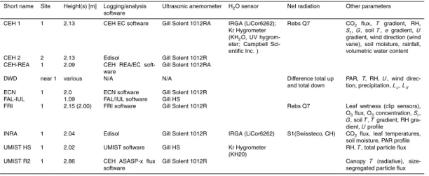
3.2 Instrumentation deployment

The measurements analysed here were made at nine eddy flux towers, all of which were equipped with an ultrasonic anemometer to measure fluxes of momentum and sensible heat. Only one of these eddy towers was operated at Site 2, while four towers

20

also measured fluxes of latent heat (Table 1).

In addition to the eddy covariance measurements reported here, momentum fluxes and sensible heat fluxes were also derived from 2 wind-speed gradients (using cup anemometers) and 3 temperature profiles (using fine theromocouples). As these mea-surements showed larger variability than the eddy-covariance meamea-surements, it was

25

(11)

BGD

6, 241–290, 2009

of grassland

E. Nemitz et al.

Title Page

Tables Figures

◭ ◮

Back Close

Full Screen / Esc

Interactive Discussion with the dewpoint hygrometer profile of a Bowen ratio system (Campbell Scientific).

These measurements were rejected as the response time of the hygrometer was found to be insufficient for the switching frequency between the two heights, despite having followed the manufacturer’s guidelines. Several setups, including the nearby station of the German Weather Service (DWD), included measurements of solar radiation (St), 5

photosynthetically active radiation (PAR) or net radiation (R_n), as well as absolute tem-perature and relative humidity. Here, the measurements ofR_n are compared to inves-tigate the effect of uncertainties inRnon the energy budget closure. It should be noted that most groups also deployed a range of chemical analysers for gases and aerosols at each location, but these are described in the accompanying papers within this issue

10

(Hensen et al., 2008b; Meszaros et al., 2008; Milford et al., 2008; Nemitz et al., 2008). Several of the sonic anemometers formed part of relaxed eddy accumulation (REA) systems for NH3(CEH REA; ECN and FAL-IUL) (Hensen et al., 2008b).

All groups calculated averaged data every 15 min, and clocks were synchronised to UTC (GMT) (local time minus two hours). The comparatively short averaging period

15

was chosen because it was felt that the high time-resolution would maximize the in-formation on NH₃ exchange processes. The frequency at which the spectral density functions peak increases linearly with measurement height. It was therefore estimated that the 15 min calculations at a height of about 2 m over the smooth grassland veg-etation is at least comparable to an averaging time of 30 min over forest (Kaimal and

20

Finnigan, 1994). The validity of this estimate is discussed below.

Slow sensors such as the different components of the gradient systems were recorded on data loggers (Model 21X, Campbell Scientific), while all fast data were recorded on PCs. With the exception of INRA and CEH 2, who used the commercial logging and analysis software Edisol 2.0 (Moncrieffet al., 1997), all institutes applied

25

(12)

BGD

6, 241–290, 2009

of grassland

E. Nemitz et al.

Title Page

Tables Figures

◭ ◮

Back Close

Full Screen / Esc

Interactive Discussion 3.3 Data analysis

The first stage of data analysis was performed by the individual research groups and involved filtering of the 15-min flux data to remove periods of instrument calibration, instrument malfunction or power failure. This coarsely filtered data was then drawn together and subjected to the following filtering procedure: the exact position of each

5

instrument mast in relation to the other masts, mobile laboratories and other obstruc-tions to the fetch was determined and all flux data falling within obstructed sectors were removed from that individual dataset. Where more than one group measured an individual parameter, the median of each of wind direction (dd), u∗,H, and λE from the eddy covariance systems, together withSt, Rn and PAR were then calculated and 10

carried forward in the analysis to allow the validity of each individual dataset to be assessed by comparison with the median data.

In the case ofdd this was performed by a simple inspection of the time-series plots to confirm that no gross alignment errors were evident. The assessment of the extent to which each individual dataset was representative of the “consensus” dataset (cf.

15

Sect. 4.10), consisted of performing a least-squares linear regression of the individual dataset on the median dataset.

In addition, values of the estimated length of fetch available for the wind direction observed during each 15 min period, and the cumulative normalised footprint (CNF after Kormann and Meixner, 2001) function were calculated and included in the

con-20

sensus dataset. Flags were also provided for each 15 min value to indicate whether the measurements were in any way compromised by field conditions, thus allowing individual groups to filter the data according to their specific needs. Specifically, un-suitable micrometeorological conditions were defined as occurring under any of the following conditions: u (1 m) <0.8 m s−1; −5 m<L<+5 m; CNF<67% within the fetch.

25

(13)

BGD

6, 241–290, 2009

of grassland

E. Nemitz et al.

Title Page

Tables Figures

◭ ◮

Back Close

Full Screen / Esc

Interactive Discussion al. (2002), by definingI(T) such that:

I(T)= 1

τ T Z

0

w′χ′d t; 0≤T ≤τ. (20)

The value ofI(T) was regressed on T for each 15 min averaging period and the stan-dard deviation of the regression line (σf), used to calculate the relative stationarity coefficient (ζ) as

5

ζ= 2σf

w′_χ′ (21)

and periods of instationarity were defined asζ >1.2.

A consensus time-series of the zero plane displacement height (d) was derived from comparison of eddy-covariance results with the profile measured with cup anemome-ters (Vector Instruments) at 6 heights. For periods of near neutral stability (ΨM≈0) 10

the value of d in Eq. (8) was adjusted until the gradient estimate of u∗ matched the consensus value. This exercise was repeated for periods of varying h_c, to develop a relationship betweend and hc, which was then used to derived a continuous time series ofd (shown in Fig. 8a).

4 Results

15

4.1 Initial data reduction

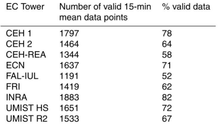
The first and second stages of data analysis (data filtering by institutes and filtering in relation to bad wind sectors) resulted in a reduction of the quantity of suitable flux data to between 52 and 82% at the individual measurement sites (Table 2). This reduction in data was a reflection principally of the degree of obstruction the individual masts

20

(14)

BGD

6, 241–290, 2009

of grassland

E. Nemitz et al.

Title Page

Tables Figures

◭ ◮

Back Close

Full Screen / Esc

Interactive Discussion In the following sections the different estimates are compared against a consensus

dataset derived for Site 1. This was calculated as the average of those instruments that were deemed to provide equally reliable measurements for this site, as described in more detail below (Sect. 4.10).

4.2 Comparison of momentum fluxes

5

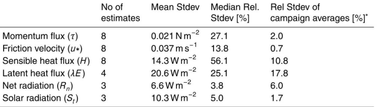
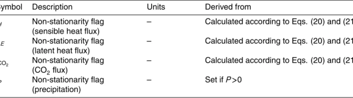
The comparison of the analysis of surface stress, or momentum flux (τ) is presented in Fig. 1a to g. This indicates that with the exception of ECN (Fig. 1c), the average values ofτfor each individual mast at Site 1 lie within+7.9% and−7.7% of the median value (as derived as the deviation of the slope from unity) an agreement judged to be very encouraging in view of the relatively large spatial distribution of masts in the field

10

and the diverse nature of the anemometry, measurement height and eddy covariance software employed. While the median standard deviation between measurements for each 15 min period lies at 27.1%, averaged over the campaign, the standard deviation decreases to 2.0% (Table 3). This indicates that differences are due to spatial and temporal fluctuations in the turbulence, rather than systematic differences.

15

Although the ECN data showed a discrepancy of−16.1% compared to the median, inspection of Fig. 1c shows that the least-squares regression was skewed by a rela-tively small number of scattered data points at low u∗ values and that the bulk of the data points lie along the 1:1 line. It was therefore decided to retain the ECN data within the consensus dataset for τ and u∗. The ECN data were taken as part of the ECN

20

REA system and its data acquisition was not optimized for eddy-covariance applica-tion. Thus, although the system calculated the parameters needed for the REA cal-culations online, over suitable averaging periods, eddy-covariance results were stored every minute and had to be averaged in post-processing to provide 15-min values. Here additional assumptions had to be made to estimate the contribution of eddies in

25

the frequency range between 1 and 15 min, explaining the higher variability.

(15)

BGD

6, 241–290, 2009

of grassland

E. Nemitz et al.

Title Page

Tables Figures

◭ ◮

Back Close

Full Screen / Esc

Interactive Discussion consensus calculation on the basis that the spatial separation was in excess of 100 m

and the mast was relatively close to the shelter belt at the eastern end of the field, although easterly winds were removed from the CEH EC2 dataset, when filtering for obstructed wind sectors.

Whileτ is the fundamental parameter, the parameter needed for the flux calculation

5

is actually the friction velocity, for which the equivalent correlation plots are shown in Fig. 2. Due to the close link between u∗and τ, the scatter plots for u∗ show similar features.

4.3 Comparison of sensible heat flux

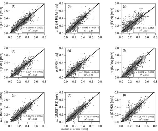
All sensible heat fluxes were calculated using the individual ultrasonic anemometers

10

calculation of temperature based on the speed of sound in air. The results of the regression analysis are presented in Figs. 3a to h for Site 1, and in Fig. 3i for the single instrument at Site 2. For the majority of the instruments the discrepancy in the slope of the regression against the median value of H lay in the range +5.3 and −6.9%, while the intercept, was less than 2 W m−2, indicating how consistently the transition

15

from unstable to stable conditions was measured. The exception to this rule was the ECN results, which again showed considerable scatter, for the reason described in the previous section. No systematic differences were found between different anemometer types.

4.4 Latent heat flux

20

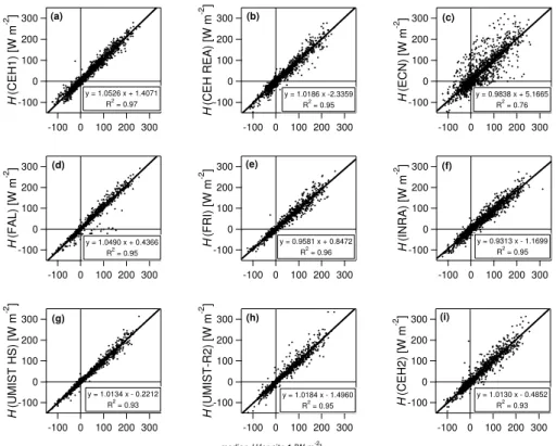
Latent heat fluxes were measured solely at Site 1 using two open-path sensors of CEH and UMIST (Fig. 4a and d) and two closed-path sensors of INRA and CEH (Fig. 4b and c). Details of the different instruments used are summarized in Table 1.

Agreement between the four instruments for latent heat flux was poorer than that for sensible heat or momentum flux, with the CEH open- and closed-path instruments

25

(16)

BGD

6, 241–290, 2009

of grassland

E. Nemitz et al.

Title Page

Tables Figures

◭ ◮

Back Close

Full Screen / Esc

Interactive Discussion UMIST system an upper bound. Possible reasons are discussed below (Sect. 5.2).

4.5 Net radiation

During the GRAMINAE integrated experiment at Braunschweig, fluxes of ammonia and other trace gases were either calculated by eddy-covariance (fluxes of latent and sensi-ble heat, momentum, ozone, particles), hybrid aerodynamic gradient techniques (with

5

theu∗ taken from sonic anemometery, NH3, acid gases) or relaxed eddy accumula-tion (NH3). Hence, net radiation (Rn) was not needed for the flux calculations per se as it would be the case in Bowen ratio or modified Bowen ratio techniques. However, the accuracy with whichRn can be measured is important for the interpretation of the energy balance closure at this site. In addition, R_n was needed to drive some of the

10

numerical models, which incorporated their own heat balance calculation (Personne et al., 2008).

Three of the four net radiometers were operated at Site 1, while the fourth was operated at the DWD compound, 200 m to the SW, over continuously short “standard” grassland. The net radiometers were typically mounted at a height of 2 m and their

foot-15

print is therefore very different to that of the turbulent flux measurements. The CEH and FRI radiometers in particular showed a very tight relationship, while the INRA instru-ment shows some more variability. The DWD radiometers reported significantly smaller values ofR_n (Fig. 5b). These were calculated as the difference of a measurement of total downward radiation and total upward radiation. Substitution of the measurement

20

of total downward radiation by the sum of an alternative estimate of shortwave down-ward radiation (S_t) and long-wave downward radiation (both also from DWD) provided much better agreement (R_n (DWD, alternative)=1.019×R_n(consensus)+18.2 W m−2;

R2=0.963, not shown). However, since these alternative values were only reported at hourly resolution (rather than 15 min resolution) and since the management of the

25

(17)

BGD

6, 241–290, 2009

of grassland

E. Nemitz et al.

Title Page

Tables Figures

◭ ◮

Back Close

Full Screen / Esc

Interactive Discussion 4.6 Ground heat flux

Ground heat fluxes at the soil surface (G) were derived with two semi-independent sys-tems as part of the setups of CEH and FRI at Site 1. In both cases, soil heat fluxes were derived at a depth of 8 cm, from duplicate measurements with heat flux plates (Campbell Scientific). To this was added the heat storage in the top 8 cm, calculated

5

from changes in soil temperature (averaged over measurements at 2 and 6 cm depth within each setup, by soil thermocouples, Campbell Scientific), continuous measure-ments of the soil water content at one single site (by INRA) and measuremeasure-ments of the bulk density (average of two independent measurements of 1.35 and 1.65 g cm−3). The scatter in the comparison between the estimates ofGof the two different systems

10

(Fig. 6a) is dominated by the disagreement at times in the soil heat storage (Fig. 6c), while the soil heat fluxes agreed closely (Fig. 6b).

4.7 Closure of the energy balance

The closure in the energy balance at the site is an often used test to assess potential losses in the turbulent fluxes. In the ideal case, the net radiation (balance of up- and

15

down-ward short and long-wave components) should balance the sum of heat flux into the soil at the soil surface (G), and the turbulent fluxes of sensible heat (H) and latent heat (λE). With the consensus dataset approximately 80% energy balance closure is achieved (Fig. 7), which is typical in the range of the energy closure observed else-where (Laubach and Teichmann, 1999; Wilson et al., 2002; Oliphant et al., 2004). As

20

the array of instrumentation provides alternative answers for all parameters that feed into the assessment of the energy balance, an alternative (maximum) estimate of the energy balance closure may be compiled by considering the maximum turbulent fluxes (λE from the UMIST KH20 and H from the FAL Gill HS anemometer) and minimum

R_n(from INRA) measured during the campaign. With these extreme values almost full

25

(18)

BGD

6, 241–290, 2009

of grassland

E. Nemitz et al.

Title Page

Tables Figures

◭ ◮

Back Close

Full Screen / Esc

Interactive Discussion contributions from the increase in H (+6%) and decrease in R_n (−7%). By contrast,

choosing a single of the two ground heat fluxes (G) improves the energy balance only very little, becauseGis on average much smaller than the sum ofH andλE.

The fact that the open-path KH20 sensor of the UMIST setup derived the largestλE

may be taken as a an indication that damping effects in the sampling line and due to the

5

sensor response time are not fully compensated for in the analysis of the two closed path IRGA systems. However, theλE estimate from the CEH KH20 is also 14% lower than that of the UMIST, despite a similar sensor configuration. This may, in part, be due to the faster anemometer and improved A/D converter of the UMIST Gill HS sonic compared with the CEH Gill R2.

10

Interestingly, the largest H was derived with the FAL setup, which was operated at the lowest measurement height, where turbulence should be faster. This would be consistent with low frequency losses at an averaging time of 15 min at the higher heights (where turbulence structures are larger).

4.8 Solar radiation and PAR

15

Solar radiation (S_t) or PAR is needed to parameterise the stomatal resistance needed for SVAT modelling. The comparison of the three measurements ofS_t (by CEH, FRI and DWD) was very encouraging. CEH and FRI estimates were on average within 3% of each other, with the DWD estimate showing good agreement overall, but a larger amount of scatter. This was probably due to the spatial separation reflecting changes in

20

cloudiness at the averaging scale of 15 min. The INRA PAR sensor derived a quantum flux which was 22% higher than that measured by DWD. Hence it was decided to use the more robust estimates ofS_tfor parameterisations.

4.9 Comparison of canopy temperature estimates

Canopy temperature critically controls the potential for vegetation to react as a source

25

(19)

BGD

6, 241–290, 2009

of grassland

E. Nemitz et al.

Title Page

Tables Figures

◭ ◮

Back Close

Full Screen / Esc

Interactive Discussion linked to leaf temperature. Similarly, ammonia emission potentials (compensation

points) represent the gas phase concentration in equilibrium with the liquid phase NH+₄ concentration and the pH in the leaf apoplast. This gas-phase concentration is there-fore governed by the temperature dependence of the Henry and solubility equilibria and, at ambient temperature, approximately doubles every 5◦C (Sutton et al., 2001).

5

Thus for the correct parameterisation of the emission potential, an accurate estimate of the leaf surface temperature is paramount. We here compare three different ways of estimating leaf surface temperature:

1. A micrometeorological estimate of the average canopy temperature is calcu-lated as the surface value of the temperature, following the big-leaf approach

10

of Eq. (18).

2. An infrared radiation pyranometer (KT19.85, Heitronics GmbH, Wiesbaden) and

3. Fine thermocouple wires, mounted to the surface of leaves at different heights and senescence stages.

The intercomparison of the different measures of canopy temperature are presented

15

in Fig. 8 alongside the best estimate of the air temperature atz−d=1 m. The graph contrasts two four day example periods before and after the cut of the grassland from 0.75 m, between which the position of the thermocouples was necessarily changed.

Before the cut the vertical profile of the temperature of the green leaves is linked to light interception and the measured temperature profile in the canopy air space (not

20

shown). The pyranometer measurement closely follows the temperature of the green top leaves of the canopy. By contrast, the micromet estimate ofT(z′₀) is more closely related to the temperature of the lower leaves in the canopy (where the bulk of the biomass is located) (Herrmann et al., 2008). This estimate also shows the largest diurnal range and values which appear to be lower or higher than the temperature of

25

any physical element measured by the thermocouples.

(20)

BGD

6, 241–290, 2009

of grassland

E. Nemitz et al.

Title Page

Tables Figures

◭ ◮

Back Close

Full Screen / Esc

Interactive Discussion of the physical temperature between green leaves as well as yellow/brown and

senes-cent leaves of typically 10 K during warm days. While the pyranometer measurement reflects the temperature of the green leaves only, the micrometeorological estimate is heavily influenced by the dry vegetation.

4.10 Estimates of bulk stomatal resistance

5

The bulk stomatal resistance (Rsb) may be calculated from λE according to Eq. (17), during periods when (a)λE is dominated by evapotranspiration (leaf surfaces dry) and (b) the calculation of the surface values ofT(z′₀) ande(z′₀) is reasonably robust (R_a+R_b

small, i.e. windy conditions). Former parameterisations (Jarvis, 1976) have shown

R_sb to vary with LAI, PAR (closely related toS_t), leaf water potential and relative

hu-10

midity (or water vapour pressure deficity, VPD). Light availability is clearly the main driver for stomatal functioning. However, prolonged dry and warm periods during the Braunschweig experiment meant that drought stress also had to be taken into account, together with changes in LAI during the management of the grassland. While LAI was measured only sporadically throughout the campaign, canopy height (hc) was continu-15

ously monitored. Hence, a relationship between LAI andh_cwas derived which allowed a continuous time series of LAI to be constructed (Fig. 9a):

LAI=1.8899×ln(hc)+5.8483 (22)

where LAI is in m2m−2 and hc is in m. The measurement derived estimate ofRsb is shown as circles in Fig. 9b. It clearly responds to the cut of the grass on 29 May.

Al-20

though a parameterisation that ignores the water status (parameterised through VPD) can reproduce the measurement derived values ofRsb well on many days (Fig. 9b), it tends to under-estimate theR_sb on hot, dry days (e.g. 31 May–4 June). Inclusion of VPD into a parameterisation, based on the consensus data, leads to a much improved fit to the measurement derived values (based on Jarvis, 1976):

25

R_sb=R_sb,min

1+ b

max(0.01, St)

_LAI

ref

LAI (1−be×min(VPD,2.5)) −1

(21)

BGD

6, 241–290, 2009

of grassland

E. Nemitz et al.

Title Page

Tables Figures

◭ ◮

Back Close

Full Screen / Esc

Interactive Discussion Here R_sb is in s m−1, S_t is in W m−2 and VPD is in kPa. The fit parameters are

R_sb_,min=50 s m−1, LAIref=5.18, b=200 m2W−1 and b_e=0.31 kPa−1. As discussed in the previous section, analysis of the energy budget closure suggests that the larger UMISTλE may be a more accurate measure of the true evapotranspiration. Thus an alternative parameterisation ofR_sbwas derived to fit the UMIST data, resulting in

mod-5

ified parameters ofRsb,min=30 s m−1andbe=0.4 kPa−1. The resulting resistances are typically 40 s m−1smaller during daytime, which is similar to the contribution ofR_a+R_b

(Fig. 9c).

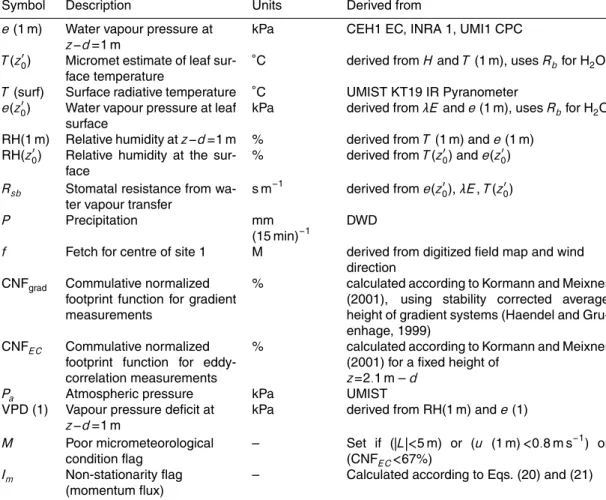
4.11 Generation of a consensus dataset

One of the reasons for the detailed intercomparison of the micrometeorological

mea-10

surements was to produce a single, consensus dataset which all participants could use for further analysis of their individual measurements, such as the calculation of gas and particle fluxes and the parameterisations of models to reproduce the exchange. The measurements summarised in the consensus dataset were based on a 15 min mean for Site 1 and are summarised in Table 4.

15

5 Discussion

5.1 Sources of discrepancy in the estimates

Comparisons between ultrasonic anemometers have been presented in the literature (Dyer et al., 1982; Tsvang et al., 1985; Fritschen et al., 1992; Christen et al., 2000; Wieser et al., 2001). In these studies an attempt was generally made to keep all

20

(22)

BGD

6, 241–290, 2009

of grassland

E. Nemitz et al.

Title Page

Tables Figures

◭ ◮

Back Close

Full Screen / Esc

Interactive Discussion Disagreement between individual sensors may generally be due to: (i) intrinsic diff

er-ences in the instrumentation and sensor response times; (ii) differences in the mounting (e.g. potential interferences from gas inlets, REA; difference in turbulence scales at dif-ferent heights); (iii) landscape heterogeneity (due to horizontal inhomogeneities and/or different footprint sizes associated with different measurement heights); (iv) statistical

5

variations and (v) differences in the analysis procedures. The relative contribution of these factors is in general difficult to quantify. However, some important conclusions can be drawn from the analysis presented here.

The momentum fluxes (and the associated parameteru∗) shows significant variation between anemometers for each 15-min period, especially for low windspeeds.

Aver-10

aged over the whole campaign, however, the different estimates are very close indeed, with a standard deviation of<1%, indicating that no biases are introduced by the instru-mentation or the analysis techniques applied. The uncertainty in the momentum flux is dominated by spatial and temporal variability (which are conceptually similar, if Taylor’s hypothesis is fulfilled). These findings are consistent with the study of D ¨ammgen et

15

al. (2005), who operated an array of identical sonic anemometers, analysed with the same technique, to assess the averaging time required for the results to converge.

The standard deviation of sensible heat fluxes for each 15-min averaging period is on average 14.3 W m−2, and here the campaign averages show similar variability (10.8 W m−2) (cf. Table 2). This indicates that there are systematic differences between

20

flux towers. The sensible heat flux is derived from the speed of sound, averaged over the same volume as the momentum flux and, presumably, calculated with similar nu-merical routines asτ. Hence, the reason for the small systematic differences is not immediately obvious. The way temperature is calculated from the speed of sound dif-fers between anemometers. The Gill R1012 is known to have difficulties in measuring

25

(23)

BGD

6, 241–290, 2009

of grassland

E. Nemitz et al.

Title Page

Tables Figures

◭ ◮

Back Close

Full Screen / Esc

Interactive Discussion cage will lead to compensating effects on the different transducers. Also, these newer

anemometers can now directly calculate the speed-of-sound temperature in the hard-ware, while this calculation has to be performed off-line in the software for the R1012. Indeed, the HS sonic anemometers of FAL and UMIST show a reduced amount of scat-ter (Fig. 3d and g), which was also observed in other studies (Christen et al., 2000).

5

Not all groups have applied the latent heat flux correction for the measurement ofH, as latent heat fluxes were only measured as part of 4 of the 9 setups. However, assess-ment of the biases between institutes (Fig. 3) does not reveal a consistent relationship with anemometer model or latent heat flux correction.

In addition, some groups perform a high-pass filtering procedure on the raw data

10

(McMillen, 1988), to remove low frequency noise, while others have assumed that low frequency variations contribute to the vertical turbulent flux and average out over time. Both views can be supported by the literature (Finnigan et al., 2003, and references therein). The former approach will tend to result in on average smaller fluxes and the effect of this filter could indeed be larger onH than onτ.

15

The ECN data showed a large amount of scatter both forτ and H. As mentioned before, the ECN REA setup recorded 1-min averages of the eddy-covariance results, which had to be averaged in post-processing to derive their best estimate of the ex-change parameters, which therefore shows higher uncertainty.

Interestingly, the FAL-IUL system derived one of the largest sensible heat fluxes

20

at the same time as it produced the smallest momentum flux. This instrument was mounted at a considerably lower measurement height than the other systems (Table 1), where the power spectrum of the turbulence is shifted towards higher frequencies. The reason for this apparent inconsistency is not fully understood, but it may suggest that momentum was on average carried by smaller and faster eddies than the heat flux.

25

(24)

BGD

6, 241–290, 2009

of grassland

E. Nemitz et al.

Title Page

Tables Figures

◭ ◮

Back Close

Full Screen / Esc

Interactive Discussion more affected by spatial heterogeneity. The reason for this lower measurement height

was that the FAL-IUL group wanted to test the setup as it was used back at their Swiss GRAMINAE site, where the available fetch is more restricted than at the Braunschweig site.

Significant difference were observed for the measurements of latent heat fluxes, with

5

the INRA system, based on an IRGA deriving a lower estimate and the UMIST system, based on a Krypton Hygrometer, deriving the upper estimate. Possible reasons for the disagreement are (a) differences in the flux losses in the setups and their correction procedures and (b) differences in the absolute humidity measurement used for the cal-culation of fluxes from the (not absolute) open path sensors. However, the absolute

10

humidities that were used for the flux calculations agree much more closely than the fluxes and, unlike the fluxes, the UMIST system used slightly lower values than the INRA system. It is therefore likely that flux losses and their treatment are the main cause for the systematic differences. The Krypton hygrometer and IRGA operated by CEH provided very similar results, indicating that the disagreement is not simply

15

a question of open vs. closed path sensors. The IRGA- based estimates differed pos-sibly due to differences in the correction of flux losses. However, it is currently less certain what causes the discrepancy between the two estimates based on the Krypton hygrometers. This analysis should be similar to the calculation of sensible heat fluxes which tended to be larger in the CEH setup than in the UMIST setup.

20

5.2 Energy balance closure

The consensus dataset fails to close the energy balance closure by about 20%, which is well within the range reported by other authors (Laubach and Teichmann, 1999; Wilson et al., 2002; Oliphant et al., 2004).

By selecting individual datasets full closure may be achieved, and this is largely due

25

(25)

BGD

6, 241–290, 2009

of grassland

E. Nemitz et al.

Title Page

Tables Figures

◭ ◮

Back Close

Full Screen / Esc

Interactive Discussion in the correction of flux losses due to inadequate frequency response of the inlets and

IRGAs used. This compares well with estimates of Oliphant et al. (2004), who attributed 16% to the same effect and concluded this error to be larger than heat storage within (forest) plant canopies.

5.3 Uncertainties in turbulent exchange in unreplicated measurements

5

The absence of systematic biases in the measurement of momentum fluxes is ex-tremely encouraging for the calculation of surface exchange fluxes by the aerodynamic gradient technique, whereu∗ is a key parameter, equally important as the measure-ment of the concentration profile itself. It implies that gradient flux estimates should be equally uncertain for each 15-min, but robust, if averaged over longer time-periods.

10

Figure 10 indicates what uncertainty may be expected foru∗andH, when measuring with one unreplicated setup, as would be used in most studies. The uncertainty de-creases with increasing value to 10% foru∗values approaching 0.5 m s−1and 16% for

H values approaching 200 W m−2. Hence, replicated measurements are most valuable when observing small fluxes.

15

There are several potential explanations: for example, there are constant absolute errors associated with the measurements (e.g. resolution of the analogue/digital con-verters), which make a larger relative contribution if the measured values are small. Christen et al. (2000) also reported enhanced inter-instrument variation inu∗between R2 anemometers at u∗<0.2 m s−1, indicating that the measurement accuracy of the

20

(26)

BGD

6, 241–290, 2009

of grassland

E. Nemitz et al.

Title Page

Tables Figures

◭ ◮

Back Close

Full Screen / Esc

Interactive Discussion 5.4 Uncertainties in the establishment and values of the consensus estimates

Spatial and temporal statistical variability has been identified as the main reason for the uncertainty in individual 15-min measurements ofu∗in particular. Thus, the com-pilation of a consensus u∗ based on 9 anemometers should have helped greatly in reducing the error of each 15 min measurement. The same holds true for other

esti-5

mates that show random variability. For estimates that indicate clear systematic biases between setups, an individual (unbiased) measurement may in fact provide the more accurate answer than the consenus dataset. In particular, it is potentially possible that the UMIST measurement ofλE is the most accurate measurement, as suggested by the assessment of the energy budget closure.

10

As statistical variability was found to be a major reason for the variability observed, the consensus dataset was calculated as the median of the different estimates rather than as the arithmetic mean. This accounts for the effect that turbulent parameters in the surface layer are log-normally distributed and it gives less weight to extreme outliers.

15

Figure 11 shows the time-series of an example period of the consensus values ofu

(1 m),u∗,T (1 m),R_n,H andλE, together with the standard errors as calculated from the statistical variation between the datapoints.

5.5 Uncertainties in parameters used for the parameterisation of exchange models

Stomatal resistances and leaf temperature are important drivers for the surface

at-20

mosphere exchange of many trace compounds. The uncertainty inλE has important implications for the calculation and parameterisation of the bulk stomatal resistance (Rsb). An increase inλE by 20% is shown to result in Rsb which are 40 m s−

1

smaller during daytime, which is similar to the magnitude of the sum ofR_aandR_b. This implies that, during the day, uncertainties in the atmospheric resistances are of secondary

25

importance.

(27)

BGD

6, 241–290, 2009

of grassland

E. Nemitz et al.

Title Page

Tables Figures

◭ ◮

Back Close

Full Screen / Esc

Interactive Discussion Penman-Monteith method) assume sensible and latent heat fluxes being driven by the

same notional canopy temperature,T(z₀′). By contrast, this may not the most appro-priate temperature that governs the exchange of other trace gases such as VOCs and ammonia. A closer inspection of the temperature of different canopy elements reveals differences in leaf temperatures of up to≈10◦C during the day, and similar differences

5

are found between the micromet estimate and a pyranometer measurement (Fig. 6). This variability in the temperature of individual surface elements has important influ-ences on the parameterisation of trace gas exchange and the interpretation of ammo-nia exchange during the Braunschweig experiment: ammoammo-nia emission was observed not just after fertilisation, but also already after the cut, prior to fertilisation (Milford,

10

2004; Milford et al., 2008). Measurements of high ammonium concentrations in leaf litter suggest that the emission may originate from senescing plant material (Herrmann et al., 2008; Mattsson et al., 2008). The present analysis suggests that the micromete-orological estimate of the canopy temperature would tend to overestimate the day-time temperature of senescent material before the cut and underestimate this temperature

15

after the cut.

In many situations, however, ammonia exchange is governed by the green foliage at the top of the canopy, the temperature of which appears to be overestimated byT(z′₀). If stomatal compensation points derived from micrometeorological measurements of

T(z′₀) are used to estimate the ammonium concentration in the apoplast, a typical

day-20

time overestimation of the real leaf temperature of 5◦C would underestimate ammo-nium concentrations by a factor of two. Similar effects would be expected whereT(z₀′) is used to derive temperature response curves for VOC emissions.

6 Conclusions

In this paper we have compared the results of micrometeorological measurements

25

(28)

laborato-BGD

6, 241–290, 2009

of grassland

E. Nemitz et al.

Title Page

Tables Figures

◭ ◮

Back Close

Full Screen / Esc

Interactive Discussion ries, with the aim to assess typical uncertainties associated with difference in

instru-mentation and measurement practice. Of particular interest in the context of our study were parameters needed to calculate fluxes by the aerodynamic gradient technique and those required to model surface/atmosphere exchange of atmospheric ammonia.

The results show that ultrasonic anemometery can be robustly applied to derive the

5

key parameters (u∗andH) required to establish flux gradient relationships. Althoughu∗

values of individual 15-min averaging periods can scatter significantly (median relative standard deviation of 13.8%), especially at low wind speeds, this variability averages out in time, leading to campaign averages with a standard deviation of only 0.7%. Hence, the variability is caused by spatial and temporal variability of turbulence, rather

10

than systematic differences in instrumentation or analysis techniques.

Larger uncertainties are associated with measurements of the latent heat flux (λE), campaign averages of which showed a standard deviation of 17.8%. While the energy budget is only 70% closed using the “consensus” dataset averaged over all instruments that passed the quality criteria, the use of the largest measuredλE goes a long way

15

in closing the energy balance. This would suggest that flux losses associated withλE

measurements remain a key reason for poor energy balance closure. These uncer-tainties propagate to a key parameter required to parameterise exchange fluxes, i.e. the stomatal resistance (which is derived from the latent heat fluxes), and adds to the uncertainty in leaf temperature estimates observed in this study.

20

Acknowledgements. These measurements were made in the context of the EU project “GRAM-INAE”, while the final analysis was supported by the EU “NitroEurope IP” and national UK funding from the UK Department of Environment, Food and Rural Affairs (Defra), under the Acid Deposition Processes Project. The authors gratefully acknowledge the Institute of Agroe-cology of the German Federal Research Centre for Agriculture at Braunschweig-V ¨olkenrode for

25

(29)

BGD

6, 241–290, 2009

of grassland

E. Nemitz et al.

Title Page

Tables Figures

◭ ◮

Back Close

Full Screen / Esc

References

Aubinet, M., Grelle, A., Ibrom, A., Rannik, U., Moncrieff, J., Foken, T., Kowalski, A. S., Mar-tin, P. H., Berbigier, P., Bernhofer, C., Clement, R., Elbers, J., Granier, A., Grunwald, T., Morgenstern, K., Pilegaard, K., Rebmann, C., Snijders, W., Valentini, R., and Vesala, T.: Es-timates of the annual net carbon and water exchange of forests: The EUROFLUX

methodol-5

ogy, Adv. Ecol. Res., 30, 113–175, 2000.

Burkhardt, J., Flechard, C. R., Gresens, F., Mattsson, M. E., Jongejan, P. A. C., Erisman, J. W., Weidinger, T., Meszaros, R., Nemitz, E., and Sutton, M. A.: Modeling the dynamic chemical interactions of atmospheric ammonia and other trace gases with measured leaf surface wetness in a managed grassland canopy, Biogeosciences Discuss., 5, 2505–2539,

10

2008,

http://www.biogeosciences-discuss.net/5/2505/2008/.

Christen, A., van Gorsel, E., Andretta, M., Calanca, P., Rotach, M. W., and Vogt, R.: Inter-comparison of ultrasonic anemometers during the MAP Riviera project, Ninth Conference on Mountain Meteorology, 7–12 August 2000, American Meteorological Society, 2000.

15

D ¨ammgen, U., Gr ¨unhage, L., and Schaaf, S.: The precision and spatial variability of some meteorological parameters needed to determine vertical fluxes of air constituents, Landbau-forsch. Volk., 55, 29–37, 2005.

Dutaur, L., Cieslik, S., Carrara, A., and Lopez, A.: The Detection of Nonstationarity in the Determination of Deposition Fluxes, Eurotrac, edited by: Borrell, P. M. and Borrell, P., 171–

20

176, Southampton, 1998.

Dyer, A. J., Garratt, J. R., Francey, R. J., McIlroy, I. C., Bacon, N. E., Hyson, P., Bradley, E. F., Denmead, O. T., Tsvang, L. R., Volkov, Y. A., Koprov, B. M., Elagina, L. G., Sahashi, K., Monji, N., Hanafusa, T., Tsukamoto, O., Frenzen, P., Hicks, B. B., Wesely, M., Miyake, M., and Shaw, W.: An international turbulence comparison experiment (Itce 1976), Bound.-Lay.

25

Meteorol., 24, 181–209, 1982.

Finnigan, J. J., Clement, R., Malhi, Y., Leuning, R., and Cleugh, H. A.: A re-evaluation of long-term flux measurement techniques. Part 1: Averaging and coordinate rotation, Bound.-Lay. Meteorol., 107, 1–48, 2003.

Flechard, C. R., and Fowler, D.: Atmospheric ammonia at a moorland site. II: Long-term

30

(30)

BGD

6, 241–290, 2009

of grassland

E. Nemitz et al.

Title Page

Tables Figures

◭ ◮

Back Close

Full Screen / Esc

Interactive Discussion Fritschen, L. J., Qian, P., Kanemasu, E. T., Nie, D., Smith, E. A., Stewart, J. B., Verma, S. B.,

and Wesely, M. L.: Comparisons of surface flux measurement systems used in Fife 1989, J. Geophys. Res.-Atmos., 97, 18697–18713, 1992.

Garland, J. A.: Dry deposition of sulfur-dioxide to land and water surfaces, P. R. Soc. Lond. Ser. A Mat., 354, 245–268, 1977.

5

Hensen, A., Loubet, B., Mosquera, J., Van den Bulk, W. C. M., Erisman, J. W., Daemmgen, U., Milford, C., Loepmeier, F. J., Cellier, P., Mikuska, P., and Sutton, M. A.: Estimation of NH₃ emissions from a naturally ventilated livestock farm using local scale atmospheric dispersion modelling, Biogeosciences Discuss., accepted, 2008a.

Hensen, A., Nemitz, E., Flynn, M. J., Blatter, A., Jones, S. K., Sørensen, L. L., Hensen, B.,

10

Pryor, S., Jensen, B., Otjes, R. P., Cobussen, J., Loubet, B., Erisman, J. W., Gallagher, M. W., Neftel, A., and Sutton, M. A.: Inter-comparison of ammonia fluxes obtained using the relaxed eddy accumulation technique, Biogeosciences Discuss., 5, 3965–4000, 2008b, http://www.biogeosciences-discuss.net/5/3965/2008/.

Herrmann, B., Mattsson, M., Jones, S., Cellier, P., Milford, C., Sutton, M. A., Schjoerring, J. K.,

15

and Neftel, A.: Vertical structure and diurnal variability of ammonia exchange potential within an intensively managed grass canopy, Biogeosciences Discuss., 5, 2897–2921, 2008, http://www.biogeosciences-discuss.net/5/2897/2008/.

Jarvis, P. G.: The interpretation of the variation in leaf water potential and stomatal conductance found in canopies in the field, Philos. TR. R. Soc. B 273, 593–610, 1976.

20

Kaimal, J. C. and Finnigan, J. J.: Atmospheric boundary layer flows, Oxford University Press, New York, 1994.

Kormann, R. and Meixner, F. X.: An analytical footprint model for non-neutral stratification, Bound.-Lay. Meteorol., 99, 207–224, 2001.

Laubach, J. and Teichmann, U.: Surface energy budget variability: A case study over grass

25

with special regard to minor inhomogeneities in the source area, Theor. Appl. Climatol., 62, 9–24, 1999.

Loubet, B., Milford, C., Hensen, A., Daemmgen, U., Erisman, J.-W., Cellier, P., and Sutton, M. A.: Advection of NH₃over a pasture field, and its effect on gradient flux measurements, Biogeosciences Discuss., 6, 163–196, 2009,

30

(31)

BGD

6, 241–290, 2009

of grassland

E. Nemitz et al.

Title Page

Tables Figures

◭ ◮

Back Close

Full Screen / Esc

Interactive Discussion exchange potential in relation to plant and soil nitrogen parameters in intensively managed

grassland, Biogeosciences Discuss., 5, 2749–2772, 2008, http://www.biogeosciences-discuss.net/5/2749/2008/.

McMillen, R. T.: An eddy correlation technqiue with extended applicability to non-simple terrain, Bound.-Lay. Meteorol., 43, 231–245, 1988.

5

M ész áros, R., Horv áth, L. Weidinger, T., Neftel, A., Nemitz, E., Hargreaves, K.J., D ämmgen, U., Cellier, P., and Loubet, B.: Measurement and modelling ozone and carbon dioxide fluxes over grassland during the GRAMINAE experiment, Braunschweig, Biogeosciences Discuss., accepted, 2008.

Milford, C.: Dynamics of Atmospheric Ammonia Exchange with Intensively-Managed

Grass-10

land, School of Geosciences, University of Edinburgh, 2004.

Milford, C., Theobald, M. R., Nemitz, E., Hargreaves, K. J., Horvath, L., Raso, J., D ¨ammgen, U., Neftel, A., Jones, S. K., Hensen, A., Loubet, B., Cellier, P., and Sutton, M. A.: Ammonia fluxes in relation to cutting and fertilization of an intensively managed grassland derived from an inter-comparison of gradient measurements, Biogeosciences Discuss., 5, 4699–4744,

15

2008,

Milford, C., Theobald, M. R., Nemitz, E., Hargreaves, K. J., Horvath, L., Raso, J., D ¨ammgen, U., Neftel, A., Jones, S. K., Hensen, A., Loubet, B., Cellier, P., and Sutton, M. A.: Ammonia fluxes in relation to cutting and fertilization of an intensively managed grassland derived from

20

an inter-comparison of gradient measurements, Biogeosciences Discuss., 5, 4699–4744, 2008,

Moncrieff, J. B., Massheder, J. M., de Bruin, H., Elbers, J., Friborg, T., Heusinkveld, B., Kabat, P., Scott, S., Soegaard, H., and Verhoef, A.: A system to measure surface fluxes of momentum,

25

sensible heat, water vapour and carbon dioxide, J. Hydrol., 189, 589–611, 1997.

Nemitz, E., Milford, C., and Sutton, M. A.: A two-layer canopy compensation point model for describing bi- directional biosphere-atmosphere exchange of ammonia, Q. J. Roy. Meteor. Soc., 127, 815–833, 2001.

Nemitz, E., Hargreaves, K. J., McDonald, A. G., Dorsey, J. R., and Fowler, D.:

Micrometeoro-30

logical measurements of the urban heat budget and CO₂emissions on a city scale, Environ. Sci. Technol., 36, 3139–3146, 2002.