Vector model of the timing diagram of automatic machine

(1)

Vector model of the timing diagram of automatic machine

A. Jomartov

Institute Mechanics and Mechanical Engineering, Almaty, Kazakhstan

Correspondence to:A. Jomartov (legsert@mail.ru)

Received: 25 December 2012 – Revised: 11 October 2013 – Accepted: 28 November 2013 – Published: 11 December 2013

Abstract. In this paper a vector model of timing diagram of automatic machine is developed, which allows us to solve a variety dynamic tasks by changing the parameters of timing diagram of its mechanisms. The connection between the parameters of the timing diagram of automatic machine and equations of motion mechanisms through functions of position and transfer functions of mechanisms is established. The vector model of timing diagram can be used to optimize the timing diagrams of looms and polygraphic machines.

1 Introduction

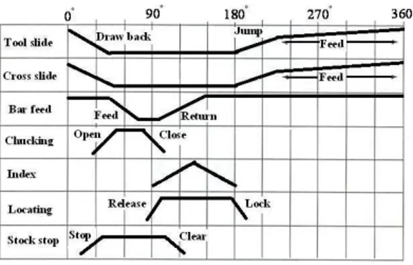
Modeling of the timing diagram is one of the main parts for design of automatic machines. A detailed analysis of the works on the theory of the timing diagram performed prior to 1965 is given in Petrokas (1970). Timing diagram is a sequence of machine operations performed by mechanisms depending on the angular displacement of the main shaft (Browne, 1965; Youssef and El-Hofy, 2008; Homer, 1998; Sandler, 1999; Natale C, 2003; Singh and Bhattacharya, 2006; Levner and Kats, 2007; Niir Board, 2009; Norton, 2009; Topalbekiroglu and Celik, 2009). Timing diagram al-lows determining of the position of each of the executive body at any position of the main shaft (see Fig. 1).

Timing diagram automatic machine is modeled by a di-rected graph (see Fig. 2) (Novgorodtsev, 1982). The disad-vantages of this model are the lack of consideration for con-nections executive bodies displacements mechanisms and ac-counting precision of manufacturing.

Analysis of the methods of synthesis and analysis of tim-ing diagram automatic machine showed the need for further development of optimization methods of timing diagram, taking into account the accuracy of manufacture and the dy-namics of automatic machine.

2 Vector model of the timing diagram of automatic machine

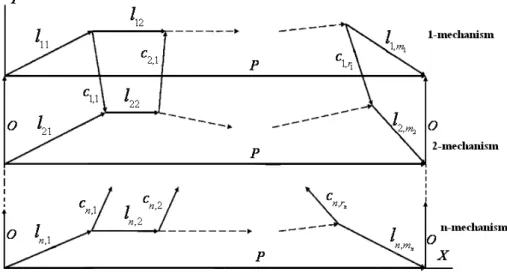
The timing diagram of automatic machines can be repre-sented as the vector polygons (Jomartov, 2010, 2011) (see

Fig. 3). Let us replace the segments linear timing diagram by the vectorsℓ_{i j}_{. The vectors}ℓ_{i j} _{is directed sequentially from}

one position to another position of mechanism, wherei is the number of mechanisms, jis the number of position ofi -mechanism,mjis the number of positions ofi-mechanism,n is the number of mechanisms.

The projection of vectorsℓ_{i j} _{on the}xaxis isαi j – phase angles of actuation of mechanisms. The projectionℓ_{i j}_{on the}

yaxis is the displacementδi jof j-position ofi-mechanism.

δi j =

Si j

Smax

, Smax =maxSi j, i=1, . . . , n; j=1, . . . ,mi,

whereSi jis the displacement ofj-position ofi-mechanism. To explain the parametersαi jandSi jin Fig. 4 shows a dia-gram of the displacement of mechanism, in the figure denote:

αo– phase angles of actuation of mechanism in the position

of open,αdis the phase angles of actuation of mechanism in

the position of dwell,αcis the phase angles of actuation of

mechanism in the position of close,Sois the displacement of

mechanism in the position of open,Scis the displacement of

mechanism in the position of close.

Let us introduce the vector P_{connecting the point of}

be-ginning and end of the cycle. The projection of the vectorP

(2)

392 A. Jomartov: Vector model of the timing diagram of automatic machine

Figure 1.Linear timing diagram of working and auxiliary cams of

a four-spindle bar automatic.

Let us impose the timing diagram of mechanisms at each other using zero vectors (see Fig. 3) connecting the boundary points of timing diagram mechanisms in theyaxis.

Let us compose the system of vector equations describing the works of mechanisms automatic machine (see Fig. 3).

mi

P j=1

ℓ_{i j} ₌ P,i₌1, . . . ,n,

c_ik ₌ n P i=1

mi

P j=1

bi j·ℓi j

             , (1)

wherebi j∈ {0, ±1}.

Let us projected the vector Eq. (1) on the axisxandy.

mi

P j=1

αi j =2π, mi

P j=1

δi j =0,

cx_ik=

n P i=1

mi

P j=1

bi jαi j,c y ik =

n P i=1

mi

P j=1

bi jδi j              (2)

On the phase angles of actuation of mechanismsαi j, and dis-placements of mechanismsδi jimpose constraints

αi j ≥αmi j, δ

ℓ

i j ≥δi j ≥δHi j, (3)

whereαm

i j is the minimum allowable phase angles of actu-ation of mechanisms,δℓ

i j,δ

H

i j is the upper and lower limits assigned by the designer.

On the projection vectors of connection impose constraints

c_ikxℓ ≥c_ikx ≥cx_ikℓ, cyℓ ik ≥c

y ik ≥c

yH

ik (4)

wherecxH

ik =e x ik+ ∆c

x ik,c

yH

ik =e y ik+ ∆c

y

ikwheree x ik,e

y ikare the minimum permissible projection vectors of connection,∆cx

ik, ∆cy

ikare the errors of the projections of vectors of connection, cxℓ

ik,c yℓ

ik are the upper limits imposed by the designer. Equation (2) and constraints (Eqs. 3 and 4) describe the collaboration works of mechanisms (timing diagram) of au-tomatic machine.

Figure 2.Presentation of timing diagram automatic machine as a

directed graph.

3 A mathematical model of automatic machine based on the timing diagram of mechanisms

Lets define the connection between the differential equations of motion the automatic machine and the equations describ-ing its timdescrib-ing diagram. In Fig. 5 shows the dynamic model of the machine, whereci is the elasticity coefficients,βi is the coefficients of resistance,Ji,Iiare the moments of

iner-tia,M∂Bis the motor torque,Miis moment of resistance,Πi,

i=1, . . . ,nis the function of position of mechanisms. To compile the equations of motion mechanisms auto-matic machine (see Fig. 5), let us use Lagrange equations II (Wolfson, 1976):

d dt

∂T

∂ϕ˙j

− ∂T

∂ϕj + ∂V

∂ϕj =Qj+

m P i=1

λihi j

m₊n P j=1

hi jϕ˙j+hi =0,

             (5)

whereϕ1,ϕ2, . . . ,ϕn are the generalized coordinates, λi is Lagrange multipliers,hi j,hiare some functions,T is the ki-netic energy of a holonomic system,Vis the potential energy of the system,Qjis the generalized force.

To establish the connection between the equations of tim-ing diagram (2–4) and the dynamic Eq. (5), let us write the functions of position, the transfer functions of mechanisms of automatic machine in the following form:

Πi= Πi1·1−L(φi−αi1)+ m P

j=2Πi j "

1−L φi− j P

r=1 αir

!# ·L φi−

j−1 P

r=1 αir

!

Π′

i= Π

′

i1 ₁₋_L₍_φ

i−αi1)+ m P j=2Π

′

i j "

1−L φi− j P r=1

αir !#

·L φi− j−1 P r=1

αir !

Π′′

i = Π′′i1 ₁₋_L₍_φ

i−αi1)+ m P j=2Π

′′

i j "

1−L φi− j P r=1

αir !#

·L φi− j−1 P r=1 αir !                            (6)

wherei₌1,. . . . ,n,L(x) is a step function of the form

L(x)=

(

0, x<0,

1, x≥0 .

Πi j,Π′_{i j},Π′′_{i j} are the functions of position, the first transfer function, the second transfer function on parts of phase an-gles of actuationαi jof mechanisms.

(3)

Figure 3.Vector model of the timing diagram of automatic machine.

Figure 4.Diagram of the displacement of mechanism.

method allows to solve various optimization tasks, where the variable parameters are the phase anglesαi j and of the dis-placementsδi jof timing diagram automatic machine.

4 An example

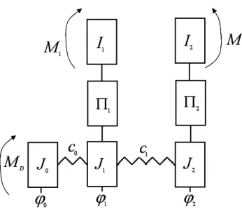
Let us show in more detail the connection between timing diagram of automatic machine and dynamics of mechanisms on the example of automatic machine with two cam mecha-nisms. The dynamic model is shown in Fig. 6, whereϕ0,ϕ1,

ϕ2are generalized coordinates,MDis the motor torque,M1,

M2are the moments of resistance,I1,J0,J1,J2 are the

mo-ments of inertia of mechanisms,c0,c1are the coefficients of

elasticity of shafts,Πi(φi) is the function of position of cam mechanisms,Π′i(φi) is the first transfer functions of the cams, Π′′

i(φi) is the second transfer functions of the cams.

This dynamic model is described by the following equations

J0φ¨0+c1(φ0−φ1)=MD,

J1+I1Π2

′

1(φ1)

¨

φ1+I1Π′1(φ1)Π′′1(φ1) ˙φ21+c0(φ1−φ0)+c1(φ1−phi2)=−M1Π′1(φ1),

J2+I2Π2

′

2(φ2)

¨

φ2+I2Π′2(φ2)Π′′2(φ2) ˙φ22+c2(φ2−φ2)=−M2Π2′(φ₂)

          

(7)

where

Π′i(φi)=

dΠi(φi)

dφi

; Π′′i (φi)=

d2Πi(φi)

dφ2

i

; i=1,2.

Figure 7 shows vector timing diagram of automatic machine, which is described by the following equations:

l₁₁ ₊l₁₂ ₌P l₂₁ ₊l₂₂ ₌P c₂₁ ₌l₂₁ −l₁₁

        

. (8)

Let us projected Eq. (8) on thex,yrespectively

α11+α12 =2π

α21+α22 =2π

cx₁₁ =α21 −α11

        

(9)

δ11−δ12 =0

δ21−δ22 =0

cy₁₁ ₌δ21 −δ11

        

. (10)

Impose the constraints on the phase angles, displacements of mechanisms, and projections of vectors of connection

αi j ≥αmini j δmax

i j ≥δi j ≥δ

min

i j

cx₁₁max ≥cx₁₁ ≥c₁₁xmin

cy₁₁max ≥cy₁₁ ≥cy₁₁min

              

. (11)

The expressions (Eqs. 9–11) allow you to vary the phase angles and displacements of mechanisms of automatic ma-chine, without disrupting their normal work.

(4)

Figure 5.A dynamic model of automatic machine.

Figure 6.Dynamic model of automatic machine with two cams

mechanisms.

Πi= Πi1·1−L(φi−αi1)+ Πi21−L(φi−(αi1+αi2))·L(φi−αi1) Π′

i= Π

′

i1· ₁₋_L₍_φ

i−αi1)+ Π′i2 ₁₋_L₍_φ

i−(αi1+αi2))·L(φi−αi1) Π′′

i = Π

′′

i1· ₁₋_L₍_φ

i−αi1)+ Π′′i2 ₁₋_L₍_φ

i−(αi1+αi2))·L(φi−αi1)         

i₌1,2

(12)

where

L(x)=

(

0, x<0,

1, x≥0. .

Represent the generalized coordinatesϕ1,ϕ2through the

di-mensionless coefficientsk1,k2whereϕ1=2πk1;ϕ2=2πk2;

k1,k2∈[0, 1]

Figure 7.Vector timing diagram of automatic machine with two

cams mechanisms.

Πi j =ai j(ki)δi j Π′i j =bi j(ki)

δi j αi j

Π′′i j =di j(ki)

δi j α2 i j

            

i =1, 2; j=1,2

. (13)

ai j(ki),bi j(ki),di j(ki);i=1, 2; j=1, 2; are coefficients of the displacement, the velocity, the acceleration of mechanism in

j-position.

(5)

Figure 8.The functions of position and the transfer functions of mechanisms of automatic machine.

varying the parameters of timing diagram αi j and δi j, can improve the dynamics of the automatic machine. As an opti-mization criterion can use the following expression:

max

ϕi Π ′

i(ϕi)Π′′i (ϕi).

5 Conclusions

The vector model of timing diagram is developed on the basis of representation timing diagram of the automatic machine as vector polygons, which allows solving various dynamic tasks at the expense of change of parameters of timing diagram.

The mathematical model of the automatic machine with elastic links on the basis of the timing diagram of its mecha-nisms is received.

The equations of connection between parameters timing diagram of the automatic machine and equations of dynam-ics through functions of position and transfer functions of mechanisms were received.

The model of timing diagram of the automatic machine is the only method which allows to solve a variety of dynamic tasks, by optimizing its timing diagrams, at this time.

Edited by: A. Barari

Reviewed by: two anonymous referees

References

Browne, J. W.: The Theory of Machine Tools, Cassell and Co. Ltd., London, p. 374, 1965.

Homer, D. E.: Kinematic Design of machines and mechanisms, McGraw-Hill, New York, p. 661, 1998.

Jomartov, A.: Dynamics of machine-automaton jointly with cycle-gram, World Congress on Engineering, Lîndon, UK, 1224–1229, 2010.

Jomartov, A.: Multi-Objective Optimization Of Cyclogram Mech-anisms Machine-Automaton, World Congress on Engineering, Lîndon, UK, 2562–2565, 2011.

Levner, E. and Kats, V. D.: Cyclic Scheduling in Robotic Cells:An Extension of Basic Models in Machine Scheduling Theory, Mul-tiprocessor Scheduling: Theory and Applications, Vienna, Aus-tria, p. 436, 2007.

Natale, C.: Interaction control of robot manipulators: six degrees-of-freedom tasks, Springer-Verlag, Berlin, p. 108, 2003. Niir Board: Complete technology book on textile, spinning,

(6)

Norton, R. L.: Cam Design and Manufacturing Handbook, Indus-trial Press Inc., p. 591, 2009.

Novgorodtsev, V. A.: Presentation of the machine timing diagram as a graph, Theory of mechanisms and machines, Kharkov, 33, 57–60, 1982.

Petrokas, L. V.: Reviews of timing diagram manufacturing ma-chines and automatic production lines, J. Theory of automatic machines and pneumatic, Moscow, 22–36, 1970.

Sandler, B. Z.: Robotics: designing the mechanisms for automated machinery, Academic Press, San Diego, p. 433, 1999.

Singh, B. and Bhattacharya, S. K.: Control of machines, New Age International, New Delhi, p. 338, 2006.

Topalbekiroglu, M. and Celik, H. I.: Kinematic analysis of beat-up mechanism used for handmade carpet looms, Indian J. Fibre Textile Res., 34, 129–136, 2009.

Wolfson, I. I.: Dynamics calculations of cycle mechanisms, Mashinostroenie, Leningrad, p. 328, 1976.