www.ann-geophys.net/32/793/2014/ doi:10.5194/angeo-32-793-2014
© Author(s) 2014. CC Attribution 3.0 License.
Cloud radiative forcing intercomparison between fully coupled
CMIP5 models and CERES satellite data
M. Calisto1, D. Folini2, M. Wild2, and L. Bengtsson1 1International Space Science Institute (ISSI), Bern, Switzerland
2Institute for Atmospheric and Climate Science ETH, Zurich, Switzerland
Correspondence to:M. Calisto ([email protected])
Received: 31 October 2013 – Revised: 26 March 2014 – Accepted: 10 June 2014 – Published: 17 July 2014
Abstract.In this paper, radiative fluxes for 10 years from 11 models participating in the Coupled Model Intercomparison Project Phase 5 (CMIP5) and from CERES satellite obser-vations have been analyzed and compared. Under present-day conditions, the majority of the investigated CMIP5 mod-els show a tendency towards a too-negative global mean net cloud radiative forcing (NetCRF) as compared to CERES. A separate inspection of the long-wave and shortwave con-tribution (LWCRF and SWCRF) as well as cloud cover points to different shortcomings in different models. Mod-els with a similar NetCRF still differ in their SWCRF and LWCRF and/or cloud cover. Zonal means mostly show ex-cessive SWCRF (too much cooling) in the tropics between 20◦S and 20◦N and in the midlatitudes between 40 to 60◦S.
Most of the models show a too-small/too-weak LWCRF (too little warming) in the subtropics (20 to 40◦
S and N). Dif-ference maps between CERES and the models identify the tropical Pacific Ocean as an area of major discrepancies in both SWCRF and LWCRF. The summer hemisphere is found to pose a bigger challenge for the SWCRF than the win-ter hemisphere. The results suggest error compensation to occur between LWCRF and SWCRF, but also when taking zonal and/or annual means. Uncertainties in the cloud radia-tive forcing are thus still present in current models used in CMIP5.
Keywords. Meteorology and atmospheric dynamics (clima-tology; radiative processes; instruments and techniques)
1 Introduction
The sun is the most important energy source for the planet earth. Its energy is the main driver of earth’s dynamics, which involve winds, ocean currents, evaporation/precipitation, etc. It is therefore a basic prerequisite that the amount of solar energy received from the sun, and the amount that is re-flected and radiated back from our planet, are adequately represented in models so that the earth’s energy budget is correctly represented.
The earth’s energy budget is approximately in equilibrium as seen over the past few years and over the entire earth, i.e., the outgoing long-wave radiation nearly balances the incom-ing absorbed shortwave radiation.
Clouds have a strong impact on the radiation budget of the earth. They increase the global reflection 15–30 % (e.g., Wild et al., 2013), causing the albedo of the entire earth to be about twice of what it would be in the absence of clouds (Cess, 1976). Clouds also absorb the long-wave radiation emitted by the earth’s surface and emit energy into space at the tem-perature at the cloud tops (e.g., Ramanathan et al., 1989).
Cloud forcing thus is negative for the shortwave component, where clouds generally have a cooling effect, and positive for the long-wave component, where clouds generally have a warming effect. A recently published paper by Probst et al. (2012) shows that the global mean cloud fraction (CF) in the CMIP3 models, averaged from January 1984 to De-cember 1999, exhibits a considerable variance and generally underestimates the CF as given by the International Satellite Cloud Climatology Project (ISCCP) D2 data set in a latitu-dinal belt from 60◦
S to 60◦
N (see Fig. 1 in Probst et al., 2012). Ichikawa et al. (2012) used ISCCP and Earth Radi-ation Budget Experiment (ERBE) observRadi-ations to evaluate the CRF over tropical convective regions for CMIP3 mod-els. They showed that most of the models systematically overestimate the shortwave CRF and underestimate the long-wave CRF over regions with weak vertical motion. Wang and Su (2013) compared CMIP5 atmospheric general circula-tion model (AGCM) data with CERES Energy Balance And Filled (EBAF) satellite data and demonstrated that modeled CRF shows the same deficiencies as presented in Ichikawa et al. (2012). In addition, they pointed out that models strongly underestimate shortwave cloud radiative forcing (SWCRF) over the subtropical stratocumulus region, while long-wave cloud radiative forcing (LWCRF) is strongly underestimated in regions of strong subsidence. Comparing CMIP3 and CMIP5 data with CERES EBAF, Li et al. (2013) found a persistent systematic underestimation (overestimation) of re-flected radiative shortwave (long-wave) upward flux at TOA over convectively active tropical regions. Trenberth and Fa-sullo (2010) showed that CMIP3 models have a positive bias in the absorbed solar radiation over the surface of the South-ern Ocean (between 45 and 60◦S) which is most likely due to
an underestimation of the cloud amount. Wild (2008) came to the conclusion that the IPCC-AR4/CMIP3 models show a tendency to overestimate the downward solar radiation and underestimate the downward long-wave radiation at the sur-face. Wild et al. (2013) found that the IPCC-AR5/CMIP5 models still show a similar uncertainty range on the order of 10 W m−2for the major surface energy balance components, as well as a tendency to overestimate the downward solar ra-diation and underestimate the downward thermal rara-diation, respectively.
Uncertainties in CRF can have far reaching consequences. For example Ceppi et al. (2012) analyzed CMIP5 data, find-ing that a substantial fraction of the biases in the latitudinal position of the jet can be explained by anomalies in midlati-tude (40 to 60◦S) shortwave forcing due to clouds, meaning
that models with anomalously negative cloud shortwave forc-ing tend to exhibit an equatorward bias in jet latitude. Huber et al. (2011), analyzing the constraints on climate sensitiv-ity from radiation patterns in climate models, state that the LWCRF and the SWCRF show a high positive and negative correlation with the total cloud amount and the atmospheric water vapor. This implies that having a radiative balance
different from reality is likely accompanied by a bias in the above mentioned species.
In this study, we focus on the intercomparison of CMIP5 models and observational data from the Clouds and the Earth’s Radiant Energy System (CERES, Wieliecki et al., 1996), with an emphasis on cloud radiative forcing. Our goal is to compare CMIP5 models and the satellite data from CERES to quantify differences in the CRF at the top of the atmosphere, from the global to regional scale, and to ana-lyze potential differences between the model and the satellite data.
Section 2 describes the data and the methods used in this paper, Sects. 3 and 4 provide the results and a summary with an outlook, respectively.
2 Data and methods
The CERES instrument is designed to provide a climate data set suitable for examining the role of clouds in the radiative balance of the climate system. CERES is able to measure the thermal radiation emitted from the earth’s surface in the 8–12 µm window. The two other CERES spectral bands mea-sure shortwave (0.2–5 µm) and total (0.2–100 µm) broadband radiation. Broadband long-wave radiation is estimated as the total minus shortwave radiation. Satellite overpass output products are given at the CERES field of view resolution (20 to 50 km), while all 3 h synoptic, daily, monthly, and yearly average products are made available on the CERES equal-area (140 km×140 km) grid (Wielicki et al., 1995). Further details about CERES can be found in Wielicki et al. (1995). In the present work, the monthly mean TOA radiative fluxes of CERES for the shortwave and long-wave cloud radiative forcing are used, derived from Level 4 EBAF Ed2.6r prod-ucts with a global grid resolution of 1◦
×1◦
for 10 years (2000 to 2010) (Loeb et al., 2009). For the cloud area frac-tion, the CERES SYN1deg Ed2.6 (Minnis et al., 2011) data has been used. Stubenrauch et al. (2013) stated in their paper that CERES, compared to the other satellite-derived data sets in their paper, shows a total cloud amount that is lower than the mean of the satellites analyzed in their paper.
upward radiation data has been used to calculate the CRF, i.e., we have subtracted the all-sky data from the clear-sky data for a 10-year period (1995 to 2005) of the all forcings experiments. Since CERES data is only available from 2000 to 2010, and while all the CMIP5 models participating in the historical experiments end in 2005, the authors decided to compromise on the period (2000 to 2010 for CERES, 1995 to 2005 for the model data) instead of using model data from different experiments (historical until 2005 plus some sce-nario later on) for their paper. The same procedure is done by Ceppi et al. (2012), who also used different time frames, i.e., CERES from 2000–2010 and 1979–2005 for the model data. Since the climate model simulations are not determinis-tic, such slight shifts in the analyzed period do not introduce any relevant additional biases. In this study, we compare the CERES data directly with the model data (see results sec-tion). We note, however, that more elaborate techniques us-ing simulators exist (e.g., Bodas-Salcedo et al., 2011; Webb et al., 2001).
The list of the CMIP5 models used here is given in Table 3. We follow the practice adopted by other authors (e.g., Lauer and Hamilton, 2013; Li et al., 2013; and Ceppi et al., 2012) and examine only one ensemble member (r1i1p1). Quantify-ing differences between ensemble members for all the mod-els and quantities considered here, and ranging from global means to seasonal maps, is beyond the scope of this paper. We note, however, that at least for the global mean values of the components of the earth’s radiative energy balance, Wild et al. (2013) indeed found differences between models to be much larger than differences between ensemble members of the same model. For comparison with CERES data (see Figs. 2–4), the CMIP5 data were remapped onto the CERES grid. The focus in this paper is placed more on the geograph-ical and seasonal distribution of differences between model and CERES data than on the physical interpretation of the differences.
3 Results 3.1 Global mean
The global mean cloud radiative forcing averaged over 10 years for the CMIP5 models as well as for CERES satel-lite data is given in Table 1. The values in parentheses show the minimum and the maximum anomaly of the yearly values from the 10-year mean.
According to Table 1, the global mean long-wave cloud radiative forcing for the CMIP5 models out of Table 3 spans from 20.7 to 30.7 W m−2, whereas the shortwave cloud ra-diative forcing spans from−40.8 to−54.7 W m−2. The long-wave cloud radiative forcing (LWCRF) and the shortlong-wave cloud radiative forcing (SWCRF) given by CERES are 29.5 and −47.5 W m−2, respectively. Comparing these results, one can see that the majority of the CMIP5 models (7 out of
the 11 models) have a too-strong, too-negative SWCRF. The LWCRF is too weak for most of the models (9 out of the 11 models), which indicates not enough warming of the planet due to LWCRF. The net cloud radiative forcing (NetCRF) given by the CMIP5 models is lower (more negative) in 11 out of 11 models than the results depicted by the satellite, with values spans from−19.9 to−28.9 W m−2as compared to the CERES value of−18 W m−2(see Table 1).
From Table 1 it can be further interpreted that nearly the same NetCRF can be obtained for largely different global cloud amounts. Several other papers, for example Zhang et al. (2005) and Klein et al. (2013), have also shown that mod-els may not have the same cloud amount, yet have a CRF that fits well with the satellite data. Klein et al. (2013), for example, state in their paper that even though the global an-nual average of the top-of-the-atmosphere NetCRF is close to zero compared to the satellite data, significant regional errors in the radiation field may persist. They also point out that one common error is having lower-than-observed cloud amounts with larger-than-observed values of the optical cloud thick-ness.
Specific model pairs displaying this behavior are CCSM4 and CanESM2, as well as GFDL and bcc-csm1 (both having nearly the same NetCRF but a widely different cloud cover). The first pair, moreover, even have nearly identical SWCRF and LWCRF, despite widely different cloud cover. A third set of models with nearly identical NetCRF but different cloud cover, LWCRF, and SWCRF are ACCESS 1-0, inmcm4, and IPSL-CM5A-LR. These findings indicate compensation of errors within single models on the global scale. Potential rea-sons why nearly the same NetCRF is obtained for widely dif-ferent cloud cover include difdif-ferent cloud heights in the mod-els (Zelinka et al., 2012), different optical properties (Zelinka et al., 2012; Zhang et al., 2005; Klein et al., 2013) of the cloud droplets, or differences in the radiative transfer mod-eling (Collins et al., 2006). Collins et al. (2006), focusing on the forcing by well-mixed greenhouse gases in their ra-diative transfer model intercomparison, state that there are differences in the treatment of the radiative transfer among the models investigated in their paper, which might be one of the reasons for the different results mentioned in the above paragraph.
Having seen that globally, most CMIP5 models have a too-negative (cooling) CRF, we next turn to zonal means to iden-tify particularly susceptible latitudinal bands.
3.2 Zonal mean
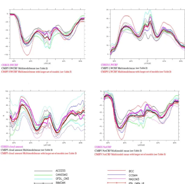
Figure 1 shows a 10-year average zonal mean for the SWCRF (upper left), LWCRF (upper right), NetCRF (lower right), all given in W m−2; and total cloud amount (CLT; lower left, given in percent) for the CERES data and two multi-model means, for a set of 30 CMIP5 models (see Table 3).
Table 1.Global mean radiative forcing for the CMIP5 models and CERES satellite data averaged over 10 years. The abbreviation rlut stands for long-wave upward all-sky radiation at the top-of-the-atmosphere and rlutcs for clear-sky instead of all-sky. The abbreviations rsut and rsutcs are the same for shortwave radiation, respectively. Numbers in parentheses represent the minimum and maximum anomaly from the 10-year means compared with yearly values.
rlutcs rlut LWCRF rsutcs rsut SWCRF clt NetCRF
Model [W m−2] [W m−2] [W m−2] [W m−2] [W m−2] [W m−2] [%] [W m−2]
ACCESS1-0 266.9 241.7 25.2 (+0.16;−0.34) 53.7 98.8 −45.1 (+0.81;−1.35) 53.8 −19.9 (+0.95;−1.22) bcc-csm1 262.5 235.5 27 (+0.18;−0.38) 49.8 103.3 −53.5 (+0.57;−0.82) 57.8 −26.5 (+0.38;−0.65) CanESM2 265 239.7 25.3 (+0.3;−0.04) 53.5 100.7 −47.2 (+1.27;−0.79) 60.9 −21.9 (+1.43;−0.75) CCSM4 265.4 240.1 25.3 (+0.38;−0.36) 50.3 97.4 −47.1 (+1.23;−0.44) 46.3 −21.8 (+1.61;−0.43) GFDL 261.4 235.2 23.8 (+0.87;−0.59) 53.7 104.2 −50.4 (+2.56;−1.37) 72.1 −26.6 (+3.43;−1.78) HadCM3 260.5 239.3 21.2 (+0.68;−0.64) 51.5 101.6 −50.1 (+0.54;−0.37) 47.7 −28.9 (+0.79;−1.03) inmcm4 264.1 243.4 20.7 (+0.37;−0.53) 56 96.8 −40.8 (+0.65;−0.64) 63.4 −20.1 (+0.49;−0.4) IPSL-CM5A-LR 268.1 237.5 30.7 (+0.37;−0.27) 51.8 103.2 −51.4 (+0.73,−0.26) 57.2 −20.7 (+0.75;−0.87) MIROC5 261 234.8 26.1 (+0.75;−0.27) 50.4 105.1 −54.7 (+0.87;−0.92) 56.8 −28.6 (+0.62;−0.35) MPI-ESM-P 261.5 236.7 24.8 (+0.32;−0.25) 53.8 102.2 −48.4 (+1.97;−0.29) 62.7 −23.6 (+0.94;−0.34) Nor-ESM1-ME 261.6 232 29.6 (+0.71;−0.38) 51.2 105.6 −54.4 (+0.64;−0.43) 53.7 −24.8 (+0.42;−0.48) CERES (satellite) 268.4 238.9 29.5 (+0.31;−0.36) 52.4 99.6 −47.5 (+0.33;−0.48) 61.3 −18 (+0.25;−0.84)
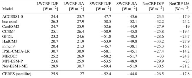
Table 2.Global mean LWCRF, SWCRF, and NetCRF for DJF and JJA for several CMIP5 models as well as for CERES satellite data averaged over 10 years.
LWCRF DJF LWCRF JJA SWCRF DJF SWCRF JJA NetCRF DJF NetCRF JJA Model [W m−2] [W m−2] [W m−2] [W m−2] [W m−2] [W m−2] ACCESS1-0 24.4 25.7 −47.7 −43.6 −23.3 −17.9 bcc-csm1 26.3 27.9 −58.5 −52.1 −32.2 −24.2 CanESM2 24.7 25.9 −52.6 −44.9 −27.9 −19 CCSM4 25.1 26.4 −50.9 −45.8 −25.8 −19.4 GFDL 23.2 24.6 −51.8 −48.3 −28.6 −23.7 HadCM3 20.7 21.9 −53.9 −49.8 −33.2 −27.9 inmcm4 20.4 21.3 −45.7 −38.1 −25.3 −16.8 IPSL-CM5A-LR 30.7 30.9 −58.1 −45.1 −27.4 −14.2 MIROC5 25.2 26.9 −58.2 −51.7 −33 −24.8 MPI-ESM-P 23.6 25.9 −53.5 −48.9 −29.9 −23 Nor-ESM1-ME 28.9 30.7 −59.4 −51.9 −30.5 −21.2
CERES (satellite) 25.9 27 −52.4 −44.8 −26.5 −17.8
set of 30 CMIP5 models for all four variables considered here. In this sense, our selection of 11 models is represen-tative. Moreover, these 11 models are a representative selec-tion out of the models in Table 3. They cover, at least for the global mean values, the range of the models mentioned in Table 3.
The multi-model means, given as thick lines, show a better agreement with the satellite data than each single model run separately. This may be seen as error compensation across models when taking the multi-model mean. On the level of individual models, comparison of Fig. 1 with Table 1 shows that a comparatively good global mean value (e.g., NetCRF of−19.9 W m−2in the ACCESS1-0 model) can be obtained despite substantial deficiencies of zonal means.
The multi-model mean NetCRF deviates particularly strongly from CERES between around 50◦
S and 50◦
N. Looking separately at LWCRF and SWCRF reveals that this
too-negative NetCRF is due to too little (warming) LWCRF between 20 and 40◦ (N and S) and a narrow band around
5◦N, as well as due to too much (cooling) SWCRF in the
tropics (20◦S to 20◦N). In a region from 65◦S to 65◦N,
cloud cover is essentially underestimated everywhere, except slightly south and north of the equator. Overall, it can be said that the zonal mean analysis shows that for the multi-model means, the largest biases for the CRF between the modeled data and CERES are in the equatorial tropical region (20◦
S to 20◦
N). Essentially all the models, except for the IPSL-CM5A-LR model, have a too-negative NetCRF in this lati-tudinal band as compared to CERES. This finding is in line with results by Nam et al. (2012). They found that in the tropical region (30◦
S to 30◦
Figure 1.SWCRF and LWCRF (upper left and upper right) given in W m−2, cloud amount (lower left) given in percent and NetCRF (lower right) given in W m−2for the models listed in Table 4 together with CERES data and the multi-model zonal mean for 10 years.
in concert with the results depicted in Wang and Su (2013), i.e., both studies conclude that CMIP5 models produce less cloud amounts than observed, and that the good results in CRF are due to compensating errors. They state, furthermore, that over subtropical subsidence regions a weaker SWCRF is visible, similar to what is seen in our results.
3.3 Global maps
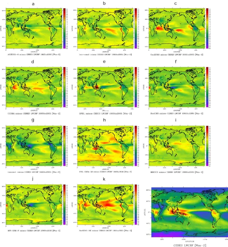
To further assess the differences between the CMIP5 data and CERES, we check whether the differences can be attributed to specific regions. For this, we look at each model sepa-rately, comparing it to the satellite data for the same variables already displayed in Fig. 1. We consider again a 10-year mean, but this time look at global maps. Figures 2–4 show LWCRF, SWCRF, and the total cloud amount. Panels a–k show the difference between the specific CMIP5 model and
the CERES data. The lower part of each panel shows the zonal means for both data sets’ 10-year mean, again. The CERES data, averaged over 10 years, is shown in the low-ermost right corner of each figure. All the data for the cloud radiative forcing are given in W m−2, the plots for the cloud amount are given in percent. Note that satellites may have problems in the polar regions retrieving the correct result cause the instruments may have problems distinguishing be-tween clouds and ice cover. Therefore, we have to be cautious when looking at high-latitude/ice-covered regions.
Figure 2.Long-wave cloud radiative forcing (LWCRF) for CERES and several CMIP5 models. Panels(a)to(k)show map plots for the specific CMIP5 models minus CERES data. In the lowermost right corner is the CERES LWCRF plot. All plots are given in W m−2 representing a 10-year mean. The color bar for the CERES LWCRF plot: −6 up to 70 W m−2and for the difference plots:−52 up to 42 W m−2.
another reason for these deviations is suggested in Mechoso et al. (1995) and Michael et al. (2013), the latter authors studying the CMIP5 models. They found that the majority of the CMIP5 models exhibit cold biases in sea surface tempera-ture in equatorial oceans, which is redolent of an Intertropical
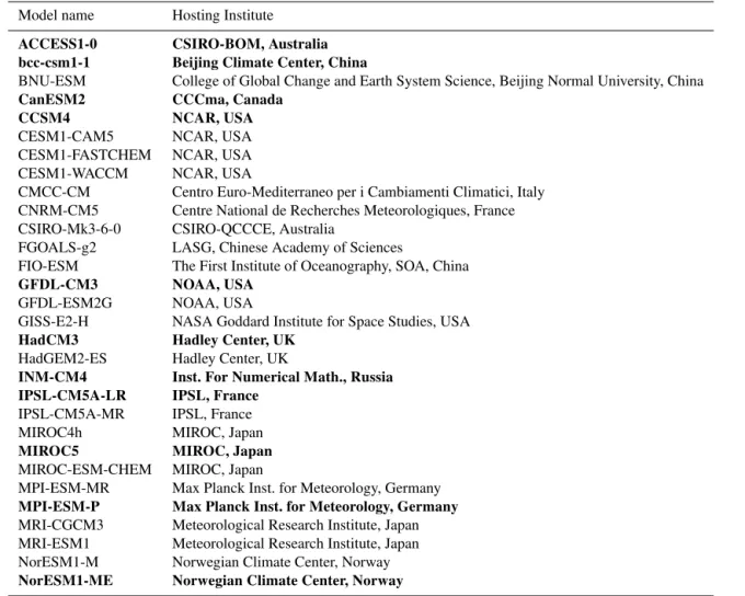
Table 3.List of CMIP5 models used for the “Multi-model mean larger set of models” plot in Fig. 1. CMIP5 models in bold font are the models used for the rest of the plots.
Model name Hosting Institute
ACCESS1-0 CSIRO-BOM, Australia bcc-csm1-1 Beijing Climate Center, China
BNU-ESM College of Global Change and Earth System Science, Beijing Normal University, China CanESM2 CCCma, Canada
CCSM4 NCAR, USA
CESM1-CAM5 NCAR, USA CESM1-FASTCHEM NCAR, USA CESM1-WACCM NCAR, USA
CMCC-CM Centro Euro-Mediterraneo per i Cambiamenti Climatici, Italy CNRM-CM5 Centre National de Recherches Meteorologiques, France CSIRO-Mk3-6-0 CSIRO-QCCCE, Australia
FGOALS-g2 LASG, Chinese Academy of Sciences
FIO-ESM The First Institute of Oceanography, SOA, China GFDL-CM3 NOAA, USA
GFDL-ESM2G NOAA, USA
GISS-E2-H NASA Goddard Institute for Space Studies, USA HadCM3 Hadley Center, UK
HadGEM2-ES Hadley Center, UK
INM-CM4 Inst. For Numerical Math., Russia IPSL-CM5A-LR IPSL, France
IPSL-CM5A-MR IPSL, France MIROC4h MIROC, Japan MIROC5 MIROC, Japan MIROC-ESM-CHEM MIROC, Japan
MPI-ESM-MR Max Planck Inst. for Meteorology, Germany MPI-ESM-P Max Planck Inst. for Meteorology, Germany MRI-CGCM3 Meteorological Research Institute, Japan MRI-ESM1 Meteorological Research Institute, Japan NorESM1-M Norwegian Climate Center, Norway NorESM1-ME Norwegian Climate Center, Norway
underestimated (bluish) by the models. In fact, the multi-model zonal means (Fig. 1) show mostly good agreement with the CERES data in the tropics. Compared with CERES, the model from France, IPSL-CM5A-LR, is the only one showing higher zonal mean values in the LWCRF all the way from the southern polar region up to the northern po-lar region. From Fig. 2h, it can be further interpreted that this overestimation is not restricted to any particular longitude but is rather global in nature.
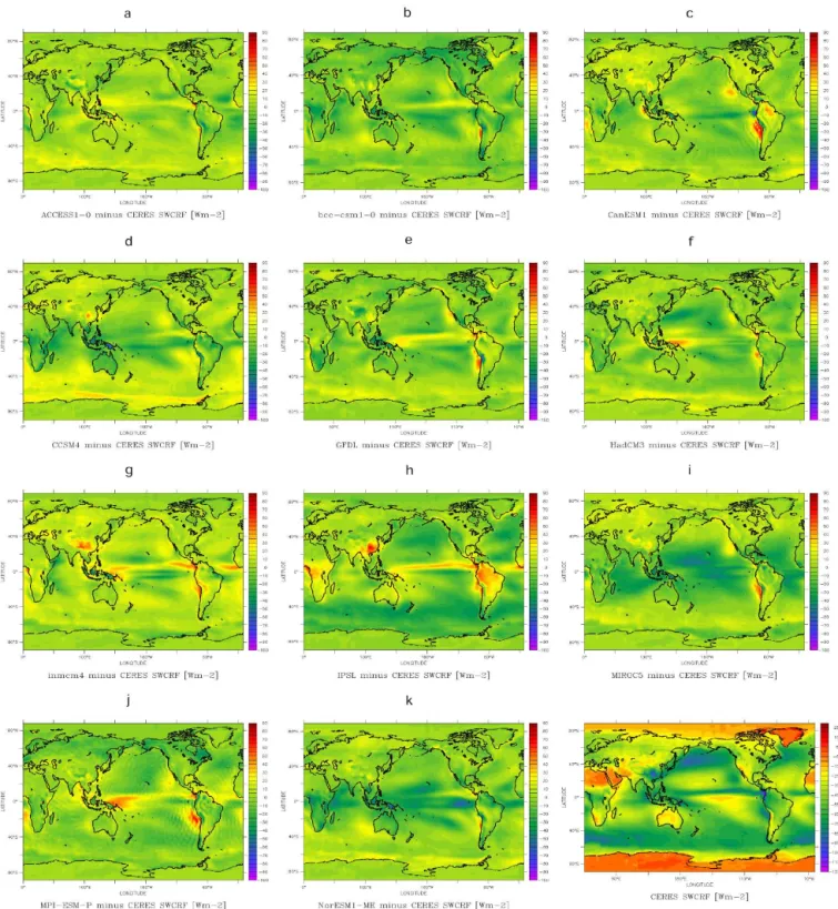
The SWCRF in Fig. 3 shows an overall similar picture, except that the sign of the model deviation with respect to CERES is more consistent across models: SWCRF is mostly stronger (bluish) in the models, which carries over to the multi-model zonal mean shown in Fig. 1. The dip in SWCRF in the Pacific just north of the equator is missed by a number of models. Also clearly apparent is the underestimation in subtropical stratocumulus regions off the west coast of South America and, to a lesser degree, North America and South Africa, a well known deficiency of global climate models
(also, see for example the recent publications by Lauer and Hamilton, 2013, and by Wang and Su, 2013).
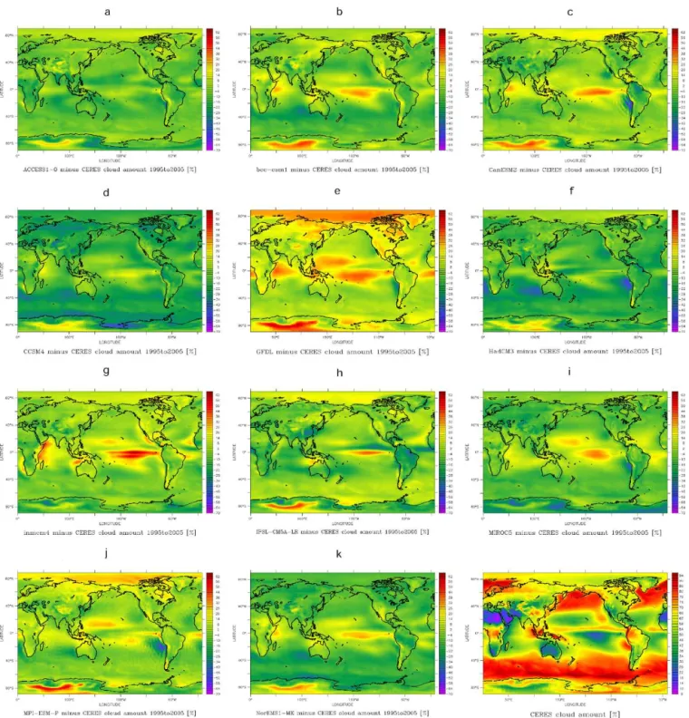
Regarding the total cloud amount (Fig. 4) some of the models show substantial differences compared to CERES observations. The differences are not only visible over the equatorial region; they are also visible throughout the whole globe. Most of the models simulate less cloud amounts than seen in the satellite data. Interestingly, some CMIP5 models change to an overestimation around the equator where the ENSO region is situated. Zhang and Jin (2012) demonstrated the existence of a systematical narrow bias in the simulated ENSO meridional width for sea surface temperature anomaly in CMIP5, i.e., the models show less intense precipitation in this region leading to more clouds. Bellenger et al. (2014) also identifies that the precipitation over the equatorial Pa-cific is poorly represented in the CMIP5 models, showing that the models still struggle to represent cloud processes.
Figure 3. Shortwave cloud radiative forcing (SWCRF) for CERES and several CMIP5 models. Panels(a)to (k)show a map plot for the specific CMIP5 model minus CERES data. In the lowermost right corner is the CERES SWCRF plot. All plots are given in W m−2 representing a 10-year mean. The color bar for the CERES SWCRF plot:−125 up to 25 W m−2and for the difference plots:−100 up to 90 W m−2.
in cloud amount and deviations in either SWCRF or LWCRF. For example, cloud cover is overestimated over wide ar-eas by the GFDL model but severely underestimated by the
Figure 4.Total cloud amount (CLT) for CERES and several CMIP5 models. Panels(a)to(k)show a map plot for the specific CMIP5 model minus CERES data. In the lowermost right corner is the CERES CLT plot. All plots are given in percent representing a 10-year mean. The color bar for the CERES CLT plots: 4 up to 100 % and for the difference plots:−70 up to 65 %.
the cloud cover gives a bigger bias than the SWCRF or the LWCRF compared to satellite data, has also been found in Lauer and Hamilton (2013). They state, that the reason why the LWCRF and the SWCRF fit better to observations is because these variables affect directly the global mean radiative balance of the earth. Therefore, model develop-ers may focus on the tuning of these variables (Lauer and
3.3.1 Seasonal maps
In this subsection, we check whether the differences between CMIP5 data and satellite data are more pro-nounced when looking at different seasons, i.e., Decem-ber/January/February (DJF) and June/July/August (JJA), again for 10-year means. We start with a look at Table 2, where seasonal cloud radiative forcing values are given for the different models. The absolute value for global NetCRF is larger during DJF than during JJA, in concert with the larger TOA incoming values during winter, when the earth is closer to the sun. Differences in NetCRF between DJF and JJA tend, however, to be smaller in the models than what is observed by CERES. Also, interestingly Table 2 shows that on the sea-sonal level there exist models whose NetCRF is less negative than the CERES data (three in DJF, two in JJA). This con-trasts with all models having a too-strong NetCRF as com-pared to CERES if the annual mean is considered. For the LWCRF and SWCRF, the overall picture is similar for JJA and DJF than in the annual mean: 3 out of 11 models under-estimate the LWCRF, both in JJA and DJF, while 2 out of 11 models underestimate the SWCRF, again for both seasons.
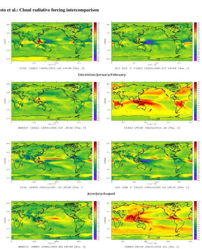
To get a better idea of the geographical origin of the dif-ferences between models and observations, we look again at maps. Even though we analyze all the models given in bold font out of those in Table 3, three models from the list, repre-senting a selection from different countries and different res-olution, are taken as examples (GFDL, MIROC5 and MPI-ESM-P), subtracting the CERES data from the modeled data. The results of this comparison are presented in Figs. 5 and 6. The four upper panels of Fig. 5 show the differences for the long-wave cloud radiative forcing as compared to CERES in W m−2for DJF, as well as the absolute CERES values. The four lower panels show the same quantities for JJA.
Looking first at LWCRF during the Northern Hemi-spheric winter, i.e., DJF (upper part Fig. 5), large differ-ences compared to CERES are visible in the equatorial Pa-cific and northeast of Australia, especially for the MPI-ESM-P model, depicting the largest underestimation of more than 45 W m−2. The Southern Hemisphere, the summer hemi-sphere during DJF, shows almost no bias; the only excep-tions are seen in the GFDL and the IPSL-CM5A-LR (not shown) model. There, we see an overestimation over Antarc-tica and northwest of Australia of about 20 W m−2and up to 40 W m−2, respectively.
The plots for JJA (lower part Fig. 5) show larger differ-ences compared to the satellite data. In all the models, one re-gion is clearly visible in a latitudinal band from about 20◦
N to 20◦
S. There, the models show a more pronounced over-estimation, up to 45 W m−2compared to the satellite data in the Pacific. Three of the models, the MPI, GFDL, and in-mcm4 (not shown) show a negative bias around the equa-torial Pacific. The other region where all models show a positive bias is at the coast of Antarctica. A potential ex-planation here may be a different representation of sea ice
among the models which has also been noted by Turner et al. (2013), who said that the sea-ice extent over Antarctica has not been represented correctly over the last 27 years. The CMIP5 models show a negative trend while the observations show an increase over the last 30 years. Yamanouchi and Charlock (1997) show in their paper that a smaller sea-ice extent leads predominantly to a smaller albedo which leads then to more long-wave emission, giving rise to an increase in the LWCRF. The overestimation is less pronounced than in the above mentioned latitudinal band but still visible.
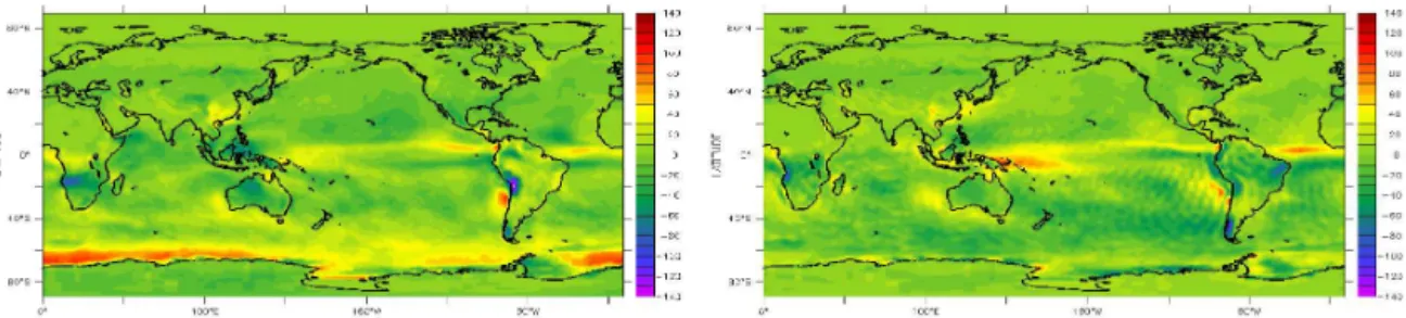
Turning now to SWCRF, Fig. 6, one can see that differ-ences are generally more pronounced in the summer hemi-sphere than in the winter hemihemi-sphere. The largest differences occur over the continents and at the coastal regions. The GFDL model depicts the highest overestimation at the coast of Antarctica of up to 100 W m−2, whereas the MPI and the IPSL-CM5A-LR models (not shown) show a slight underes-timation in the same region, which again might be due to a different representation of the sea ice in this region. Overall it can be said that the Southern Hemisphere during DJF shows more differences than seen in the Northern Hemisphere dur-ing the same time.
The plots for JJA, presented in the lower part of Fig. 6, show for the Northern Hemisphere that these three models (as well as the other models, not shown) underestimate the SWCRF by up to 60 W m−2over the Pacific and the Atlantic in a latitudinal band from 10 up to 60◦
N. The biases over land are mostly positive except the MPI-ESM-P and the bcc-csm1 models (not shown), showing a negative bias with a maximum of approximately 80 W m−2over the eastern part of Canada and Alaska in the MPI model. During the same months, all the models depict that the Southern Hemisphere shows a better agreement than seen in the Northern Hemi-sphere. The models show that the equatorial region in the Pa-cific and the west coast of South America depict an overes-timation of up to 60 W m−2. MIROC5 as well as NorESM1-ME (not shown) show a negative bias of up to 30 W m−2 from the equator down to approximately 20◦
S. The seasonal analysis shown in Figs. 5 and 6 reveals that for the SWCRF the CMIP5 models are closer to CERES data in the winter hemisphere. This cannot be said for the LWCRF, where the results are more ambiguous.
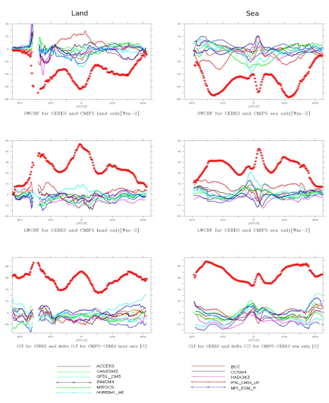
3.3.2 Sea/Land maps
Figure 5.Seasonal plots showing the difference between CMIP5 and CERES for LWCRF for 10 years for MPI-ESM-P, MIROC5, and GFDL, as well as LWCRF observed by CERES. The upper four panels show DJF, lower four panels JJA. Plots show results given in W m−2.
amount. The plots depict differences between the modeled data and the satellite data for a 10-year annual mean as well as absolute values from CERES given as a starred line. The results for the CRF are given in W m−2. Results for the cloud amount are given in percent.
From Fig. 7 it can be interpreted that the line plots, repre-senting the differences between the models and the satellite data for SWCRF, tend to be closer to each other over land than over sea, especially in the Southern Hemisphere. An
Figure 6.Seasonal plots showing differences between CMIP5 and CERES for SWCRF for 10 years for MPI-ESM-P, MIROC5, and GFDL. The upper panel shows DJF, lower panel JJA. Plots show results given in W m−2.
negative, whereas over sea the models show a more equal distribution, i.e., about one half have a positive bias and the other half show a negative bias seen over both hemispheres. Finally, the difference plots for the total cloud amount shows, on the one hand, that the CMIP5 models mostly underesti-mate the total cloud amount in both hemispheres and, on the other hand, that models start to diverge strongly among them-selves polewards of about 40◦
. In all three variables analyzed
Figure 7.Difference plots from 11 CMIP5 models and CERES for SWCRF (upper row), LWCRF (middle row), and CLT (lower row) for land only (left row) and sea only (right row). The starred line shows the absolute value for CERES data. Results for CRF are given in W m−2, whereas the results for CLT are given in percent.
4 Summary and discussion
In this paper we have analyzed the commonalities and the discrepancies of the SWCRF, LWCRF, and NetCRF, as well as cloud cover between CMIP5 models and CERES satellite data for a 10-year period representing the present-day climate. We looked at global means, zonal means,
land-versus-sea, and 2-D maps, as well as annual, JJA, and DJF means.
if SWCRF and LWCRF are considered separately. This find-ing may point in the direction of compensatfind-ing errors, mean-ing that too-strong SWCRF is compensated with too-weak LWCRF. We also identified model pairs with nearly the same NetCRF despite widely different cloud cover values. Mod-eled cloud cover as such can be as low as 46.3 %, as com-pared to 61.3 % measured by CERES. This bias likely orig-inates from model tuning, where typically for pre-industrial conditions, model clouds are adjusted such as to reach a top-of-the-atmosphere radiative energy balance close to zero in the long-term global mean. A similar conclusion is drawn in Cole et al. (2011) and Webb et al. (2001) both using the opti-cal thickness of the clouds and different cloud top heights for their analysis. Both papers indicate that their models show, on the one hand, a good CRF compared to the satellite data, but, on the other hand, biases in the cloud amount which points, according to Cole et al. (2011) and Webb et al. (2001), to compensating errors.
The analysis of the zonal means reveal that the LWCRF and the SWCRF agree better with CERES than the total cloud amount, which shows a large spread throughout all latitudes. The deviation of modeled NetCRF and CERES NetCRF is found to be a composite of both deviations in LWCRF and SWCRF: LWCRF is typically too small (too lit-tle heating) between 20◦
and 40◦
N and S, whereas SWCRF is too large (too much cooling) around the equator, between 20◦
S and 20◦
N.
Regional distribution of SWCRF and LWCRF (see Figs. 2 and 3) show the largest discrepancies in the tropical Pacific. Some minor discrepancies are visible over the high latitudes. The same is true for the total cloud amount (see Fig. 4), meaning that the largest bias is visible over the tropical Pa-cific. Differences between models and CERES are, however, not generally larger over sea than over land.
Looking at the seasons, we see that for the SWCRF the winter hemisphere in absolute units fits better to CERES than the summer hemisphere, which is not unexpected because the absolute values are smaller during winter. No such clear picture emerges for the LWCRF, where we see differences compared to CERES during summer and winter. The anal-ysis of the sea/land maps, shown in Fig. 7, reveal no clear sea–land pattern of deviations between CERES and CMIP5 data. From the results presented in Sect. 3, we can say that despite consistent improvements in complexity and resolu-tion of the models, none of the CMIP5 models presented here fits perfectly to the satellite data. Most of the models show a large bias in sea-ice regions, the tropical Pacific, and subtropical stratocumulus regions (Figs. 5 and 6). An accu-rate representation of clouds and their radiative effects still remains a challenge for global climate modeling.
Acknowledgements. We acknowledge the World Climate Research Programme’s Working Group on Coupled Modeling, which is re-sponsible for CMIP and we thank the modeling groups (see Table 3)
for producing and making available their model output as well as the U.S. Department of Energy’s Program for Climate Model Diagno-sis and Intercomparison and the Global Organization for Earth Sys-tem Science Portals. The CERES EBAF data were obtained from http://ceres-tool.larc.nasa.gov/ord-tool/jsp/EBAFSelection.jsp.
Topical Editor P. M. Ruti thanks two anonymous referees for their help in evaluating this paper.
References
Bellenger, H., Guilyardi, E., Leloup, J., Lengaigne, M., and Vialard, J.: ENSO representation in climate models: from CMIP3 to CMIP5, Clim. Dynam., 42, 1999–2018, doi:10.1007/s00382-013-1783-z, 2014.
Bodas-Salcedo, A., Webb, M. J., Bony, S., Chepfer, H., Dufresne, J. L., Klein, S. A., Zhang, Y., Marchand, R., Haynes, J. M., Pin-cus, R., and John, V. O.: COSP: Satellite simulation software for model assessment, B. Am. Meteorol. Soc., 92, 1023–1043, 2011. Ceppi, P., Hwang, Y.-T., Frierson, D. M. W., and Hartmann, D. L.: Southern hemisphere jet latitude in CMIP5 models linked to shortwave cloud forcing, Geophys. Res. Lett., 39, L19708, doi:10.1029/2012GL053115, 2012.
Cess, R. D.: Climate change: an appraisal of atmospheric feedback mechanisms employing zonal climatology, J. Atmos. Sci., 33, 1831–1843, 1976.
Charlock, T. and Ramanathan, V.: The albedo field and cloud radia-tive forcing in a general circulation model with internally gener-ated cloud optics, J. Atmos. Sci., 42, 1408–1429, 1985. Cole, J., Barker, H. W., Loeb, N. G., and Von Salzen, K.: Assessing
simulated clouds and radiative fluxes using properties of clouds whose tops are exposed to space, J. Climate, 24, 2715–2727, doi:10.1175/2011JCLI3652.1, 2011.
Collins, W. D., Ramaswamy, V., Schwarzkopf, M. D., Sun, Y., Port-mann, R. W., Fu, Q., Casanova, S. E. B., Dufresne, J. L., Fill-more, D. W., Forster, P. M. D., Galin, V. Y., Gohar, L. K., In-gram, W. J., Kratz, D. P., Lefebvre, M.-P., Marquet, P., Oinas, V., Tsushima, Y., Uchiyama, T., and Zhong, W. Y.: Radiative forcing by well-mixed greenhouse gases, Estimates from cli-mate models in the Intergovernmental Panel on Clicli-mate Change (IPCC) Fourth Assessment Report (AR4), J. Geophys. Res., 111, D14317, doi:10.1029/2005JD006713, 2006.
Huber, M., Mahlstein, I., Wild, M., Fasullo, J., and Knutti, R.: Constraints on Climate Sensitivity from Radiation Patterns in Climate Models, J. Climate, 24, 1034–1052, doi:10.1175/2010JCLI3403.1, 2010.
Ichikawa, H., Masunaga, H., Tsushima, Y., and Kanzawa, H.: Re-producibility by climate models of cloud radiative forcing as-sociated with tropical convection, J. Climate, 25, 1247–1262, doi:10.1175/JCI-D-11-00114.1, 2012.
Klein, S. A., Zhang, Y., Zelinka, M. D., Pincus, R., Boyle, J., and Gleckler, P. J.: Are climate model simulations of clouds improv-ing? An evaluation using the ISCCP simulator, J. Geophys. Res., 118, 1329–1342, 2013.
Lauer, A. and Hamilton, K.: Simulating Clouds with Global Cli-mate Models: A Comparison of CMIP5 results with CMIP3 and Satellite Data, J. Climate, 26, 3823–3845, 2013.
Li, J.-L. F., Waliser, D. E., Stephens, G., Seungwon Lee, L’Ecuyer, T., Seiji Kato, Loeb, N., and Hsi-Yen Ma: Characterizing and understanding radiation budget biases in CMIP3/CMIP5 GCMs, contemporary GCMs, and reanalysis, J. Geophys. Res., 118, 8166–8184, doi:10.1002/jgrd.50378, 2013.
Loeb, N. G., Wielicki, B. A., Doelling, D. R., Smith, G. L., Keyes, D. F., Kato, S., Manalo-Smith, N., and Wong, T.: Toward opti-mal closure of the Earth’s Top-of-Atmosphere radiation budget, J. Climate, 22, 3, 748–766, doi:10.1175/2008JCLI2637.1, 2009. Mechoso, C. R., Robertson, A. W., Barth, N., Davey, M. K., Delecluse, P., Gent, P. R., Ineson, S., Kirtman, B., Latif, M., Le-treut, H., Nagai, T., Neelin, J. D., Philander, S. G. H., Polcher, J., Schopf, P. S., Stockdale, T., Suarez, M. J., Terray, L., Thual, O., and Tribbia, J. J.: The seasonal cycle over the Tropical Pacific in Coupled Ocean-Atmosphere General Circulation Models, Mon. Weather Rev., 123, 2825–2838, 1995.
Michael, J.-P., Misra, V., and Chassignet, E. P.: The El Nino and Southern Oscillation in the historical centennial integrations of the new generation of climate models, Reg. Environ. Change, 13, 121–130, doi:10.1007/s10113-013-0452-4, 2013.
Minnis, P., Sun-Mack, S., Young, D. F., Heck, P. W., Garber, D. P., Chen, Y., Spangenberg, D. A., Arduini, R. F., Trepte, Q. Z., Smith, W. L., Ayers, J. K., Gibson, S. C., Miller, W. F., Hong, G., Chakrapani, V., Takano, Y., Liou, K. N., Xie, Y., and Yang, P.: Using TRMM VIRS and Terra and Aqua MODIS Data-Part I: Alghorithms, IEEE T. Geosci. Remote, 49, 4374–4400, 2011. Nam, C., Bony, S., Dufresne, J.-L., and Chepfer, H.: The “too few, to
bright” tropical low-cloud problem in CMIP5 models, Geophys. Res. Lett., 39, L21801, doi:10.1029/2012GL053421, 2012. Probst, P., Rizzi, R., Tosi, E., Lucarini, V., and Maestri, T.: Total
cloud cover from satellite observations and climate models, At-mos. Res., 107, 161–170, doi:10.1016/j.atmosres.2012.01.002, 2012.
Ramanathan, V., Cess, R. D., Harrison, E. F., Minnis, P., Bartstrom, B. R., Ahmad, E., and Hartmann, D.: Cloud-radiative forcing and climate: Results from the Earth Radiation Budget Experiment, Science, 243, 57–63, 1989.
Raschke, E., Ohmura, A., Rossow, W. B., Carlson, B. E., Zhang, Y.-C., Stubenrauch, C., Kottek, M., and Wild, M.: Cloud effects on the radiation budget based on ISCCP data (1991–1995), Int. J. Climatol., 25, 1103–1125, 2005.
Rossow, W. B. and Zhang, Y.-C.: Calculation of surface and top at-mosphere radiative fluxes from physical quantities based on IS-CCP data sets 2. Validation and first results, J. Geophys. Res., 100, 1167–1197, 1995.
Schneider, S. H.: Cloudiness as a global climate feedback mecha-nism: the effects on the radiation balance and surface temperature of variations in cloudiness, J. Atmos. Sci., 29, 1413–1422, 1972. Stubenrauch, C. J., Rossow, W. B., Kinne, S., Ackerman, S., Ce-sana, G., Chepfer, H., Di Girolamo, L., Getzewich, B., Guig-nard, A., Heidinger, A., Maddux, B. C., Menzel, W. P., Minnis, P., Pearl, C., Platnick, S., Poulsen, C., Riedi, J., Sun-Mack, S., Walther, A., Winker, D., Zeng, S., and Zhao, G.: Assessments of Global Cloud Datasets from Satellites: Project and Database ini-tiated by the GEWEX Radiation Panel, B. Am. Meteorol. Soc., 94, 1031–1049, 2013.
Taylor, K. E., Stouffer, R. J., and Meehl, G. A.: An overview of CMIP5 and the experiment design, B. Am. Meteorol. Soc., 93, 485–498, 2012.
Trenberth, K. E. and Fasullo, J. T.: Simulation of present-day and twenty-first-century energy budgets of the Southern Oceans, J. Climate, 23, 440–454, 2010.
Turner, J., Bracegirdle, T. J., Phillips, T., Marshall, G. J., and Hosk-ing, S.: An initial assessment of Antarctic Sea Ice extent in the CMIP5 models, J. Climate, 26, 1473–1484, 2013.
Wang, H. and Su, W.: Evaluating and understanding top of the at-mosphere cloud radiative effects in Intergovernmental Panel on Climate Change (IPCC) Fifth Assessment Report (AR5) Cou-pled Model Intercomparison Project Phase 5 (CMIP5) models using satellite observations, J. Geophys. Res., 118, 683–699, doi:10.1029/2012JD018619, 2013.
Webb, M., Senior, C., Bony, S., and Morcrette, J.-J.: Combining ERBE and ISCCP data to assess clouds in the Hadley Center, ECMWF and LMD atmospheric climate models, Clim. Dynam., 17, 905–922, 2001.
Wielicki, B. A., Cess, R. D., King, M. D., Randall, D. A., and Harri-son, E. F.: Mission to Planet Earth: Role of Clouds and Radiation in Climate, B. Am. Meteorol. Soc., 76, 2125–2153, 1995. Wielicki, B. A., Barkstrom, B. R., Harrison, E. F., Lee, R. B., Louis
Smith, G., and Cooper, J. E.: Clouds and the Earth’s radiant en-ergy system (CERES): an Earth observing system experiment, B. Am. Meteorol. Soc., 77, 853–868, 1996.
Wild, M.: Short-wave and long-wave surface radiation budgets in GCMs: a review based on the IPCC-AR4/CMIP3 models, Tellus A, 60, 932–945, 2008.
Wild, M., Folini, D., Schaer, Chr., Loeb, N., Dutton, E. G., and Koenig-Langlo, G.: The global energy balance from a surface perspective, Clim. Dynam., 40, 3107–3134, doi:10.1007/s00382-012-1569-8, 2013.
Yamanouchi, T. and Charlock, T. P.: Effects of clouds, ice sheet, and sea ice on the Earth radiation budget in the Antarctic, J. Geophys. Res., 102, 6953–6970, 1997.
Zelinka, M. D., Klein, S. A., and Hartmann, D. L.: Computing and Partitioning cloud feedbacks using cloud property histograms. Part I. Cloud Radiative Kernels, J. Climate, 25, 3736–3754, 2012.
Zhang, M. H., Lin, W. Y., Klein, S. A., Bacmeister, J. T., Bony, S., Cederwall, R. T., Del Genio, A. D., Hack, J. J., Loeb, N. G., Lohmann, U., Minnis, P., Musat, I., Pincus, R., Stier, P., Suarez, M. J., Webb, M. J., Wu, J. B., Xie, S. C., Yao, M. S., and Zhang, J. H.: Comparing clouds and their seasonal variations in 10 Atmo-spheric General Circulation Models with Satellite measurements, J. Geophys. Res., 110, D15S02, doi:10.1029/2004JD005021, 2005.