www.atmos-chem-phys.net/9/4091/2009/ © Author(s) 2009. This work is distributed under the Creative Commons Attribution 3.0 License.
Chemistry
and Physics
A six year satellite-based assessment of the regional variations in
aerosol indirect effects
T. A. Jones1, S. A. Christopher1,2, and J. Quaas3
1Earth System Science Center, UAHuntsville, Huntsville, AL, USA 2Department of Atmospheric Science, UAHuntsville, Huntsville, AL, USA
3Cloud-Climate Feedbacks Group, Max Planck Institute for Meteorology, Hamburg, Germany Received: 29 September 2008 – Published in Atmos. Chem. Phys. Discuss.: 5 December 2008 Revised: 1 April 2009 – Accepted: 29 May 2009 – Published: 22 June 2009
Abstract. Aerosols act as cloud condensation nuclei (CCN) for cloud water droplets, and changes in aerosol concentra-tions have significant microphysical impacts on the corre-sponding cloud properties. Moderate Resolution Imaging Spectroradiometer (MODIS) aerosol and cloud properties are combined with NCEP Reanalysis data for six different regions around the globe between March 2000 and Decem-ber 2005 to study the effects of different aerosol, cloud, and atmospheric conditions on the aerosol indirect effect (AIE). Emphasis is placed in examining the relative importance of aerosol concentration, type, and atmospheric conditions (mainly vertical motion) to AIE from region to region.
Results show that in most regions, AIE has a distinct sea-sonal cycle, though the cycle varies in significance and pe-riod from region to region. In the Arabian Sea (AS), the six-year mean anthropogenic + dust AIE is−0.27 Wm−2and is greatest during the summer months (<−2.0 Wm−2) during which aerosol concentrations (from both dust and anthro-pogenic sources) are greatest. Comparing AIE as a function of thin (LWP<20 gm−2)vs. thick (LWP≥20 gm−2) clouds under conditions of large scale ascent or decent at 850 hPa showed that AIE is greatest for thick clouds during periods of upward vertical motion. In the Bay of Bengal, AIE is negligible owing to less favorable atmospheric conditions, a lower concentration of aerosols, and a non-alignment of aerosol and cloud layers. In the eastern North Atlantic, AIE is weakly positive (+0.1 Wm−2) with dust aerosol concentra-tion being much greater than the anthropogenic or sea salt components. However, elevated dust in this region exists above the maritime cloud layers and does not have a hygro-scopic coating, which occurs in AS, preventing the dust from acting as CCN and limiting AIE. The Western Atlantic has a large anthropogenic aerosol concentration transported from
Correspondence to:T. A. Jones ([email protected])
the eastern United States producing a modest anthropogenic AIE (−0.46 Wm−2). Anthropogenic AIE is also present off the West African coast corresponding to aerosols produced from seasonal biomass burning (both natural and man-made). Interestingly, atmospheric conditions are not particularly fa-vorable for cloud formation compared to the other regions during the times where AIE is observed; however, clouds are generally thin (LWP<20 gm−2)and concentrated very near the surface. Overall, we conclude that vertical motion, aerosol type, and aerosol layer heights do make a significant contribution to AIE and that these factors are often more im-portant than total aerosol concentration alone and that the relative importance of each differs significantly from region to region.
1 Introduction
first indirect, or the Twomey effect (Twomey, 1977; Kauf-man and Fraser, 1997; Feingold, 2003). The decrease in droplet size has the additional effect of delaying the onset of collision and coalescence in warm clouds, reducing precip-itation efficiency and increasing cloud lifespan and possibly their areal coverage, which is labeled as the second indirect effect (Albrecht, 1989; Quaas et al., 2004). Reducing pre-cipitation efficiency also acts to increase water loading, lead-ing to an increase in cloud liquid water path (LWP) and a corresponding increase in cloud thickness, complicating the identification of the Twomey effect in observations (Han et al., 1998; Reid et al., 1998; Peng et al., 2002; Schwartz et al., 2002). Both the first and second indirect effects act to cool the atmosphere, possibility offsetting warming due to greenhouse gases (Lohmann and Feichter, 2005). Previous studies have estimated the total aerosol cooling effect (direct and indirect) anywhere between−0.5 to−4.4 Wm−2 from anthropogenic aerosols alone (e.g. Boucher and Lohmann, 1995) though more recent research suggests that this value is likely closer−1.0 Wm−2 (Anderson et al., 2003; Lohmann and Feichter, 2005; Forster et al., 2007; Quaas et al., 2008). However, aerosol indirect effects are highly dependent on the aerosol species, their vertical and size distribution, and me-teorological conditions present at the time (e.g. Sinha et al., 2003; Patra et al., 2005; Matsui et al., 2006; Duesk et al., 2008; Yuan et al., 2008).
The following analysis primary focuses on the first aerosol indirect effect (AIE), where increasing aerosols increase CCN, thereby reducing cloud droplet size. AIE is gener-ally most prevelent in areas of large, thick stratus cloud decks where a high moisture content over a large region increases the probability of aerosols to act as CCN while also making observations of these effects easier from a re-mote sensing perspective (e.g. Nakajima et al., 1991; Fein-gold et al., 2003; Borg and Bennertz, 2007). Traditionally fine-mode, hygroscopic aerosols ranging in size from 70 to 200 nm (e.g. sulfates produced from anthropogenic sources) are considered the most efficient CCN (Jones et al., 1994; Li et al., 1996; Andreae and Rosenfeld, 2008). Over the ocean, AIEs are generally prevalent near locations of large aerosol sources, such as ship tracks and downwind of major pollu-tion (Ackerman et al., 2003; Avey et al., 2007; Bennartz, 2007). Since the background aerosol concentration is low, AIE caused by the addition of large concentrations of anthro-pogenic aerosols is most noticeable over the ocean (Lohmann and Lesins, 2003; Borg and Bennartz, 2007). With the in-creasing CCN, comes a decrease in water droplet size, since the available moisture is spread throughout a larger num-ber of CCN. The resulting decrease in drop size distribu-tions increases cloud albedo, reflecting more solar radiation back into space. Less hygroscopic aerosols such as mineral dust are less likely to combine with water vapor and become CCN; thus, limiting their potential to change cloud albedo. However, dust aerosols can become coated with hygroscopic material in highly polluted regions, greatly increasing their
ability to act as effective CCN (e.g. Levin et al., 1996; Sein-feld and Pandis, 1998; Satheesh et al., 2006).
No matter what aerosol type is present, several other con-ditions must be met in order for AIEs to occur. For aerosols to act as CCN, aerosols must exist at cloud base. Aerosols above the cloud layer are unlikely to act as CCN (except in circumstances where cloud-top entrainment occurs with boundary layer clouds), but can cause other changes to the environment that can also modify cloud properties. In ad-dition, atmospheric conditions must be favorable for cloud formation. These conditions include at least some degree of uplift within the aerosol – cloud layer, sufficient moisture to activate aerosol CCN, and sufficient temperatures for clouds to form in a warm process manner (Snider et al., 2003). (The effects of aerosols on ice CCN are considered outside the scope of this research). Going forward, it is important to consider that aerosol, cloud, and atmospheric conditions are all inter-related and must all be examined to determine what effects (if any) aerosols are having on clouds. These effects have been studied and quantified by several satellite, model, and in situ based research efforts, some of which are summa-rized below.
1.1 Satellite based
Using 5 years of January data, Chylek et al. (2006) observed that cloud droplet radius decreases from south to north in the Indian Ocean (15◦S to 25◦N) corresponding to an increase in anthropogenic aerosol concentration. Jones and Christo-pher (2008) observed that the AIE (defined by the inverse correlation between cloud droplet effective radius and AOT) was greatest during the summer months, when dust aerosols comprise the largest portion of the total AOT. Dust aerosols are not normally considered as good CCN, but as noted pre-viously, mineral dust has been observed to be effective CCN when coated with anthropogenic aerosols (Levin et al., 1996; Satheesh et al., 2006).
Also, Jones and Christopher (2008) observed a positive relationship between total column AOT and cloud droplet ef-fective radius in the Arabian Sea during the Northern Hemi-sphere winter. Neither Jones and Christopher (2008) nor Yuan et al. (2008) could precisely determine the exact phys-ical cause although Yuan et al. (2008) (using model compar-isons) hypothesized that the increase in cloud droplet size with AOD could be related to slightly soluble organic parti-cles and/or giant cloud condensation nuclei. Other possible causes include the changes in aerosol species and meteoro-logical conditions that occur throughout the year in this re-gion. Given these complications, AIE on a global scale is often difficult to observe as noted by Breon et al. (2002).
because the radiative forcing by an anthropogenic AIE also strongly depends on the natural background conditions (e.g., Bellouin et al., 2008). The influence of additional aerosol types, such as dust, on CCN and cloud characteristics has been documented, but to a lesser extent. The importance of environmental conditions to AIEs has not been ignored, but is also certainly less well documented. For example, Kaufman et al. (2005a) estimated that the effect of aerosols and independent meteorological observations to changes in cloud coverage to be roughly equal. In addition, Yuan et al. (2008) concluded that 70% of the variability between AOT and cloud droplet effective radius was due to changes in atmospheric water content, not from aerosols increasing the number of CCN. Thus, it is clear the both aerosol concentra-tions and the surrounding atmospheric condiconcentra-tions are key to the magnitude of AIE.
1.2 Modeling based
Another approach for examining AIE is through model sim-ulations. However, given the complexities inherent in AIE modeling, quantifying these effects has proven a challeng-ing endeavor. Large scale general circulation models have generally over-estimated this effect (compared to observa-tional studies) due to inadequate droplet activation parame-terizations and/or inadequate characterization of semi-direct effects, among other issues (Jones et al., 1994; Lohmann and Lesins, 2002; Anderson et al., 2003). Higher resolution models, which are better able to account for the microphys-ical interactions between aerosols and clouds have shown more interesting results. For example, Feingold (2003) noted that indirect effects from ammonium sulfate aerosols (com-monly produced from anthropogenic sources) are signifi-cantly greater than those compared to aerosols with a lower solubility. Similarly, indirect effects were more likely to oc-cur with air parcels originating from maritime sources due to the contribution of sea-salt aerosols. In another study, Jiang and Feingold (2006) using a large eddy simulation model in-vestigated the effects of increases in aerosol loading on cloud properties such as LWP, cloud fraction, and droplet size. Ef-fects of absorbing aerosols such as dust and black carbon were included in this analysis. Results showed that without radiative effects, no significant changes in cloud properties occurred as a function of aerosol loading, though precipi-tation did decrease. The inherent dynamical variability of the clouds was more important. If radiative effects were in-cluded, then cloud properties became highly correlated with aerosol loading. The key result of this research is that the radiative effects of aerosols may have a greater impact than the microphysical effect of just increasing CCN.
1.3 In situ and ground-based
Only with in situ and ground-based studies do direct mea-surements of aerosol, cloud, and atmospheric conditions
usu-ally exist in a relatively coincident manner. However, these studies are generally limited to small spatial and temporal scales, limiting their applicability to a larger scale. Still, these studies provide important insights into the AIE. For example, Feingold et al. (2003) observed that droplet effec-tive radius does decrease as aerosol extinction (or AOT) in-creases for individual case studies using ground-based re-mote sensing observations from the Oklahoma ARM site. Using data from the same site, Penner et al. (2004) observed similar results. Brenguier et al. (2003) used independent measurements of cloud and aerosol properties taken during the ACE-2 campaign and found that AOT and cloud droplet size were negatively correlated for clouds of similar geo-metric thickness, which is consistent with the Twomey ef-fect. However, for highly polluted situations during the cam-paign, the air was dryer resulting in thinner clouds and a pos-itive relationship between AOT and droplet size. Note that this latter result is consistent with studies such as Peng et al. (2002) and Yuan et al. (2008). Several studies have ana-lyzed the effects of smoke emanating from ship exhaust on cloud properties along ship tracks (e.g. Coakley and Walsh, 2001; Ackerman et al., 2003). For the most part, these stud-ies observed a decrease in cloud droplet effective radius and an increase in cloud coverage along the ship tracks, consis-tent with the first and second indirect effects. Combining data from multiple examples (from various research efforts) using quasi-independent measurements of AOT and CCN, Andreae (2009) concluded that an excellent relationship be-tween AOT and CCN exists, but that uncertainties of approxi-mately one order of magnitude also exist. Thus, it can be said that substantial evidence exists for AIEs on a case-by-case basis for a variety of aerosol and atmospheric conditions, but that a more comprehensive analysis is required to determine if results from these case studies are consistent with those observed on much larger spatial and temporal scales.
Fig. 1.Locations of study regions overlaid on globally averaged total column MODIS AOT, with contours indicating average cloud fraction (%).
grow in size, which in turn can increase retrieved AOT compared to a similar concentration of aerosols in a dry envi-ronment (Haywood et al., 1997; Feingold et al., 2003; Dusek et al., 2006; Koren et al., 2007; Su et al., 2008). Similarly, photons escaping from the side of clouds can be scattered back toward the satellite by surrounding aerosols, artificially increasing AOT (Wen et al., 2006; Marshak et al., 2008). Observational uncertainties such as these impose significant limitations on satellite-based estimates of aerosol indirect ef-fects, which is discussed in greater detail in Sect. 2.
This research examines the hypothesis that for the first AIE to occur, that hygroscopic aerosols exist, are located in the vicinity of the cloud layer, and that atmospheric tions are favorable for cloud development. If these condi-tions are not met, then aerosols are not likely to be activated into CCN, and little indirect effect would occur. If they are met, then AIE can be quantified and studied. To accomplish this task, total column aerosol optical thickness (AOT) and cloud properties retrieved by the MODIS instrument present onboard the Terra and Aqua EOS satellites are compared with atmospheric conditions, especially humidity and verti-cal velocity for a detailed analysis of AIEs from an obser-vational perspective. While using similar methods as Quaas et al. (2008), this research analyzes indirect effects of both anthropogenic and dust aerosols over a multi-year timespan while also including analysis of corresponding atmospheric conditions. A novel feature of this work is the comparison of AIE to vertical velocity, since the latter is very important to cloud formation. One of the key questions to be examined is the relative importance of aerosol concentrations (and type) and atmospheric conditions.
To evaluate the changes in the aerosol indirect effect as a function of different aerosol species and atmospheric
condi-tions, we selected six 10◦×10◦regions over the ocean, each with a predominant aerosol type (Fig. 1). The North-East Atlantic Ocean (EA) and Arabian Sea (AS) are selected to study the effects of dust aerosols. Large concentrations of dust exist in both regions during the summer months provid-ing the opportunity to analyze its effects on cloud proper-ties. However, anthropogenic aerosols still account for the majority of aerosols in this region. Anthropogenic aerosols from pollution sources are located nearly year-round in the Bay of Bengal (BB), and the Northwest Atlantic (WA). They are also the dominant aerosol type in the Arabian Sea dur-ing the winter months. Large concentrations of carbonaceous anthropogenic aerosols are present in the South Atlantic off Southeast Africa (AF) resulting from biomass burning on the African continent, and we include this region in our analy-sis. Finally, a relatively pristine region in the Southern Indian Oceans (IO) that primarily comprises of maritime sea salt is examined to assess indirect effects when overall aerosol con-centrations are low.
a comprehensive overview of the aerosol-cloud radiative ef-fects for each region. Using Multi-Angle Imaging Spectrora-diometer (MISR) Stereo Height data, Total Ozone Mapping Spectrometer (TOMS) aerosol index (AI), and CALIPSO aerosol layer heights, the importance of the vertical profiles of both aerosols and clouds relative to AIE is demonstrated through selected examples.
2 Data
2.1 Cloud properties
The Clouds and Earth’s Radiant Energy System (CERES) Single Scanner Footprint (SSF) FM1, Edition 2B data be-tween March 2000 and December 2005 from the Terra satel-lite (on a sun-synchronous orbit with an equator-crossing local time of about 10:30 a.m.) were collected for the six 10×10◦ regions over the ocean (Fig. 1). Each region rep-resents a unique aerosol – climate regime where AIEs are likely to differ. The six regions chosen are the Arabian Sea (10–20◦N; 62–72◦E), Bay of Bengal (9–19◦N; 85–95◦E), South Indian Ocean (10–20◦S; 70–80◦E), Eastern North At-lantic (10–20◦N; 18–28◦W), Western North Atlantic (31– 41◦N, 65–75◦W), and the Eastern South Atlantic (3–13◦S; 0–10◦E). The CERES-SSF product combines the radiative fluxes retrieved from the CERES instrument with aerosol properties from the MOD04 (Collection 4) product (Remer et al., 2005) and cloud properties (Minnis et al., 2003) retrieved from MODIS. At nadir, CERES-SSF footprint resolution is
∼20 km with a near daily global coverage. Cloud properties include cloud liquid water path (LWP), water cloud effective droplet radii (Rc), cloud optical thickness (COT), and cloud top pressure (CTP) retrieved from the 3.7µm (mid-IR) chan-nel (Minnis et al., 2003). For adiabatically stratified water clouds, the theoretical relationship betweenRc and LWP is described by Eq. (1) whereρ is the density of liquid water andτcis cloud layer optical depth (e.g. Wood and Hartmann,
2006). LWP= 5
9ρτcRc (1)
MODIS is capable of resolving cloud characteristics at 2 dif-ferent levels, one nearer to the surface, the other (if it ex-ists) higher in the atmosphere. However, the primary focus of this study is liquid water clouds, so only data from the lower cloud layer are considered. Averaged over all regions, this lower cloud layer lies on average near 837 hPa, which it approximately 1.5 to 2 km a.s.l., well below the freezing level (0◦C) located around 5 km a.g.l. For comparison, the second cloud layer lies near 680 hPa, but this cloud layer is only retrieved for less than 5% of all cloud observations. Since the second cloud layer is comparatively rare, and since we choose to only investigate AIE on low-level liquid wa-ter clouds, data associated with the upper cloud layer are removed. The MODIS algorithm over oceans uses visible
to near-IR wavelengths to retrieve cloud optical depth and near IR to mid-IR measurements to retrieve cloud droplet size that are then converted to LWP using Eq. (1). The only constraints placed on the data (outside normal quality con-trol flags) is that MODIS cloud data are only used for pixels over water surfaces and when the MODIS cloud-phase pa-rameter indicates that the cloud in question is at least 95% or more comprised of liquid water droplets. Potential effects of aerosols on ice clouds are beyond the scope of this study. Compared to the cloud retrieval in the MOD06 product (Plat-nick et al., 2003), CERES-SSF generally produces smaller cloud droplet size and cloud optical thickness (COT) values, though the overall patterns are generally similar with overall cloud amounts differing less than 10% (Minnis et al., 2003). Han et al. (1994) and more recently Platnick et al. (2003) provide a review of the various error sources in the retrieval process including calibration, assumptions in atmospheric and surface properties, ambiguous solutions for optically thin clouds, calibration, vertical inhomogeneity of clouds and cirrus contamination. One significant uncertainty re-lated to this research is the uncertainty associated with op-tically thin clouds (e.g. Nakajima and King, 1990). Un-der these circumstances, the relationship between retrieved COT and cloud droplet effective radius may be ambiguous. However, we cannot ignore optically thin clouds as part of this research as they contribute a large portion of the total cloud cover for some regions at certain times of the year (Turner et al., 2007; Jones and Christopher, 2008). Turner et al. (2007) in particular noted that changes in aerosol con-centration can have significant effects to cloud liquid water content and the occurrence of precipitation. To address the importance of thin clouds on AIE in the context of this re-search, the results are split into thin (LWP<20 gm−2)and thick (LWP≥20 gm−2)samples while noting that greater cer-tainty exists with aerosol – cloud relationships in the thick cloud sample.
2.2 Aerosol properties
Cloud properties are combined with MODIS derived aerosol optical thickness (AOT) and fine mode fraction (FMF) at 0.55µm wavelength. MODIS products are derived from cloud-free 500 m resolution data and aggregated to a 10 km footprint (20×20 pixels) used by the MODIS level 2 aerosol product (MOD04). At least 10 pixels must remain (2.5%) af-ter cloud masking and other quality control procedures for an aerosol retrieval to be made. The nature of the cloud mask-ing algorithm used by MODIS is such that it tends to classify very thick aerosol layers (i.e. dust over the North Atlantic) as clouds and not aerosols (Remer et al., 2005). As a result, total AOT may be somewhat underestimated. If a retrieval is made, the 10 km parameters are then converted to match the CERES 20 km field of view (FOV) using a point spread weighting function (Loeb et al., 2005). Both “average” and “best” AOT retrievals are included in the CERES-SSF AOT. The accuracy of the MODIS AOT product over oceans is±0.03±0.05τ (Remer et al., 2005) with the uncertainty for the FMF being on the order of 30% (Kleidmann et al., 2006). FMF is a measure of aerosol size with large val-ues of FMF indicating mostly fine-mode (e.g. largely anthro-pogenic) aerosols present, and low values indicating mostly coarse-mode (e.g. coarse sea salt and/or mineral dust) present (Kaufman et al., 2005b, c). FMF is used as a tool to de-termine the effect of aerosol type on cloud properties. We must also note that the CERES-SSF product used here (Edi-tion 2B) only contains Collec(Edi-tion 4 aerosol parameters. For-tunately, differences between Collection 4 and 5 over the oceans are relatively small and should not impact the result presented here (Remer et al., 2005). MODIS cloud fraction over ocean is converted to the CERES FOV using the same procedure. The MODIS cloud masking algorithm uses spa-tial variability tests along with visible and infrared brightness tests to identify clouds (Martins et al., 2002; Remer et al., 2005). Cloud fraction ranges from 0 (indicating completely clear) to 1.0, indicating totally cloudy scenes.
While the MODIS algorithm uses strict cloud-clearing thresholds when calculating AOT, some cloud contamina-tion does remain (Remer et al., 2005; Zhang and Reid, 2006; Yuan et al., 2008). Some aerosols species, such as sea salt and sulfate, are hygroscopic and will grow in size in high humidity environments, which are present in the vicinity of clouds (Feingold et al., 2003; Jeong et al., 2007; Su et al., 2008). Thus, the same aerosol concentrations will pro-duce higher visible and near infrared reflectances near clouds since the aerosols have swelled in size due to the moisture. When this occurs, AOT is overestimated in the vicinity of clouds when partly cloudy conditions exist within a MODIS pixel, which in turn would lead to an over-estimation of AIE though a false inverse correlation of AOT andRc (Koren et
al., 2007). The magnitude of this increase has been estimated to be 13% and 11% for visible wavelengths when comparing against AERONET and MODIS data (Koren et al., 2007).
Similarly, Su et al. (2008) observed an increase in AOT up to 17% in the vicinity of clouds compared to independent mea-surements from lidar data. The increase was measured on spatial scales from 100 to 5000 m from the cloud edge and was attributed primarily to an increase in aerosol size in high humidity environments. If this increase in AOT is a result of an increase in aerosol size, then parameters such Angstrom exponent and FMF should also be sensitive to cloud cover-age (Kaufman et al., 2005a; Redemann et al., 2009). Ko-ren et al. (2007) observed lower Angstrom exponent values near clouds, and attributed these values to larger, humidified aerosols and/or small cloud droplets being improperly iden-tified as aerosols. Another important consideration is that scattering from nearby clouds may also lead to spuriously high AOT retrievals (Wen et al., 2006; Marshak et al., 2008). However, Wen et al. (2006) observed that this phenomena is only occurs on a spatial scale of up to a few kilometers. Since MODIS derives AOT at 10 km (and we use AOT data that has been remapped to a 20 km resolution), this effect should not be resolvable in the MODIS data used here and should not significantly impact the interpretation of the results.
An increase in aerosol size near clouds may also signifi-cantly affect whether or not this research classifies the AIE as dust or anthropogenic. Sulfate aerosols are assumed to be mostly fine-mode and anthropogenic. However, under some circumstances, anthropogenic aerosols can be larger and when this occurs anthropogenic AIE will be falsely clas-sified as dust AIE. Since this distinction has never been at-tempted previously from an observational perspective, the relative magnitude of anthropogenic vs. dust AIE must be considered highly uncertain. (More confidence does exist in the combined dust + anthropogenic values).
should be a response to the atmospheric conditions advected into a region at any one time. If this is indeed occurring, AIE may be somewhat over estimated for thick clouds occurring during sustained upward motion.
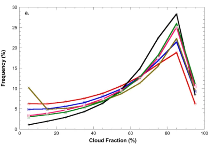
The net result of these observational biases is an increased correlation between AOT and COT, leading to an overestima-tion of AIE through either anomalously high AOT retrievals and/or the impacts of upstream atmospheric conditions. In an ideal scenario, the uncertainty in AOT could be reduced by removing MODIS pixels with a cloud fraction greater than some value. However, by doing this, we remove data asso-ciated with some of the highest aerosol concentrations and thickest clouds, where AIE are most likely to be observed. For all regions, well over 50% of the data correspond to cloud fractions of 50% or greater (Fig. 2a). Removing these data would introduce an unacceptable sampling bias to the results. Instead, we use all available AOT data and note that uncer-tainties due to clouds may account for some portion of the correlation in aerosol and cloud properties.
Bulgin et al. (2008) makes the assumption that aerosol ob-servations in the vicinity of clouds are adequate in lieu of co-incident observations when averaged over large spatial (1◦) and temporal (seasonal) scales. Despite this assumption not being completely accurate, the resulting overestimation of AIE was deemed small. Since truly independent measure-ments of aerosol and cloud properties using satellite-based methods are not practical, we too make the same assumption and note the resulting uncertainty it introduces. Further ev-idence for the validity of this assumption was presented by Andreae (2009). To assess the impacts of near cloud biases in AOT and FMF in this research, both values are analyzed as a function of MODIS cloud fraction for each region. For cloud fractions greater than 60%, a positive relationship ex-ists between cloud fraction and AOT for all regions except BB (Fig. 2b). The average increase in AOT between cloud fractions of 60% and 100% is approximately 0.1 over the AOT when cloud fraction is less than 60%. Interestingly, this increase is about the same irrespective of the AOT values at low cloud fractions.
Several factors may be responsible for the increase in AOT. First, larger concentrations of aerosols may be indeed present near clouds, which would be consistent with indirect the-ory. However, it may also be possible that AOT is higher because of the increase in size of humidified aerosols near clouds as discussed previously. It is likely both are simulta-neously being observed here. To determine what impact the change in aerosol size is having, MODIS FMF is also plot-ted against cloud fraction (Fig. 2c). For all regions except IO and EA, a small decrease in FMF occurs as cloud frac-tion increases. The lower FMF values are evidence for the larger humidified aerosols expected in the vicinity of clouds. However, the change in FMF from 0 to 100% cloud frac-tion is less than 15% (except for IO, where FMF increases as a function of cloud fraction). In the eastern North Atlantic mineral dust represents the primary aerosol type, which is
Fig. 2.Frequency(a), aerosol optical thickness(b), and fine mode fraction(c), binned as a function of MODIS cloud fraction for each region of study. Note that the maximum number of pixels occur when cloud fraction is approximately 80%. AOT increases as a function of cloud fraction due to both hygroscopic aerosol growth and indirect effects. FMF decreases approximately 15% for all re-gions except EA, where change is minimal, and IO where an in-crease is present.
generally non-hygroscopic. As a result, FMF would not be expected to decrease as a function of cloud fraction, at in fact remains nearly constant. The increase in FMF relative to cloud fraction in IO occurs as a result of small concentrations of fine mode aerosols (either anthropogenic or DMS) being present on top of the natural sea-salt background and/or pos-sible nucleation of sulfate particles through aqueous chem-istry. Since AOT is higher in these circumstances, AIEs and increased cloud cover is more likely. For the other regions, the differences in FMF are generally less than the relative change in AOT as a function of cloud fraction indicating that at least a portion of these changes is due to other fac-tors beside humidified aerosol growth. Thus, when changes in aerosol and cloud properties exceed 15%, then it is likely either AIE and/or atmospheric conditions are affecting the interaction between aerosol and cloud properties.
atmospheric conditions. Positive AI values indicate the pres-ence of UV-absorbing aerosols in the mid and upper tropo-sphere, while near zero and negative values are indicative of non-absorbing, scattering, and/or, fine-mode aerosols near the surface.
For comparison purposes, data from the CALIOP instru-ment on the CALIPSO satellite are obtained for the 2006– 2007 time frame, and seasonal averages of aerosol height for each region calculated. The CALIOP is an active lidar that provides vertical profiles of backscatter at 532 and 1064 nm that sample the vertical distribution of clouds and aerosols in the atmosphere (Vaughan et al., 2004). We use aerosol-layer height retrievals from the CALISPO Level 2 ALAY5-V2 product, which is still in its preliminary stages of valida-tion. While uncertainties are high, these data do provide a quantitative assessment of aerosol height not available from the other instruments and are especially useful at examin-ing differences in aerosol heights from region to region. We use the maximum aerosol layer height for our calculations; thus, resulting layer averages represent the maximum height to which aerosol are transported within any particular region. Thus, aerosols may (and likely do) exist below this layer as well. Since the dates of CALIPSO data availability do not overlap with the primary dataset used in this study, we as-sume that the 2006–2007 seasonal averages of AOT height for each region are consistent with previous years. The sum-mer season consists of June, July, and August data (JJA) from 2006 and the winter season consists of data from December, January, and February (DJF) during 2006–2007.
2.3 Meteorology
Daily, global surface wind speed and direction, and relative humidity at 1000, 850, and 700 hPa levels are obtained from National Center for Environmental Prediction (NCEP) Re-analysis data. The NCEP ReRe-analysis contains global me-teorological conditions with a 2.5 degree horizontal resolu-tion and a 17 level vertical resoluresolu-tion (1000–10 hPa) at 6 h time intervals (00:00, 06:00, 12:00, 18:00 UTC) (Kalnay et al., 1996). The reanalysis data set reliability captures synop-tic scale dynamic and thermodynamic features, though often misses smaller scale phenomena. While all these parame-ters are compared to indirect effects to some extent, vertical velocity in particular is used to determine whether or not a certain region is favorable or unfavorable for cloud forma-tion. NCEP data nearest in time to the satellite overpass time in each region are used. For example, if the overpass time is 14:00 UTC, satellite data are combined with NCEP data at 12:00 UTC.
3 Methodology for calculating AIE
All statistics such as correlations and regression coefficients between aerosol and cloud properties are computed using
the CERES pixel-level data (with a daily temporal resolu-tion and a∼20 km spatial resolution) within each 10×10◦ region for each month of data. Pixel-level data for each one-month period are averaged to form one-monthly averaged values from which time-series of aerosol, cloud and atmospheric conditions are constructed. Anthropogenic and dust direct and indirect radiative effects are calculated using a modified form of the methods outlined by Quaas et al. (2008). As part of this process, the total AOT (τ) must be separated into its maritime (sea-salt), dust, and fine-mode constituents. For the purposes of this research, fine-mode aerosols are considered to be primarily anthropogenic in origin and are labeled as such. The Kaufman et al. (2005b, c) method is employed to calculate the portion of AOT resulting from each aerosol type (Jones and Christopher, 2007). This method assumes that maritime AOT is primarily a linear function of near surface wind-speed and that maritime (τma), dust (τdu), and
anthro-pogenic (τan) aerosols each have characteristic FMF values
that can be used as separation points between each aerosol type. The characteristic FMF values used here are the same as those employed by Jones and Christopher (2007), which do not vary as a function of region, but are allowed to vary as a function of time. The dust and anthropogenic components of AOT are derived by solving a series of mathematical rela-tionships where maritime AOT is known, and one remaining unknown,τduin this case, removed from the series of equa-tions. The remaining component (τdu)is simply defined by subtracting τan andτma from observed AOT. Uncertainties in this method are explained in detail in Jones and Christo-pher (2007, 2008), where it is noted that the component AOT values have an uncertainty of between 30 and 50%. Quaas et al. (2008) used the method outlined by Bellouin et al. (2005) to calculate the anthropogenic portion of the AOT. However, this method does not discriminate between sea-salt and dust aerosols, preventing the calculation of dust-only direct and indirect effects.
Dust direct radiative effect (DRE) and Direct Climate Forcing (DCF) due to anthropogenic aerosols are calculated using the incoming solar radiation derived from the satel-lite overpass time, solar zenith angle, and earth-sun distance, and then applying a diurnal adjustment factor (D) (Bellouin et al., 2005; Jones and Christopher, 2007). Unlike Quaas et al. (2008), we apply the diurnal adjustment method used by Remer and Kaufman (2006) and the differences between these adjustments are small. The diurnally averaged DCF due to anthropogenic aerosols (1Fa) can be expressed as
the change in planetary albedo due to anthropogenic aerosols (1αa)multiplied by the incoming solar radiation at the top
of the atmosphere (Fs)as shown in Eq. (2).
1Fa=1αaFs (2)
The change in planetary albedo due to anthropogenic aerosols is expressed by Eq. (3).
1αa = dα
Combining Eqs. (2) and (3) and using the empirical relation-ship derived for dα/dln(τ), the anthropogenic DCF becomes
1Fa= −(1−f )a2[ln(τ )−ln(τ−τan)]FsD (4) wherea2is a constant defined by Quaas et al. (2008) andf is the total cloud fraction. These and the following constants are computed as a function of season over several ocean do-mains and the appropriate values for each region are used. To calculate dust DRE (1Fd), the term ln(τ−τan)is simply
replaced by ln(τ −τdu)forming Eq. (5).
1Fd = −(1−f )a2[ln(τ )−ln(τ −τdu)]FsD (5)
This research does not compute DRE using CERES short-wave radiance observations like previous research that use CERES-SSF data (e.g. Jones and Christopher, 2007). The primary reason is that we want to compare direct and indirect effects of aerosols in the same region, and using compatible methods greatly simplifies this process. Also, the method used here already takes into account the effect of cloud-cover eliminating the need for any sort of bias adjustment (Christo-pher and Jones, 2008).
The cloud albedo effect (or first indirect effect) is a func-tion of the relafunc-tionship between the number density of liquid water droplets in a cloud (Nd) and the AOT. Number density
is not reported directly within the CERES-SSF product and must be calculated using cloud optical thickness (τc)and ef-fective droplet radius (re). Assuming adiabatic conditions, Brenguier et al. (2000) derive this relationship to be
Nd=γ τc1/2re−5/2 (6)
whereγ=1.37×10⁻⁵m−0.5. The first anthropogenic indirect effect (1Fia1)can be expressed by Eq. (7), where A(f,τc)is
empirical function relating albedo to cloud fraction and cloud optical thickness. This function is explained in detail in the Appendix of Quaas et al. (2008).
1Fia1= −f A(f, τc)
1 3
dln(Nd)
dln(τ ) [ln(τ )−ln(τ−τan)]FsD (7) When the correlation between N andτ is positive (e.g. more aerosols=more cloud droplets), the indirect effect becomes negative, cooling the atmosphere. If the correlation is nega-tive, then1Fia1becomes positive, opposite to the expected first indirect effect. To calculate the dust aerosol indirect ef-fect (1Fid1), the same substitution that is made for the direct effect (Eq. 4) is made to Eq. (7). The termdln(Nd)/dln(τ )
represents the linear regression fit between the natural loga-rithm of cloud droplet number density and AOT. This value is calculated on a month-by-month basis and is unique to each region studied. Uncertainties in this relationship are the greatest contributor to uncertainty in the reported in indirect effects using this method (Andreae, 2009).
Some clues about the second indirect effect, or cloud life-time effect, were also described by Quaas et al. (2008). How-ever, given the large uncertainties present in the relationship
between cloud fraction, cloud liquid water path (LWP), and going from number density to AOT, we chose to primarily focus our results on the first AIE. The term “aerosol indirect effect” in the following discussion refers to the first AIE com-ponent only unless otherwise stated. We fully recognize that several uncertainties in both observations and cloud-aerosol interactions exist that complicate the interpretation of the re-sulting AIE values (in addition to the cloud contamination described above). Uncertainties in the aerosol classification process, which are described above, also result in an addi-tional uncertainty for the dust vs. anthropogenic radiative ef-fects. Based on known uncertainties, a 30% difference be-tween dust and anthropogenic effects must exist for it to be considered significant.
4 Results
4.1 Regional direct and indirect effects
A suite of general circulation models estimate that anthro-pogenic indirect effects range from −1.9 to −0.3 Wm−2 globally (Lohmann and Feichter, 2005; Forster et al., 2007). More recent observational studies indicate that the total an-thropogenic AIE is likely on the lower side of this range, and possibly negligible in certain regions (Matsui et al., 2006; Quaas et al., 2008). No corresponding statistics for the indi-rect effects of dust aerosols are known to the authors. This research does not report globally averaged values, but instead focuses on regional differences in both the dust and anthro-pogenic indirect effects to determine under what conditions these effects are most likely to occur (Fig. 1). Table 1a,b lists dust and anthropogenic direct and indirect effects de-rived using the methods descried in Sect. 3 compared with cloud and aerosol properties derived from MODIS. Direct and indirect radiative effects reported here are diurnally aver-aged with no clear-sky bias adjustments necessary (Christo-pher and Jones, 2007; Quaas et al., 2008). AIE values are only reported where a statistically significant relationship be-tween AOT andRcexists for a particular one-month period. Recall that Eq. (7) is highly dependent on the relationship between AOT and N, where N is also a function ofRc. If this relationship is not significant, then any AIE values cal-culated using this equation would naturally be suspect. For the purposes of this work, statistically significant is defined as a 99% or greater confidence level using paired Student’s T test. (Effective sample size is used to compute these statistics and represents approximately 50% of the original sample size due to auto and spatial correlation of the raw data). While the correlation between AOT andRc is expected to be negative
when AIE is present, statistically significant positive correla-tions are not removed; thus, AIE “warming” is allowed to be included in the averages listed in Table 1b.
Table 1.Six year mean aerosol and cloud properties, and direct radiative effects for each region of study(a)Average dust and anthropogenic AIE for each region, with corresponding standard error values(b)Seasonally averaged of CTP (hPa) and total AIE (Wm−2) with seasonal averages (DJF and JJA, 2006–2007 only) of CALIPSO aerosol layer height (km), a.s.l. also listed.
a
Region Code AOT τan τdu DREan DREdu COT CF Rc CTP
[Wm−2] [Wm−2] [%] [µm] [hPa] Arabian Sea AS 0.33 0.16 0.11 −3.0 −1.0 1.9 57.8 14.2 852 Bay of Bengal BB 0.27 0.16 0.05 −3.2 −0.4 2.0 63.9 15.1 824 S. Indian Ocean IO 0.13 0.04 0.02 −0.9 −0.3 3.0 68.8 16.1 838 East North Atlantic EA 0.39 0.13 0.20 −1.4 −1.6 2.1 58.3 14.2 844 West North Atlantic WA 0.20 0.11 0.03 −3.3 −0.3 3.9 63.7 12.5 830 African Biomass AF 0.32 0.22 0.05 −2.8 −0.4 3.3 66.0 11.8 853
b
Region AIE DJF JJA
DUST ANTH H CTP AIE H CTP AIE
[Wm−2] [Wm−2] [km] [hPa] [Wm−2] [km] [hPa] [Wm−2] AS −0.18±04 −0.09±03 1.5 864 +0.10 3.3 801 −0.78 BB −0.01±.02 +0.01±0.04 1.4 833 +0.06 2.5 755 +0.22 IO −0.30±02 −0.43±03 1.1 823 −0.54 1.2 829 −0.64 EA +0.07±04 +0.05±03 1.9 812 +0.33 3.3 830 −0.43 WA −0.11±01 −0.46±06 1.3 819 −0.48 1.4 805 −0.89 AF −0.03±02 −0.31±12 2.8 812 −0.01 3.1 871 −0.45
average of total column AOT is greater than 0.25 for re-gions AS, BB, EA, and AF. The combined dust and anthro-pogenic direct effects range between−3.0 and−4.0 Wm−2. However, corresponding AIEs do not necessary correspond to higher AOTs. The two regions with the lowest AOT: WA and IO, (τ=0.20, 0.11, respectively) both produce the two largest values for total AIE (−0.57,−0.73 Wm−2). In IO, the total (anthropogenic + dust) indirect effect of−0.73 Wm−2 is not that much less than the corresponding DRE value (−1.2 Wm−2). Most of the AIE is from the anthropogenic component despite the lack of any nearby source of anthro-pogenic aerosols. However, approximately 50% of the total AOT is comprised of sea salt aerosols that are not accounted for in the direct and indirect calculations presented here and it is also possible fine mode aerosols such as DMS are be-ing falsely classified as anthropogenic. While total AOT is also low in WA, fine mode primarily anthropogenic aerosols account for over 50% of the total AOT.
In regions where AOT is greater than 0.25, AIEs are observed under certain circumstances, but not others. In AS, a total AIE is−0.27 Wm−2, with over 60% being ac-counted for by the dust component, which may have a hy-groscopic coating (Satheesh et al., 2006). If this is the case, then the largest AIE values would be expected when dust AOT is greatest so long as a significant anthropogenic aerosol background remains. In AF, average AOT is 0.32,
but the dust + anthropogenic direct radiative effect is only
−3.1 Wm−2, somewhat less that expected for this aerosol concentration. However, this region contains the largest pro-portion of black carbon aerosols, which also absorb solar radiation and warm the atmosphere, which in turn reduces shortwave radiative efficiency while increasing atmospheric stability (Matsui et al., 2006). Here the anthropogenic AIE is
−0.31 Wm−2with the dust effect being only−0.03 Wm−2. For BB and EA, both the dust and anthropogenic AIEs are small, indicating that other factors besides aerosols are significantly contributing to droplet growth, or lack thereof. In EA, the primary aerosol species is dust, which has usu-ally not been thought of as good CCN (Levin et al., 1996). Unlike in AS, no significant concentration of anthropogenic aerosols exists to coat the dust and increase their solubility. BB is more of a mystery since sulfates account for a large proportion of the total AOT, with anthropogenic AOT and cloud property retrievals all being similar to those observed in AS. One key difference is that the concentration of ele-vated dust aerosols is much less in BB compared to AS (Ta-ble 1a, b). The physical mechanisms behind the differences in AIE from region to region are examined in detail in the following section.
Table 2. Total AIE binned by thin (LWP<20 gm−2)vs. thick (LWP≥20 gm−2)clouds and 850 hPa upward (ω<0 Pa s−1)vs. downward (ω>Pa s−1) vertical motion(a). Percentage of months (out of a possible 70) that a statistically significant relationships exists between AOT andRc(b). Sample size of each bin in terms of percent of total sample size(c). Percentage difference between the regression fit between
AOT andRcover the range of AOT where the relationship is significant(d).
a
Region (LWP<20,ω>0) (LWP<20,ω<0) (LWP>20,ω>0) (LWP>20,ω <0) AS −0.17±.03 −0.17±.03 −0.34±.05 −0.59±.07 BB −0.04±.03 −0.01±.04 +0.01±.10 −0.02±.04 IO −0.43±.02 −0.53±.02 −0.74±.03 −0.85±.03 EA +0.11±.04 +0.101±.05 +0.13±.08 +0.32±.10 WA −0.29±.03 −0.24±.05 −0.84±.11 −0.91+10 AF −0.19±.10 −0.24±.10 −0.45±.14 −0.49±18
b
AS 81 71 70 50
BB 60 50 43 51
IO 74 66 100 100
EA 81 70 70 71
WA 57 33 57 61
AF 59 46 77 60
c
AS 60 19 8 13
BB 51 20 15 14
IO 12 8 44 36
EA 42 27 17 13
WA 29 13 29 30
AF 33 15 36 17
d
AS 39 41 44 46
BB 28 37 31 23
IO 31 31 21 21
EA 31 33 33 28
WA 24 33 33 28
AF 22 29 28 28
overall AOT and AIE (Jones and Christopher, 2008; Yuan et al., 2008). To assess the relative importance of aerosol concentrations and atmospheric conditions to cloud proper-ties, AIE is examined as a function of thin (LWP<20 gm−2)
vs. thick (LWP≥20 gm−2) clouds and whether or not corresponding 850 hPa vertical motion is upward or down-ward (approximately representing conditions favorable and unfavorable for cloud formation and persistence). Recall that previous research has shown that AIE are more likely to oc-cur in thicker clouds, often defined using LWP thresholds between 20 and 100 gm−2to separate thick from thin clouds (e.g. Lohmann et al., 2000; Lee et al., 2009). Similarly, thicker clouds should occur more often in the presence of up-ward motion; thus, AIEs should be greatest when both condi-tions are met. Table 2a lists total (anthropogenic + dust) AIE for each region averaged over a six-year period for months where a statistically significant relationship exists between AOT and Rc. The percentage of months where this
rela-tionship is significant is also listed (Table 2b), with 100% indicating a statistically significant relationship exists for all 70 months of data analyzed. It should be noted that given the differences in samples sizes and distributions between each bin, an average of the four AIE values may not correspond exactly to the average (listed in Table 1b) calculated using the entire data set for a particular region.
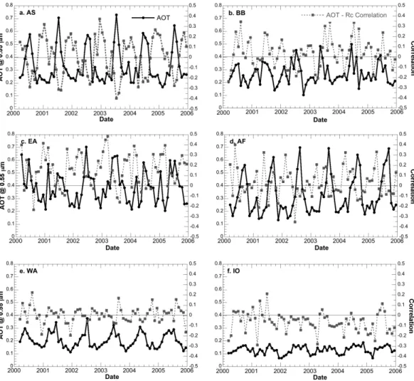
Fig. 3.Monthly mean MODIS total column AOT and correlation between AOT andRcfor each region between 2000 and 2006. Correlations
in excess of±0.1 are generally considered statistically significant. The time series of AOT –Rccorrelation is the gray line, and set to the
right hand axis on each plot.
samples being 4×and 2×that of the thin cloud samples. For these two regions, the difference between thick clouds asso-ciated with upward motion vs. downward motion is generally smaller, being only 10–15%. IO has the largest AIE values of the six regions studied, with thick maritime stratus clouds accounting for 80% of the sample. As before, AIE is great-est where thick clouds and upward motion are present. The difference in AIEs is generally greater between thick clouds vs. thin clouds compared to rising vs. sinking motion, but upward motion combined with thicker clouds did increase AIE compared to thick clouds associated with downward (or little) vertical motion for each of these four regions provid-ing evidence that atmospheric conditions must be considered when estimating AIE. In fact, part of this increase may be due to adiabatic cooling associated with rising parcels of air in al-ready humid environments. This cooling increases RH, fur-ther promoting the formation of clouds, while also increas-ing the possibility of humidified aerosols as well. For most regions, relative humidity was indeed greatest for the thick
cloud, upward motion sample. However, when comparing AIE against solely RH, no significant relationships could be found. If adiabatic cooling was the dominant source for AIE, then the relationship between AIE and RH should be more apparent; thus, we do not believe that the increase in AIE for this sample is primarily due to this effect. While the 6-year averages indicate that AIE are indeed greatest for thick clouds in the presence of upward motion in regions AS, IO, WA, and AF, indirect effects also existed for the other cases. What this means is that indirect effects can still occur un-der less than ideal conditions, but that the magnitude of the effects will generally be less.
Regions BB and EA appear to behave differently than the four regions described above.
Fig. 4.Monthly averaged NCEP 850 and 700 hPa relative humidity (%), 850 hPa vertical velocity (Pa s−1), and MODIS cloud fraction for each region. Upward motion is indicated by negative values.
humidity, and relative positions of the cloud and aerosols layers. These possibilities are explored in detail below in the following section. In EA, AIE values are weakly positive in all cases, opposite that expected. Even more interesting is that the warming is greatest for thick clouds associated with rising motion (+0.32 Wm−2). In EA, it has been sur-mised that the semi-direct effect (warming from absorbing aerosols), outweighs the importance of the microphysical aerosol – cloud relationship normally expected for AIEs. This warming can lead to subsidence and/or increased cloud evaporation, reducing cloud cover and possibly AIE.
To determine if the estimates of AIE are indeed significant and not just a result uncertainties AOT retrievals near clouds, we use the magnitude of the change in effective cloud ra-dius as a function of AOT as a guide. For each of the four cloud-type, vertical motion samples created above, if the lin-ear regression fit between AOT andRcis statistically
signif-icant (and negative), and the fittedRcvaries more than 15%
between the minimum and maximum observed AOT, then at least a portion of the relative changes between aerosol and
cloud properties is deemed to be a result of aerosols, and not artifacts. This difference threshold is based on the difference in FMF observed as a function of cloud fraction for each re-gion shown in Fig. 2c and discussed in Sect. 3. The largest differences (∼40%) occur in AS, and are maximized for the upward motion, thick cloud sample; thus, we are quite confi-dent that the results from this region are not due to observa-tional artifacts. Most other regions and samples have differ-ences of∼30%, which also exceeds our predefined thresh-old by a factor of 2. While the differences in AOT andRc
are considered physically meaningful using the tests applied here, they do not necessarily indicate that large AIE are oc-curring.
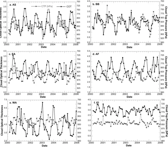
Fig. 5.Monthly averaged cloud optical thickness (COT) and cloud top pressure (CTP, hPa) for each region.
be considered significant. In IO, FMF actually increases with cloud fraction, completely opposite that expected by the FMF test. However, the aerosol – cloud interactions in these two regions are substantially different from those in the other four regions and the details of which are described below. 4.2 Seasonal variation in AIE
4.2.1 Arabian Sea (AS)
Aerosol indirect effects vary substantially as a function of time in all regions; thus, it is important to analyze aerosol, cloud, and atmospheric conditions as a function of time to assess the specific physical processes occurring. In the AS, the maxima in cloud fraction and COT during JJA correspond well with maxima in 850, 700 hPa humidity and 850 hPa ver-tical velocity (Figs. 3–6a). In fact, most of the thick-cloud, upward motion sample shown in Table 2a occurs during JJA, with very few points present outside the summer months. AOT is also maximized at the same time, primarily from an influx of elevated dust aerosols and increased production of sea salt due to higher wind speeds. Correlation betweenRc
and AOT is indeed most negative in JJA with a correlation coefficient of−0.3 averaged over JJA for all years. Similar results were observed by Patra et al. (2007), also indicating maximum indirect effects during the summer months. The cloud droplet effective radius is also greatest during the sum-mer months, when moisture and cloud thicknesses are great-est. This differs from the finding by Chylek et al. (2006) who observed smaller droplet radii in September (high AOT) compared to larger radii in January (low AOT). However, their spatial domain was substantially larger than used here; thus, their statistics are not necessary valid for the smaller Arabian Sea domain used by this research.
Both anthropogenic and dust AIEs are maximized in the summer, with values near −1.0 Wm−2, consistent with ex-pectations (Fig. 6a). Based on the magnitude of the change in
Rcrelative to AOT (>40%), these estimates of AIE are
con-sidered a reflection of process outlined by Twomey (1977) and many others. The difference in AIE values between sum-mer and winter estimates is also significant. In the winter, the correlation between Rc and AOT is weak resulting in
Fig. 6. Monthly averaged direct and indirect dust (DU) and anthropogenic (AN) aerosol effects. Note the seasonal variability of direct radiative effects in all regions, which is consistent with the seasonal variability of total AOT in Fig. 3. Indirect effects only show seasonal cycles for certain regions, and are generally smaller that direct radiative effects.
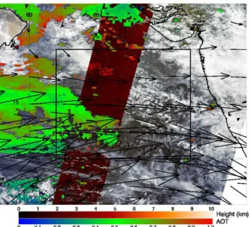
Fig. 8. Terra MODIS three band overlay for 8 August 2003 with AOT at 0.55µm from both MODIS and MISR overlaid. The MISR stereo height product represents the height above sea level the upper most cloud layer is located. Vectors indicate 850 hPa wind speed and direction.
monthly averagedRcalso being small compared to the
over-all mean value (11.0 vs. 14.2µm). Here, atmospheric hu-midity is less and vertical motion is weak, inhibiting cloud formation leaving relatively thin clouds as evidenced by the decrease in COT (Figs. 5a, 7a). Comparison of thin (LWP<20 gm−2)vs. thick (LWP>20 gm−2)clouds shows that total AIE associated with the thick cloud sample is nearly double that associated with the thin cloud sample (Table 2a). While total AOT is greatest during the summer months, an-thropogenic DRE is maximized during November and De-cember when the anthropogenic portion of the AOT is great-est with values exceeding−5.0 Wm−2(Fig. 6a).
The question remains as to whether or not the dust AIE reported here is actually from pure dust aerosols only. It is possible that that some maritime sea salt aerosols are being classified as dust by the algorithm. Dust coated with sul-fates may also be part of the dust component (Levin et al., 1996; Seinfeld and Pandis, 1998); thus, causing “dust” AIE to appear larger than AIE from the fine mode component of aerosol alone. Between June and August (JJA), sustained upward vertical motion from near the surface up to at least 600 hPa may be aiding both by transporting anthropogenic aerosols high enough into the atmosphere to interact with some of the dust aerosols present (Fig. 7b). Since AIE val-ues for both dust and anthropogenic aerosols are similar and given the uncertainties inherent in the aerosol classification process, we cannot unambiguously determine which is most important in this region. However, the results strongly in-dicate that both aerosol types, possibility mixing with each other, are important to AIE in this region.
Fig. 9.Frequency histograms of MISR stereo height (km) for each selected example. All regions except BB have a large peak below 3 km, whereas BB indicates a greater proportion of clouds above 10 km.
Finally, it is important to determine whether or not the el-evated dust aerosols are co-located with cloud heights. To examine this last question, we compare the seasonally av-eraged cloud top pressures derived above with CALIPSO aerosol layer heights for winter (DJF) and summer (JJA) time periods. In this region, aerosol layer height increases from 1.6 km in DJF to 3.3 km in JJA, primarily corresponding to the influx of dust aerosols (Table 1b). For the same time periods, CTP is 864 and 805 hPa or approximately 1.3 and 2.1 km above the ocean surface. These layers are somewhat below the maximum aerosol height layers from CALIPSO; however, the aerosol layer averages only represent a maxi-mum ceiling to the aerosols. As such, they are also likely to exist below this height as well. Since these thicker clouds occur within a deep layer of aerosols, some of which are hygroscopic by nature or coating, AIE should be most sig-nificant during this period and the seasonally averaged total AIE agrees with this hypothesis (+0.10 vs.−0.78 Wm−2, Ta-ble 1b).
Fig. 10.Same as Fig. 7, but vertical velocities corresponding to date and time of the MODIS-MISR examples for regions AS, BB, EA, and AF ,respectively. Note that upward motion below the freezing level is generally greatest in AS.
which is−0.35. Overall, comparisons of aerosol and cloud properties within this region support the hypothesis the AIE is more likely to occur where upward vertical motion and thicker clouds are present.
4.2.2 Bay of Bengal (BB)
In the Bay of Bengal, a similar pattern exists as in the Arabian Sea. AOT is maximized in the summer due to increase dust aerosol transport and some increase in sea-salt production. The magnitude of this increase is much smaller than that ob-served in AS (τdu=0.05 vs. 0.11), and fine mode aerosols
ac-count for larger proportion of the total AOT. Comparisons of model and observed aerosol speciation by Jones and Christo-pher (2007) suggest that the fine mode aerosols consist pri-marily of sulfates. The mean anthropogenic AOT component is nearly identical for both regions (τan=0.16). As in the Ara-bian Sea, anthropogenic DRE is maximized during the winter with values between−6 and−8 Wm−2(Fig. 6b). The corre-sponding increase in summertime dust DRE is much smaller (−1.0 Wm−2). Cloud fraction, cloud droplet effective radius, AOT, relative humidity, and upward vertical velocity are all again maximized in the summer. Unlike the Arabian Sea, no corresponding increase in the either anthropogenic or dust AIE is readily apparent (Figs. 3b, 6b). Binning data relative to thick vs. thin clouds, or upward vs. downward 850 hPa ver-tical motion did not produce a sample where significant AIE is present (Table 2a).
Fig. 11. Terra MODIS three band overlay for the Bay of Bengal on 23 July 2003, but otherwise similar to Fig. 8. Note the greater amounts of cirrus compared to low level stratus in this example compared to other regions.
between cloud and aerosol layer properties, limiting AIE (Ta-ble 1b). If the clouds were thicker (i.e. extending from near the surface to the 800 hPa layer), COT should be higher than observed in AS. This is not the case as both had averaged values of near 2 (Table 1a); thus, cloud bases in BB must also be higher. Unfortunately given the data available, we cannot further quantify the relative importance of these dif-ferences, but only state that these represent possible reasons that are consistent with expectations and previous research.
However, we can analyze the situation in more detail through a case study. In the Bay of Bengal, at least two cloud layers are present in an example from 23 July 2003 (Fig. 11). The most predominate cloud type appears to be cirrus clouds resulting from small pockets of convective ac-tivity with heights above 10 km a.s.l. Below this layer exist a few maritime status and cumulus clouds, but their over-all areal coverage is low. The distribution of MISR stereo heights within this region exhibits a distinct bi-model distri-bution, with maxima at 2 and 10–11 km (Fig. 9). NCEP data at 15◦N and 90◦W also shows a bi-modal distribution of ver-tical velocity with two levels where upward motion is maxi-mized, 850 and 300 hPa (Fig. 10). Relative humidity is also high (86%) at this level indicating the presence of this second cloud layer. Mean TOMS-AI is much lower (0.4) than in the Arabian Sea, which is due to a lower elevated dust aerosol concentration. As previously noted, aerosols in the Bay of Bengal are generally anthropogenic in nature with the great-est concentration likely present with the maritime boundary later (<1.5 km). Most of the clouds in this example appear to be located above the aerosol layer limiting the probably, or at a minimum, the observability of the indirect effect on liquid water clouds. These observations are consistent with the long term time-series analyzed above, and provide fur-ther evidence that cloud formation at least in this case is less favored in the Bay of Bengal.
4.2.3 Eastern North Atlantic (EA)
In the eastern North Atlantic, aerosols primarily originate from dust over the Saharan Desert and are advected westward by the prevailing winds (Dunion and Veldon, 2004; Kaufman et al., 2005b). Elevated dust aerosol concentration is maxi-mized in the late spring and summer months, leading to a sea-sonal cycle in AOT and dust DRE (Figs. 3–6c). CALIPSO data for JJA 2006 indicated that these aerosols are located be-tween 3 and 4 km above the ocean surface (Table 1b). Cloud fraction remains approximately constant at 60% with the ex-ception of decreases occurring during the months of Decem-ber and January (Fig. 4c). While cloud fraction does not change substantially, COT does increase during the summer months in association with the northward movement of the ITCZ. During this time, atmospheric moisture is maximized and overall vertical velocities are near zero. (Upward vertical motion is present within the individual convective elements along the ITCZ, but the poor resolution of the NCEP data
washes out much of smaller scale upward motion actually present.) By contrast, very low humidity (<30%) exists dur-ing the winter months when strong subsidence also present.
There does exist a seasonal cycle in the relationship be-tween AOT andRc, with a statistically significant positive
correlation present during the winter months, where AOT and moisture content are lower (Fig. 5c). In the summer the correlation is often near zero. This cycle is consistent with that observed in the Arabian Sea, with the exception that the AOT –Rc correlation never quite becomes
consis-tently negative. The overall dust and anthropogenic AIEs are small (+0.03 and +0.05 Wm−2)and mostly positive, in-dicating a slight warming effect. Interestingly, AIE is most positive for the thick-cloud, upward motion sample with a value of +0.32 Wm−2even though it is here where the great-est cooling would generally be expected (Table 2a). Neg-ative AIE values due to dust and anthropogenic aerosols are only observed in JJA, and the average JJA value re-ported (−0.43 Wm−2)is skewed negative somewhat by three months where total AIE exceeds−1.0 Wm−2.
Table 3. MODIS AOT and CTP, TOMS-AI, MISR Stereo heights, NCEP vertical velocity at 850 hPa (Pa s−1), and derived dust and anthropogenic AIE (Wm−2) for the days corresponding to the examples shown in Figs. 7, 9–11.
Region Date AOT AI CTP MISR ω850 IEdu IEan
[hPa] [km] [Pa s−1] [Wm−2] [Wm−2] AS 8 Aug 2003 0.58 1.8 800 3.6 −0.18 −2.1 −0.1 BB 23 Jul 2003 0.22 0.4 721 10.7 −0.13 0.9 0.4 EA 23 Jul 2004 0.59 1.8 816 3.9 −0.06 −0.4 −0.4 AF 30 Sept 2004 0.61 1.5 860 1.5 0 0 −3.3
MODIS/MISR observations on 23 July 2004 show large dust aerosol concentrations west of the African coast (Fig. 12). Convective clouds extending up to 10 km a.s.l. ac-cording to MISR stereo height retrievals are present south of an 850 hPa low pressure center (−25◦W, 14◦N). However, the average cloud top pressure for liquid water clouds during this month is 842 hPa. Dust aerosols that may be above the freezing level (∼550 hPa) may act also as ice condensation nuclei (DeMott et al., 2003). This effect, however, is outside the scope of this research. Significant dust aerosol concen-trations are present with total AOT being 0.59 with a cor-responding TOMS-AI of 1.8. However, total AIE is only
−0.8 Wm−2. As with the overall monthly mean, vertical mo-tion is weak during this day, with even some subsidence be-ing observed as low as 700 hPa. This example does at least contain weak upward motion and a weak AIE compared to the neither in the long term sample, but with an AOT of 0.59, much greater AIE values would be expected if more of the aerosols were hygroscopic and non-absorbing.
4.2.4 Eastern South Atlantic (AF)
In the eastern South Atlantic off the African coast, aerosols primarily originate from biomass burning producing of large amounts of carbon based aerosols, especially between Au-gust and October (e.g. Lindesay et al., 1996). These aerosols are transported westward from central and southern Africa, leading to high AOT values (>0.6) with a mean aerosol layer height of approximately 3 km throughout the year (Ta-ble 1b). These aerosols produce an anthropogenic DCF of
−8.0 Wm−2in August and/or September, which is very con-sistent year over year (Fig. 6d). A secondary maximum in dust aerosol concentration and DRE is present during Febru-ary and March, with maximum values of−2.0 Wm−2. With the exception of 2001, 850 hPa atmospheric humidity and vertical velocity (consistent subsidence at all levels) do not change substantially as a function of time with over 70% of the sample consisting conditions where subsistence is present (Table 2c). Anthropogenic AIE is only present during these months for all years except 2001 and is greatest in the pres-ence of the thicker clouds (−0.45 Wm−2)with the upward motion sample only being slightly greater than the downward
Fig. 12. Terra MODIS three band overlay for the North Eastern Atlantic (EA) region on 23 July 2004.
Fig. 13. Terra MODIS three band overlay for the South Eastern Atlantic off Africa on 30 September 2004. Note the thick low-level stratus field present over most of the study domain.
On 30 September 2004 MISR observed cloud-heights only up to 2 km, while biomass burning aerosols are likely present even higher in the atmosphere as the TOMS-AI value for this day is 1.5 (Fig. 13, Table 3). In this example a large stratus deck exists over most of the region with an average CTP of 860 hPa. For this day, the anthropogenic AIE is−3.3 Wm−2 though vertical motion is weak throughout the atmospheric column (Fig. 10). If these AIE values are a reflection of ac-tual microphysical interactions, then significant aerosol con-centrations should also be present near the surface. Experi-ments during the SAFARI campaign and CALIPSO satellite observations noted significant aerosol concentrations from biomass burning are frequently trapped in a stable layer at or above 3 km a.s.l., allowing for transport well into the central Atlantic while aerosols below the boundary layer tended not to travel as far (Garstang et al., 1996). However, the region of study is close enough to the source region that aerosols at both levels are present. Also, the presence of the low-level stratus deck throughout the last half of the year while also noting that aerosols are also present near this layer has been obesrved. Both this, and the case study example described above support the notion that AIE does occur in AF, but that the cloud layer is generally quite low to the surface and that primarily boundary layer aerosols are responsible. As a re-sult, vertical motion and other atmospheric conditions above this layer are not as important as in other regions.
4.2.5 Western North Atlantic (WA)
Another region consisting of aerosols produced from anthro-pogenic pollution sources is present off the eastern coast of the United States. In the western Atlantic, AOT and DCF
is maximized in JJA in association with seasonal variations in industrial pollution and atmospheric transport patterns. However, overall upward vertical motion in JJA is relatively weak and shows no low level maximum like the Arabian Sea (Fig. 7b). As a result, most aerosols are trapped in the bound-ary layer below l.5 km (Table 1b). The correlation between AOT andRcis low during the summer months, still AIE is
greatest in JJA with an average value of−0.89 Wm−2 com-pared to−0.48 Wm−2in DJF (Table 1b, Fig. 6e), with the majority of AIE being from the anthropogenic component. Cloud cover and cloud thickness on the other hand are max-imized during the winter months though CTP remains ap-proximately constant (Table 2b), in response to low-pressure systems that propagate through this region. Comparing the thick cloud vs. thin cloud sample shows that total AIE is three times larger in the thick cloud sample (Table 2a), with most of that sample originating from summer data. Even with the inherent uncertainties present using this method, AIE values derived here exceed those required to be considered physi-cally significant. In addition, a similar certainty exists for the difference in thin vs. thick clouds, though upward motion only appears to increase AIE in the thick cloud sample. Thus, for this region it appears that conditions favorable for thicker and more persistent clouds are indeed important to the mag-nitude of AIE, more so than just the aerosol concentration it-self, consistent with the observations by Bulgin et al. (2008). The concentration of dust aerosols within this region remains small compared to the anthropogenic component and as a re-sult, dust AIE remains small.
4.2.6 South Indian Ocean
In a more pristine environment such as in the Southern In-dian Ocean, little variability exists in the overall atmospheric conditions (Fig. 4f). Maximum relative humidity occurs be-tween 850 hPa and the surface and vertical velocities remain low (Fig. 7). Overall, cloud fraction and COT also do not vary by more than±10% and±0.7 respectively, indicating that the primary cloud mode is maritime stratus with nearly 80% of the clouds having a LWP>20 gm−2.