Multiuser MIMO system using block space time spreading and tensor modeling

Multiuser MIMO system using block space– time spreading and

tensor modeling

Andre´ L.F. de Almeida

a

_{, Ge´rard Favier}

a,

_{, Joa˜o C.M. Mota}

b a_{I3S Laboratory, University of Nice-Sophia Antipolis (UNSA), CNRS, France}

b_{Wireless Telecom Research Group, Federal University of Ceara´, Fortaleza, Brazil}

a r t i c l e

i n f o

Article history:

Received 4 May 2007 Received in revised form 12 March 2008 Accepted 26 March 2008 Available online 8 April 2008

Keywords:

Blind detection MIMO system Multiplexing Multiuser interference Space–time spreading Tensor modeling

a b s t r a c t

In this paper, we consider a point-to-multipoint downlink multiuser wireless communication system, where a multiple-antenna base station simultaneously transmits data to several users equipped with multiple receive antennas. The transmit antenna array is partitioned into transmission blocks, each one being associated with a given user. Space–time spreading is performed within each block using a transmit antenna subset. We formulate block space–time spreading using a tensor modeling. We show that the tensor-based block space–time spreading model has the distinguishing feature of modeling a multiuser space–time transmission with different spatial spreading factors (diversity gains) as well as different multiplexing factors (code rates) for the users. The space–time spreading structure is chosen to allow a deterministic multiuser interference (MUI) elimination by each user. A block-constrained tensor model is then presented for the received signal, which is characterized by fixed constraint matrices that reveal the overall space–time spreading pattern. At each receiver, blind joint channel and symbol recovery is performed using an alternating least squares algorithm. Simulation results illustrate the performance of the proposed transceiver model in terms of bit-error-rate, channel/symbol estimation accuracy and link-level throughput.

&2008 Elsevier B.V. All rights reserved.

1. Introduction

Multiple-input multiple-output (MIMO) wireless com-munication systems employing multiple antennas at both ends of the wireless link are considered as one of the key technologies to be deployed in current and upcoming wireless communications standards [1]. They capitalize on spatial multiplexing, which aims at attaining the high capacity of MIMO fading channels[2–5], or on space–time (ST) coding[6–8]or different combinations of both[9,10]. Several works have addressed the design of MIMO signaling techniques for multiuser (MU) multiple-access systems, especially in the downlink, by using ST spreading

in conjunction with Direct-Sequence Code Division Multi-ple Access (DS/CDMA) techniques (see e.g.[11–14]and the references therein). By exploiting excess bandwidth, these approaches are generally based on the combination of linear ST spreading codes and MU spatial multiplexing at the transmitter, and rely on linear MU detection at the receiver side to handle multiuser interference (MUI). Ng and Sousa [11] proposes a ST multiplexing model that allows several users to simultaneously access all the spatial channels, by using mutually-orthogonal spreading codes for the transmit antennas. This idea is pursued in

[12], by using different ST multiplexing matrices (i.e. different 2-D spreading codes) for each user. In[13], ST multiplexing and algebraic rotation are combined to yield full transmit diversity to each user. The receiver is based on linear MU detection followed by single-user sphere decoding. Doostnejad et al. [14] proposes a ST multi-plexing model for the downlink of a MU ST MIMO system Contents lists available atScienceDirect

journal homepage:www.elsevier.com/locate/sigpro

Signal Processing

0165-1684/$ - see front matter&2008 Elsevier B.V. All rights reserved. doi:10.1016/j.sigpro.2008.03.020

_{Corresponding author. Tel.: +33 492 942 736; fax: +33 492 942 896.}

E-mail addresses:lima@i3s.unice.fr (A.L.F. de Almeida),

along with a new spreading matrix structure. All these approaches assume that the channel is perfectly known at the transmitter (or it has been estimated using training sequences), and rely on the orthogonality properties of the spreading codes to handle MUI elimination at the receiver. They also focus on suboptimal receiver structures as an alternative to maximum likelihood (ML) detection.

The use of tensor modeling in wireless communica-tions started with the seminal paper[15], which shows that a mixture of DS/CDMA signals received by an antenna array can be formulated using the PARAFAC decomposi-tion [16]. The paper proposes a blind MU detection receiver that relies on the identifiability properties of this tensor decomposition. Following [15] and considering more general propagation scenarii [17–22] propose dif-ferent tensor modeling approaches for MU wireless communication systems. The use of tensor decomposi-tions in MIMO antenna systems has been addressed in

[19,23–25] by focusing on single-user transmissions. In

[19], a generalized tensor model for MIMO systems was proposed. However, this modeling approach only con-siders spatial multiplexing. The MIMO system model of

[23] considers spreading of each data stream in the temporal dimension only, i.e. across consecutive chips. There is no spreading across the transmit antennas. In

[24], we proposed a constrained tensor model for MIMO systems which allows spatial spreading of each data stream across both space (antennas) and time (symbols) dimensions.

In this work, we propose a new modeling approach for the downlink of a MU-MIMO wireless communication system. In our MU-MIMO framework, a multiple-antenna base station simultaneously transmits data toQusers. The transmit antennas are divided intoQ different transmis-sion blocks, each one being associated with a given user. ST spreading is performed within each block using a transmit antenna subset. The proposed block ST spreading approach has the distinguishing feature of modeling a MU ST transmission with different spatial spreading factors (diversity gains) as well as different multiplexing factors (code rates) for the users. We consider an orthogonal ST spreading structure that allows a deterministic MUI elimination by each user. The received signal is formu-lated as a block-constrained tensor model [22,26]. We provide a physical interpretation for the constrained structure of this model by showing that it is linked to the block ST spreading pattern at the transmitter. At each receiver, blind joint channel and symbol recovery is performed after a MUI elimination stage, by using the classical ALS algorithm[15].

The proposed block-constrained tensor-based MU-MIMO system can be viewed as a generalization of

[23,24]due to the fact that (i) it is designed to cope with MU MIMO transmission and (ii) it jointly performs ST spreading and MU spatial multiplexing. This MU-MIMO framework is close to those of [11,12,14], which use ST multiplexing codes for downlink MU-MIMO systems. Our block ST spreading structure acts as a tridimensional (3-D) spreading sequence.

The organization of the paper is as follows. Section 2 describes the system model and assumptions. In Section 3,

we formulate the proposed block ST spreading system using tensor modeling. Performance analysis is carried out in Section 4. Section 5 formulates the received signal using a block-constrained tensor model. A physical interpreta-tion for the constraint matrices of this tensor model is presented in Section 6. In Section 7, the receiver algorithm is described. Simulation results for performance evalua-tion are presented in Secevalua-tion 8, and the paper is concluded in Section 9.

2. System model and assumptions

Let us consider the downlink of a MIMO MU wireless communication system where a multiple-antenna base station simultaneously transmits data toQusers employ-ing multiple receive antennas. LetPdenote the temporal spreading factor of the system. The base station is equipped withMT transmit antennas, and theq-th user is equipped with MR receive antennas, q¼1;. . .;Q

(see Fig. 1). It is assumed that the base station has no knowledge of the downlink channels.1

The transmission is organized into time-slots of N symbol periods, each one being composed ofPchips. We assume that the wireless channel is characterized by scattering-rich propagation and is frequency-flat. The channel is also assumed to be constant during the time necessary to transmit a time-slot, but varies between two consecutive time-slots. For theq-th user, the discrete-time baseband version of the signal received at the mR-th receive antenna, associated with thep-th chip of then-th transmitted symbol, can be written as

xðqÞ

mRððn1ÞPþpÞ ¼

XMT

mT¼1

hðqÞ

mR;mTcmTððn1ÞPþpÞ,

n_¼1;. . .;N; p¼1;. . .;P,

wherehðqÞ

mR;mTis the complex channel gain between themT -th transmit and -themR-th receive antenna andcmTððn1Þ

PþpÞ is the ððn1ÞPþpÞ-th sample of the signal transmitted by the mT-th transmit antenna. Let HðqÞ 2

C

MRMT andCn2

C

MTPdenote the MIMO channel matrix

and the transmitted signal matrix at the n-th symbol period. LethðqÞ

mR;mT¼:½HðqÞmR;mTandcmTððn1ÞPþpÞ¼:½CnmT;p

be the typical elements of these matrices. Taking these definitions into account, we can represent the noiseless received signal at then-th symbol period by an MRP matrixXðqÞ

n , withxðmRqÞððn1ÞPþpÞ ¼ ½XðnqÞmR;p. This matrix

can be expressed as XðqÞ

n ¼HðqÞCn; n¼1;. . .;N. (1)

We assume that the channel matrix has independent and identically distributed (i.i.d.) entries that follow a zero-mean unit-variance complex-Gaussian distribution, so that E_½Tr_ðHðqÞ_HðqÞH

Þ ¼MTMR, where TrðÞ is the trace operator. We also haveE½TrðCnCHnÞ ¼PT, in order to ensure

that the total transmitted power PT is maintained irrespective ofMTandP.

3. Block ST spreading model

In this section, we describe the proposed transmitter/ receiver model by using the tensor formalism. We assume that the MT transmit antennas are associated with Q transmission blocks of MðiÞ

T antennas each, i¼1;. . .;Q. TheseQtransmission blocks are disjoint in the sense that they do not share a common transmit antenna. The total number of transmit antennas is then given by

MT¼Mð1ÞT þ þMð

QÞ

T . Each transmission block is asso-ciated with a different user to be served. At thei-th block, a serial input data stream is parsed into RðiÞ _parallel streams, which are individually spread in thespace and time domains over MðiÞ

T transmit antennas and P chip periods, respectively. After ST spreading, these RðiÞ _data streams are summed up at each transmit antenna to yield the effective transmit signal. Let us denote the total number of multiplexed data streams by R¼

Rð1Þ_{þ þR}ðQÞ_{. After parallel-to-serial conversion, then}

-th symbol of -therðiÞ_{-th data stream of thei-th} transmis-sion block is given by

sðiÞ

n;rðiÞ¼sððrð

iÞ_{1ÞNþnÞ, (2)}

where n¼1;. . .;N, rðiÞ¼1;. . .;RðiÞ, i¼1;. . .;Q. Let us

define a symbol matrix concatenating these RðiÞ _data streams as

SðiÞ_{¼ ½S}ðiÞ 1 Sð

iÞ RðiÞ 2

C

NRðiÞ

, (3)

where Sð_riÞðiÞ¼ ½s

ðiÞ 1;rðiÞ s

ðiÞ N;rðiÞ

T

2

C

N1, i_¼1;. . .;Q. The

ag-gregate symbol matrix is defined as the concatenation of theQsymbol matrices:

S¼ ½Sð1Þ SðQÞ ₂

_C

NR_.

The entries of Sare chosen from a

m

-phase shift-keying (PSK) or

m

-quadrature amplitude modulation (QAM) con-stellation satisfying the power constraintE½TrðSSHÞ ¼NR.

Due to the partitioning of the MT transmit antennas into Q disjoint blocks, we can view the MIMO channel

matrix HðqÞ _{defined in Section 2 as a block-partitioned} matrix:

HðqÞ_{¼ ½H}ðq;1Þ

Hðq;QÞ ₂

C

MRMT_{, (4)}

with Hðq;iÞ₂

C

MRMðiÞ

T_{. Taking the above definitions into}

account, we can visualize the block ST spreading process as a tensor transformation. Define

W

ðiÞ₂

C

MTðiÞPRð

iÞ

as the

3-D spreading code tensor having three dimensions: the

first one is equal to the number of transmit antennasMð_TiÞ, the second one defines the temporal spreading factorP, while the third one is equal to the number of multiplexed data sub-steamsRðiÞ_{. ST spreading is formulated as}

W

ðiÞ:SðiÞ_!

C

ðiÞ; i_¼1;. . .;Q, (5)

where

C

ðiÞ₂

C

MTðiÞPN is a tensor collecting the effective

transmitted signal overMðiÞ

T transmit antennas,Pchips and

Nsymbols, associated with thei-th ST spreading block.

3.1. Scalar writing

The block ST spreading model can be written in scalar form. DefiningwðiÞ

mðiÞ

T;p;rðiÞ

andcðiÞ mðiÞ

T;p;n

as typical elements of

W

ðiÞand

C

ðiÞ_{, respectively, we have}

cðiÞ

mðiÞ

T;p;n¼

XRðiÞ

rðiÞ¼1

sðiÞ

n;rðiÞwð

iÞ mðiÞ

T;p;rðiÞ

; i¼1;. . .;Q. (6)

Note that the transmitted signal tensor is given by a linear combination ofRðiÞ_{signal contributions. Leth}ðq;iÞ

mR;mðiÞ

T

be the channel gain between the mðiÞ

T-th transmit antenna and themR-th receive antenna of theq-th user. The discrete-time baseband signal received by theq-th user is a third-order tensor

X

ðqÞ ₂

C

MRPN with typical element xðqÞ

mR;p;n

representing the signal received by the mR-th receive antenna of theq-th user, associated with thep-th chip and n-th symbol. In absence of noise,xðqÞ

mR;p;ncan be written as

xðqÞ

mR;p;n¼

XQ

i¼1

xðq;iÞ

mR;p;n¼

XQ

i¼1

XMðTiÞ

mðiÞ

T¼1

hðq;iÞ

mR;mðiÞ

T

cðiÞ

mðiÞ

T;p;n

¼X

Q

i¼1

XMðTiÞ

mðiÞ

T¼1

XRðiÞ

rðiÞ¼1

hðq;iÞ

mR;mðiÞ

T

sðiÞ

n;rðiÞw

ðiÞ mðiÞ

T;p;rðiÞ

. (7)

Input data (user 1)

Antenna-to-User Mapping

Blind

detection

Blind

detection

Space-time spreading

Input data (user 2)

Input data (user Q)

Output data (user 1)

Output data (user Q) Space-time

spreading

Space-time spreading

MT

(1)

M_T(2)

MT

MR

MR MT

H(1)

H(Q)

(Q)

1

2

Fig. 2 illustrates the proposed block ST spreading MU-MIMO system, where

W

ðiÞ is interpreted as a 3-D spreading code for multiple data streams and multiple transmit channels. It is worth mentioning that this decomposition is the same as the one proposed in [27]

although its physical meaning is different. The visualiza-tion ofFig. 2was suggested in[28].

3.2. Matrix writing

Model (6)–(7) admits an equivalent matrix writing. Let us define WðiÞ

mðiÞ

T2

C

PRðiÞ

as the mðiÞ

T-th slice of the spreading code tensor

W

ðiÞ. This matrix models the joint temporal spreading and spatial multiplexing of RðiÞ _{data streams at them}ðiÞ

T-th transmit antenna. Let us define

CðiÞ n¼

cðiÞ

1;1;n cð iÞ 1;P;n

. .

. _.

. .

cðiÞ

MðiÞ

T;1;n

cðiÞ

MðiÞ

T;P;n

2 6 6 6 6 4 3 7 7 7 7 52

C

MðTiÞP ₍₈₎

as a matrix slice of the transmitted signal tensor

C

ðiÞ₂

C

MðTiÞPN_{, containing the received signal samples}

associated with then-th symbol. We can rewrite (6) as

CðiÞ n¼

Sð_niÞWð₁iÞT

. . .

SðiÞ

nWð

iÞT MðiÞ

T 2 6 6 6 6 6 4 3 7 7 7 7 7 5 ¼

SðiÞ n

. . .

SðiÞ n 2 6 6 6 6 4 3 7 7 7 7 5

Wð₁iÞT

. . .

WðiÞT

MðiÞ

T 2 6 6 6 6 6 4 3 7 7 7 7 7 5 , (9) i.e.

CðiÞ n¼ ðIMðiÞ

T

SðiÞ

nÞWð

iÞ_{, (10)}

where

SðniÞ¼ ½sð iÞ

n;1 sð

iÞ n;RðiÞ 2

C

1RðiÞ

,

and

WðiÞT

¼ ½Wð₁iÞ WðiÞ

MðiÞ

T 2

C

PRðiÞMðTiÞ

is a ST spreading matrix. This matrix is linked to the

spreading tensor

W

ðiÞ₂

C

MTðiÞPRð

iÞ

by

½WðiÞ ðmðiÞ

T1ÞRð

iÞ_þrðiÞ;p¼w

ðiÞ mðiÞ

T;p;rðiÞ

. (11)

Substituting (10) into (1) and using (4), the signal received by the q-th user from the MðiÞ

T transmit antennas corresponding to thei-th ST spreading block, is given by

Xðq;iÞ

n ¼Hðq;iÞCðinÞ ¼Hðq;iÞðIMðiÞ

T S ðiÞ

nÞWð

iÞ_{. (12)}

The overall signal received by theq-th user is then written as

XðqÞ n¼

XQ

i¼1

Xðq;iÞ n

¼ X

Q

i¼1

Hðq;iÞ_ðI MðiÞ

T

SðiÞ

nÞWð

iÞ_{. (13)}

Fig. 3illustrates the overall signal transmission/reception scheme in absence of noise, by focusing on the link between thei-th ST spreading block and theq-th user.

Let us define an aggregate transmitted signal matrix Cn2

C

MTPand an aggregate spreading matrixW2

C

KP

concatenating theQusers contributions as

Cn¼

Cð1Þn

. . .

CðQÞ n 2 6 6 6 4 3 7 7 7 5; W¼

Wð1Þ

. . .

WðQÞ

2 6 6 4 3 7 7

5, (14)

where

K¼X

Q

i¼1

RðiÞ_MðiÞ

T ¼

XQ

i¼1

KðiÞ_.

Note that Cn corresponds to the Cn matrix defined in

Section 2, now interpreted as a concatenation ofQblocks. Using the partitioned forms (4) and (14) ofHðqÞ _andC

n,

the received signal matrixXðqÞ

ngiven in (13) can be written

as

XðqÞ

n¼HðqÞCn¼HðqÞSnW, (15)

where

Cn¼

ðI_Mð1Þ

T S

ð1Þ

nÞ

. . .

ðI_MðQÞ

T

SðQÞ

n Þ

2 6 6 6 6 4 3 7 7 7 7

5W, (16)

Channel matrix

3-D spreading code tensor

Received signal tensor (q-th user)

(q) = Symbol matrix Time (symbols) Space (antennas)

Spreading _(chips)

Q

i=1 MR

MR

MT

H(q,i) (i)

MT

N N

P _P

(i) (i)

R(i)

R(i)

S(i)

∑

Sn 2

C

MTK being an aggregate block-diagonal symbol

matrix.

3.3. Relation with the Khatri– Rao coding model[23]

In[23]a ST encoding technique based on the proper-ties of the Khatri–Rao product was proposed for single-user MIMO antenna systems. In the Khatri–Rao ST (KRST) coding model, each transmit antenna transmits a single data stream which is spread in the temporal domain (i.e. across P chips). Model (15) includes the KRST coding model [23] as a special case. By setting MðiÞ

T ¼RðiÞ¼1,

i¼1;. . .;Q, we haveM_T¼R¼Q. In this particular case,

model (15) can be viewed as a single-user MIMO system transmittingQ data streams using Q transmit antennas. Then, (10) is reduced to the following form:

CðiÞ

n¼sðniÞ½wð1iÞ wð iÞ

P ¼sðniÞwðiÞT,

so that (13) simplifies to

XðqÞ

n ¼

XQ

i¼1

hðq;iÞsðiÞ

nwðiÞT¼HðqÞdiagðSnÞW, (17)

where HðqÞ_{¼ ½h}ðq;1Þ

hðq;QÞ ₂

_C

MRQ_,

Sn¼ ½sð1Þn snðQÞ 2

C

1Q,

W¼ ½wð1Þ wðQÞT₂

_C

QP

are the channel, symbol and code matrices. Comparing (13) with (17), we can see that the proposed ST spreading model can be viewed as a generalized KRST coding model where the data streams are also spread in the spatial domain, i.e. across the transmit antennas.

3.4. Relation with the ST spreading model[24]

In [24], a ST spreading model was proposed using tensor modeling. This model is similar to the present one in the sense that each data stream is spread across several antennas and chips. It can be obtained from (15) by setting Q_¼1 (single-user/single-block system) withMð1Þ

¼MT.

The proposed block ST spreading model generalizes[24]

by considering MU block transmission with different ST spreading patterns for the users/blocks. As will be detailed in Section 4, a distinguishing feature of the block ST spreading model is its flexibility to share multiplexing (data rate) and spatial spreading (transmit diversity) among the different blocks (whenQX2_Þ.

3.5. Relation with LD coding[9]

The principle of block ST spreading is similar to that of linear dispersion (LD) coding. Both approaches propose to transmit multiple data streams in linear combinations over space and time. In principle, the proposed approach can be viewed as a sort of LD coding formulated using tensor notation. However, both approaches differ in some aspects. In LD coding, ST signal design is based on numerical optimization with mutual information as the objective function. LD coding does not necessarily provide full diversity and assumes accurate channel estimation using training sequences. The proposed block ST spreading also provides different data rates and diversity gains, and has the distinguishing feature of allowing a blind joint channel and symbol recovery.

4. Performance analysis

We apply the rank criterion for ST code design[7]to the equivalent matrix model (16) for performance analysis in terms of diversity gain. Suppose that the joint ML decoding is performed at the receiver to recoverCnusing

perfect channel knowledge. Consider an erroneous decod-ing leaddecod-ing to an estimated transmitted signal matrixC0

n,

withCnaC0n. The pairwise error probability can be upper

bounded by[7]

P_ðCn!C0nÞp

2r1 r

_Yr

i¼1

l

i

!1 SNR

MT

r

,

whereris given by

r¼rankðEnÞ ¼rankðCnC0nÞ,

l

1;. . .;

lr

are the non-zero eigenvalues of En, while SNR

denotes the signal-to-noise ratio at each receive antenna. Full transmit diversity gain is obtained whenEn is

full-rank, i.e.r¼rankðEnÞ ¼minðMT;PÞ, for allCnaC0 n. Using

(15), we have

En¼CnC0n¼ ðSnS0nÞW. (18)

In our analysis, we assume thatSnS0n is full rank. From

(16), this requires thatSðniÞSðiÞ

0

n contains no zeros, for all

SðiÞ

naSð

iÞ0

n. This assumption holds if appropriate linear precoding over the symbol vectors Sð1Þ_n;. . .;Sð_nQÞ is used

[10, 29–31]. In this case, the combined receive–transmit diversity gain is upper-bounded byMRminðMT;PÞ.

4.1. Design requirement and spreading structure

In order to achieve an aggregate diversity gainMRMT, we must have rankðEnÞ ¼rankðSnS0nÞ ¼MT, which im-plies that the spreading matrixWmust befull row rank, i.e.:

PXX

Q

i¼1

RðiÞ_MðiÞ

T ¼

XQ

i¼1

KðiÞ_{¼K. (19)}

Note that this design requirement relates the temporal spreading factor P to both the spatial spreading and multiplexing factors fMðiÞ

T;RðiÞg, i¼1;. . .;Q. We choose

the spreading matrixW as the following Vandermonde matrix[23]:

½Wk;p¼

1

ffiffiffi

P

p ejlpðk1Þðp1Þ=P_,

k¼1;. . .;K; p¼1;. . .;P.

Note that W is a full rank semi-unitary matrix which satisfies the following condition:

WWH_¼I K.

This structure ofWhas the attractive feature of allowing MUI elimination deterministically at the receiver, pro-vided that all the receivers have knowledge of their corresponding spreading matrix [31]. Moreover, the chosen structure allows to control the number of transmit antennasMðiÞ

T as well as the number of multiplexed data streams RðiÞ _{by simple truncation of W. Using this} Vandermonde structure can be beneficial when the channel matrix is rank-deficient (e.g. due to strong correlation of the spatial channels). In such a situation, an equivalent full rank channel matrix is created from the combination of the original (rank-deficient) channel matrix with the ST spreading matrix. A similar structure is also considered for constructing the KRST coding model[23].

It is worth noting that W can, in principle, be any matrix satisfying the condition for full diversity and deterministic MUI elimination. For instance, W can be chosen as a Hadamard matrix associated with an orthogonal transformation existing for dimensions two and all dimensions multiple of 4, which satisfies

WWH¼IK up to a scalar factor [13]. In this case, our

transmission model can be interpreted as a sort of ST spreading DS/CDMA model, and is close in structure to those proposed in [11,12,14] with W being a matrix of spreading sequences of lengthP¼K. It is to be noticed that the Hadamard transform is also used to design quasi-optimal constellation rotations in ST coding[29], and has the property of reducing the peak to mean envelope power ratio[32].

4.2. Rate issues

Taking the above design requirement and spreading matrix structure into account, the rate of the proposed ST spreading model can be calculated by using the simple formula:

r

ðqÞ_¼ Rð qÞ

P

!

log₂ð

m

Þ ðbits per channel useÞ, (20)

where

m

is the modulation cardinality. Note that theQ data streams can share different rates, depending on their spatial spreading factors fMð_TqÞgand multiplexing factors

fRðqÞ_{g, q¼1;. . .;Q. Such a rate sharing characteristic} comes from the design requirement (19) which estab-lishes a lower bound for the spreading factor (which is common for all the users) function of the multiplexing factors (which can vary across users). Table 1 shows different rates (in bits per channel use) for Q ¼2 and different values of _fMð1Þ_T ;Rð1Þ

g and _fMð2Þ_T ;Rð2Þ

g. The users’ rates are calculated using (20) considering 64-QAM modulationð

m

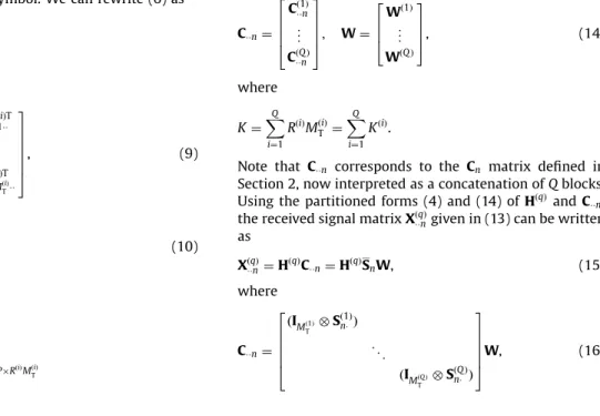
¼64ÞwithP¼K.

In order to illustrate the rate sharing characteristic of the proposed block ST spreading model, let us consider a system with Q ¼2 and MT¼2. The modulation has cardinality

m

¼16. Assume that the ST spreading blocks of both users have the same number of transmit antennas, i.e. Mð1Þ_T ¼Mð2Þ_T ¼1. Fig. 4 illustrates the theoretical (maximum) rate sharing between two users as the multiplexing factorRð1Þ_{of the first user is increased while} that of the second one is fixed atRð2Þ¼1 or 2. The rates are calculated using (20) with P satisfying the design requirement (19) in each case. First of all, note that the total rate

r

ð1Þ_þ

_r

ð2Þ_{is constant. The increase of}

_r

ð1Þ_comes at the expense of a decrease of

r

ð2Þ_{. The crossing of both} rate curves occurs whenRð1Þ

¼Rð2Þ

¼1 and 2. This figure

Table 1

User rates for several choices of the spatial spreading and multiplexing factors

fMð1Þ

T;Rð1Þg;_fM_Tð2Þ;Rð2Þ_g frð1Þ;rð2Þg rð1Þ=rð2Þ

f2;1g;_f1;1g f2;2g 1 f2;2g;_f1;1_{g f}2:4;1:2_g 2

f2;1g;_f1;2_{g f}1:5;3_g 1 2

f2;1g;_f2;1_{g f}1:5;1:5_g 1

f2;2g;f2;1g f2;1g 2

f2;3g;f2;1g f2:25;0:75g 3

f3;1g;f1;1g f1:5;1:5g 1

suggests that the rate of the different ST spreading blocks can be controlled by varying their multiplexing factors.

InFig. 5, we show the influence of the total number of transmit antennas on the achievable rate, for fixed multiplexing factors. We consider Q¼2, fRð1Þ;Rð2Þg ¼ f2;1g and

m

¼64. Users’ ST spreading blocks have the same number of transmit antennas in all the cases. As the number of transmit antennas used for spatial spreading is increased (so is the transmit diversity gain), the achiev-able rate of both users is decreased. Such a rate decrease comes from the fact thatPmust be increased according to the number of transmit antennas in order to satisfy (19).

5. Block-constrained received signal model

We formulate the received signal tensor (7) in equi-valent matrix forms associated with a block-constrained

tensor model. This model is a generalization of the constrained PARAFAC model proposed in [20–22], and we show how the constrained structure of this model is linked to the block ST spreading pattern at the transmitter. This model is a particular case of the block tensor model introduced in[28].

Recall the received signal model (15), where XðqÞ n2

C

MRP _{is viewed as the n-th slice of the received signal} tensor

X

₂

C

MRPN obtained by slicing it along its third dimension. Similarly, we define XðqÞ

mr2

C

PN _{and X}ðqÞ

p 2

C

NMR _{as them}

r-th andp-th slices obtained by slicing

X

along its first and second dimensions, respectively. Let us defineXðqÞ

1 ¼ ½Xð qÞT 1 Xð

qÞT NT2

C

NMRP_,XðqÞ

2 ¼ ½Xð qÞT 1 Xð

qÞT P

T

2

C

PNMR_andXðqÞ

3 ¼ ½Xð qÞT 1 Xð

qÞT

MRT2

C

MRPN_.

It can be shown that XðqÞ 1 , Xð

qÞ 2 and Xð

qÞ

3 admit the following constrained factorizations:

Xð₁qÞ¼ ðS

U

HðqÞ

_W

_{ÞW, (21)}

XðqÞ 2 ¼ ðW

T

S

U

ÞðHðqÞ

_W

_ÞT_{, (22)}

XðqÞ 3 ¼ ðHð

qÞ

_W

_WT

ÞðS

U

ÞT, (23)

where is the Khatri–Rao (column-wise Kronecker) product,HðqÞ _{is defined in (4),S¼ ½S}ð1Þ

SðQÞ_{, and}

_W

_,

_U

are block-diagonalconstraint matricesdefined by

W

¼

W

ð1Þ

. . .

W

ðQÞ

2 6 6 4

3 7 7

52

R

MTK, (24)

U

¼

U

ð1Þ

._. .

U

ðQÞ

2 6 6 4

3 7 7

52

R

RK, (25)

where theiri-th blocks have, respectively, the following Kronecker product structures:

W

ðiÞ¼I_MðiÞ

T 1 T

RðiÞ2

C

MðiÞ

TKð

iÞ

,

U

ðiÞ_¼1T

MðiÞ

T

I_RðiÞ2

C

R ðiÞ_KðiÞ

, (26)

with KðiÞ _{defined in (19). The demonstration of (21) is} provided in the Appendix.

6. Physical interpretation of

W

and

U

In the present context, the constraint matrices

_W

and

U

admit an interesting physical interpretation. They can be viewed assymbol-to-antenna loading matricesand their structure reveals the overall block ST spreading pattern considered at the transmitter. This interpretation sheds light on the different ST spreading designs that can be achieved by properly configuring these matrices with 1’s and 0’s. For example, let us consider MT¼3 transmit antennas and a transmission for Q¼2 users, which implies Q¼2 transmission blocks. Assume fMð1Þ_T ;Rð1Þg ¼ f2;1_g,_fMð2Þ_T ;Rð2Þ

g ¼ f1;3_g. From (24)–(26),

_W

and

_U

have

1 1.5 2 2.5 3 3.5 4

0.5 1 1.5 2 2.5 3 3.5

R(1)

Rate (bits/channel use)

Q = 2, M_T = 2, M_T = M_T = 1, μ = 16

User 1 (R(2) = 1) User 2 (R(2) = 1) User 1 (R(2) = 2) User 2 (R(2) = 2)

(1) (2)

Fig. 4.Rate sharing between two users.

2 4 6 8

0.5 1 1.5 2 2.5 3 3.5 4

M_T

Rate (bits/channel use)

Q = 2, {R(1)_{, R}(2)_{} = {2,1}, μ = 64}

User 1 User 2

the following structures:

W

¼

1 0 0 0 0

0 1 0 0 0

0 0 1 1 1

2 6 4

3 7 5;

U

¼

1 1 0 0 0

0 0 1 0 0

0 0 0 1 0

0 0 0 0 1

2 6 6 6 4

3 7 7 7 5.

First, note that both

W

and

U

are block-diagonal matrices with two diagonal blocks, i.e.:

f

W

ð1Þ;

W

ð2Þg ¼ fI2;1T3g; f

U

ð1Þ;

U

ð2Þg ¼ f1T2;I3g.

Each row of

W

defines the multiplexing factor at each transmit antenna. The number of 1’s entries in each row of

W

defines the number of symbols combined into each transmit antenna. Observe that the first and second rows of

W

(both associated with the first transmission block) have only one non-zero entry, which indicates that both transmit antennas of this block transmit only one symbol at a time. The third row contains three non-zero entries, meaning that three symbols are simultaneously trans-mitted by the antenna of the second block.

Now, let us look at the structure of

U

. Its number of rows corresponds to the total number of multiplexed data streams. Each row of

_U

defines thespatial spreading factor associated with each data stream: The number of 1’s entries in each row of

U

defines the number of antennas used to transmit each data stream. Note that its first row has two non-zero entries, which means that the first data stream is spread over the two first transmit antennas. The three other rows have only one non-zero entry, which indicates that the three other data streams are trans-mitted using only one transmit antenna, i.e. they are not spatially spread at the transmitter. The chosen spreading-multiplexing configuration can be checked by means of the following matrix:

WU

T¼

1 0 0 0

1 0 0 0

0 1 1 1

2 6 4

3 7

52

C

MTR.

This matrix product reveals the joint spreading-multi-plexing pattern. For a fixed row, one can check for the number of data streams multiplexed at a given antenna by counting the number of 1’s entries in that row. On the other hand, for a fixed column, one can check for the number of antennas over which a given data stream is spread.

7. Receiver algorithm

As mentioned in the last section, the choice of a semi-unitary (Vandermonde) matrixWallows the separation of users’ transmissions deterministically, so that the detec-tion of the transmitted data can be carried out indepen-dently for each user. In the following, we exploit the knowledge and structure of W for MUI elimination and then the tensor structure of the received signal for a blind joint channel estimation and symbol recovery.

7.1. MUI elimination

The first processing step at each receiver performs a deterministic MUI elimination, by relying on the structure of the unfolded spreading matrixW2

C

KPand assuming KpP. Let us defineFðqÞ_¼WðqÞH ₂

C

PKð

qÞ

as theq-th user receive filter. For the q-th user, the elimination of the MUI coming from the transmission blocks f1;. . .;q1;

qþ1;. . .;Qg, consists in post-multiplying the received

signal matrixXð₁qÞgiven in (21) byFðqÞ_{, which gives}

Yð₁qÞ¼Xð₁qÞFðqÞ_{¼ ðS}

_U

_HðqÞ

_W

_ÞDðqÞ_{, (27)}

where

DðqÞ_¼WFðqÞ_¼

0_Kðq1Þ_KðqÞ

I_KðqÞ

0_ðKKðqÞ_ÞKðqÞ

2 6 6 4

3 7 7 52

C

KK

ðqÞ

, (28)

with

KðqÞ_¼Xq

i¼1

KðiÞ_.

Note that all the blocks inDðqÞ_{except the one} correspond-ing to theq-th user are zero. This allows us to rewrite (27) as a MUI-free model:

YðqÞ 1 ¼ ðSð

qÞ

_U

ðqÞ_Hðq;qÞ

_W

ðqÞ_ÞI

KðqÞ, (29)

which can be viewed as a single-user tensor model with constrained structure. Therefore, Yð₁qÞ is an unfolded matrix of a tensor

Y

ðqÞ₂

C

MRKðqÞ_N

resulting from a linear transformation of the received signal tensor

X

ðqÞ ₂

C

MRPN by the associated receive filter FðqÞ₂

C

PKðqÞ as shown in (27). A one-to-one correspondence between the multiuser and single-user tensor models can be obtained by comparing Xð₁qÞ in (21) with Yð₁qÞ in (29). This correspondence is

ðHðqÞ_;S;W;

_W;

_U

_{Þ ! ðH}ðq;qÞ_;SðqÞ_;I

KðqÞ;

W

ðqÞ;

U

ðqÞÞ.

By analogy with (22) and (23), we can also represent the information contained in YðqÞ

1 by means of two other unfolded matrices:

Yð₂qÞ¼ ðI_KðqÞSðqÞ

U

ðqÞÞðHðq;qÞ

W

ðqÞÞT, (30)

Yð₃qÞ¼ ðHðq;qÞ

_W

ðqÞ

I_KðqÞÞðSðqÞ

U

ðqÞÞT. (31)

Note that YðqÞ

2 2

C

KðqÞ_NMR

and YðqÞ

3 2

C

MRKðqÞ_N

are ‘‘re-shaped’’ versions ofYðqÞ

1 2

C

NMRKðqÞ

. Defining

Z2ðSðqÞÞ ¼ ðIKðqÞSðqÞ

U

ðqÞÞ

W

ðqÞT2

C

K ðqÞ_NMðqÞ

T _{, (32)}

Z3ðHðq;qÞÞ ¼ ðHðq;qÞ

W

ðqÞIKðqÞÞ

U

ðqÞT2

C

MRK ðqÞ_RðqÞ

, (33)

we can rewriteYð₂qÞandYð₃qÞas

YðqÞ

7.2. Identifiability

For studying the identifiability of model (34), let us make the following assumptions concerning the structure ofSðqÞ_andHðq;qÞ_:

(A1) ‘‘Persistence of excitation’’ of the transmitted sym-bols which implies, in our context, thatSðqÞ _{can be} considered as a full column-rank matrix with probability one ifNis large enough.

(A2) An ‘‘ideal’’ MIMO channel so that the entries of the channel matrix are assumed to be independent and randomly drawn from an absolutely continuous distribution, which implies that Hðq;qÞ _{is full rank} with probability one.

Under assumptions (A1)–(A2), joint channel–symbol identifiability from the MUI-free model defined in (34) requires thatZ2ðSðqÞÞandZ3ðHðq;qÞÞin (32) and (33) be full column-rank, since these matrices must have a left-inverse. Let us study the rank properties of Z2ðSðqÞÞ and

Z3ðHðq;qÞÞ. We make use of the concept of k-rank [15], which is recalled here for convenience:

Definition 1. Thek-rank ofA2

C

IF_{, is equal tok}

Aifany

set ofk_Acolumns ofAis independent, but there exists a set ofkAþ1 linearly dependent columns inA. We have

kAprank_ðA_Þpmin_ðI;FÞ.

We have to note that if two columns inAare repeated, and ifA does not contain a zero column, then we have kA¼1. Let us also recall the two following lemmas: Lemma 1 (k-rank of the Khari–Rao product[35]). Suppose

that A2

C

IF andB2

C

JF are such that kAX1and kBX1

(i.e. neitherAnorBhas a zero column).If kAþkB¼Fþ1,

thenABis full column-rank.

Lemma 2. If A is full column-rank, then we have rankðABÞ ¼rankðBÞ.

Taking the definitions (26) of

_W

ðqÞ_and

U

ðqÞinto account, we have

W

ðqÞ¼

1T_RðqÞ

. . .

1T_RðqÞ

2 6 6 6 6 4

3 7 7 7 7 5 |fflfflfflfflfflfflfflfflfflfflfflfflfflfflfflffl{zfflfflfflfflfflfflfflfflfflfflfflfflfflfflfflffl}

MðqÞ

T times

)rank_ð

_W

ðqÞ

Þ ¼MðqÞ

T ,

U

ðqÞ_{¼ ½I}

RðqÞ I_RðqÞ

|fflfflfflfflfflfflfflffl{zfflfflfflfflfflfflfflffl}

MðqÞ

T times

)rank_ð

_U

ðqÞ_{Þ ¼R}ðqÞ_,

which implies that

_W

ðqÞ _and

U

ðqÞ be full row-rank. From these expressions of

W

ðqÞ_and

_U

ðqÞ_{, we get}

SðqÞ

_U

ðqÞ_{¼ ½S}ðqÞ _SðqÞ

|fflfflfflfflfflfflfflffl{zfflfflfflfflfflfflfflffl}

MðqÞ

T times

and

Hðq;qÞ

_W

ðqÞ_{¼ ½H}ðq;qÞ 1 Hð

q;qÞ 1

|fflfflfflfflfflfflfflfflfflffl{zfflfflfflfflfflfflfflfflfflffl}

RðqÞ_times

Hðq;qÞ MðqÞ

T

Hðq;qÞ MðqÞ

T

|fflfflfflfflfflfflfflfflfflfflffl{zfflfflfflfflfflfflfflfflfflfflffl}

RðqÞ_times

,

which implies that

k_SðqÞ_UðqÞ¼k_Hðq;qÞ_WðqÞ¼1.

As we havekI_KðqÞþkSðqÞ_UðqÞ¼KðqÞþ1, application of Lemma

1 to the Khatri–Rao product in (32) implies that I_KðqÞ

SðqÞ

_U

ðqÞ_{be full column-rank, i.e. rankðI}

KðqÞSðqÞ

U

ðqÞÞ ¼KðqÞ.

Application of Lemma 2 leads to rankðZ2ðSðqÞÞÞ ¼ rank_ð

_W

ðqÞT

Þ ¼rank_ð

_W

ðqÞ

Þ ¼MðqÞ

T , i.e.Z2ðSðqÞÞis full column-rank. The same reasoning applies for showing that Z3ðHðq;qÞÞis also full column-rank.

7.3. Blind joint channel and symbol recovery

After MUI elimination at each receiver, we propose to apply the classical alternating least squares (ALS) algo-rithm on the resulting interference-free tensor model (34), in order to blindly recover the transmitted symbols jointly with channel estimation. The ALS algorithm consists in an alternate estimation of the unknown matricesHðq;qÞ _and

SðqÞ_{,q¼1;. . .;Q. At each iteration, one matrix is estimated} in the least squares sense while the other one is fixed to its value obtained at the previous estimation step. The algorithm is initialized using a random valuebSð_tq_¼0Þ . At the t-th iteration, the two least-squares update equations are

b

Hðq;qÞT

t ¼ ½Z2ðbSðtq1ÞÞyYð

qÞ

2 , (35)

b

SðqÞT

t ¼ ½Z3ðHbtðq;qÞÞyYð3qÞ, (36)

whereydenotes the pseudo-inverse. For theq-th receiver, the following error measure is computed at the t-th iteration:

eðqÞ

t ¼ kYð1qÞ ðbSð

qÞ

t

U

ðqÞHbðq

;qÞ

t

W

ðqÞÞkF, (37)

wherek kFdenotes the Frobenius norm. We choosejeðtqÞ

eðqÞ

t1jp10

6 _{as the convergence threshold, q}

¼1;. . .;Q.

The estimation of both Hðq;qÞ _{and S}ðqÞ _{is affected by a} scaling ambiguity. In other words, the columns of the estimated channel and symbol matrices are affected by unknown scaling factors that compensate each other. Following [23], we eliminate this scaling ambiguity by assuming that the first transmitted symbol of each data stream is equal to one, which corresponds to have all the elements in the first row of S equal to one. Thus, we eliminate the scaling ambiguity by normalizing each column ofbSby its first element yielding

e

SðqÞ 1 ¼bSð

qÞ

1D11 ðbSð1qÞÞ, wherebSðqÞ

1 corresponds to the estimated value obtained after convergence andD1ðÞdenotes the diagonal matrix formed from the first row of its matrix argument. After such a normalization, we obtain a final estimate of the channel matrix without scaling ambiguity using (35):

e

Hðq;qÞT

1 ¼ ½Z2ðeSð1qÞÞyYð qÞ 2 .

Discussion: In this work, we have modeled the channel

different relative propagation delays. In this scenario, we can still work with the proposed block ST spreading model by assuming that the spreading codes are augmented by a number of trailing zeros, or ‘‘guard chips’’ in order to avoid inter-symbol interference. The main impact is that, in this case, the spreading matrixWisunknownat the receiver due to the convolution of the transmitted spreading codes with the impulse response of the multipath channel. Since the orthogonality between the transmitted data streams is destroyed by multipath propagation, the two-steps receiver algorithm ðMUI eliminationþALSÞ should be replaced by a MU detection receiver based on the classical three-steps ALS algorithm where thechannel,symboland

spreadingmatrices are iteratively estimated[15]. The price

to pay is, of course, the increased complexity of the receiver algorithm.

8. Simulation results

In this section, the performance of the proposed block ST spreading-based MU-MIMO system using the ALS algorithm is illustrated by means of computer simula-tions. The number of Monte Carlo runs vary from 1000 to 5000 depending on the simulated SNR value. At each run, the noise power is generated according to the sample SNR value given by SNR¼10 log₁₀ðkXðqÞ

1 k2F=kV1ðqÞk2FÞ, whereVð1qÞ represents the additive noise matrix. A Rayleigh fading MIMO channel is assumed. The elements of the channel matrix HðqÞ _{are i.i.d. samples of a complex Gaussian} process with zero mean and unit variance. Each run represents a different realization of the MIMO channel and the transmitted symbols are drawn from a pseudo-random QPSK or QAM sequence. The BER curves represent the performance averaged on the transmitted data

streams. In all the results, we focus on system configura-tions with a small number MR of receive antennas

ðMRpM_Tis generally assumed). For clarity of presentation, we considerQ ¼1;2 or 3 users. Unless otherwise stated, we considerN¼10 andP¼Kin order to satisfy (19). In some simulations, we focus on the individual performance of each user by averaging the performance over the data streams of each user. In some others, the performance is averaged over all the transmitted data streams of all the users.

8.1. BER performance

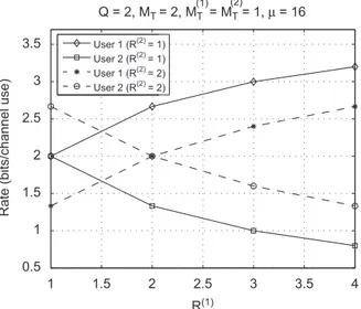
We begin by evaluating the BER performance of the block ST spreading-based MU-MIMO system using the ALS algorithm. We consider a two-users systemðQ¼2Þwith corresponding transmission blocks parameterized by

fMð1Þ_T ;Rð1Þ_{g ¼ f1;2g and fM}ð2Þ

T ;Rð2Þg ¼ f2;2g. A time-slot

containingN¼10 symbols is processed at the receiver. QPSK modulation is usedð

m

¼4Þ. Unless otherwise stated, we assumeP¼Mð1Þ_T Rð1Þ_þMð2Þ

T Rð2Þ in order to satisfy the requirement (19) for maximum transmit diversity. In this case we haveP¼6 and both users have the same rate

r

ð1Þ_¼

_r

ð2Þ_¼2

3 bits per channel use. A single transmit antenna is used to transmit the two data streams of the first user, while two transmit antennas are dedicated to the second user.Fig. 6shows the individual performance of each user assumingMR¼1 and 2 receive antennas. We can clearly see that the second user has an improved performance over the first one, due to a higher transmit diversity gain obtained by spreading the data streams across two transmit antennas.

Now, we investigate the influence of the spreading factorPon the receiver performance. We assumeQ¼1

0 3 6 9 12 15 18

10−4 10−3 10−2 10−1 100

SNR (dB)

BER

Q = 2, {M_T, R(1)_{} = {1,2}, {M}

T, R(2)} = {2,2}, N = 10, QPSK

User 1 (M_R=1)

User 1 (MR=2)

User 2 (MR=1)

User 2 (MR=2)

(1) (2)

(single-user/single-block case) and consider two ST spreading configurations _fMT;Rg ¼ f2;2g and fMT;Rg ¼

f4;2g. As shown in Fig. 7, for fMT;Rg ¼ f2;2g, the BER performance is degraded withP¼3 (note thatP¼3 does not satisfy (19)) in comparison withP_¼4 (thus satisfying (19)). The same comment is valid forP¼6 with respect to P¼8 for fMT;Rg ¼ f4;2g. The BER floor observed in the figure is due to the lack of orthogonality between theR¼

2 transmitted data streams whenPdoes not satisfy (19). Note that, in this case, Eq. (28) is no more valid, which means that multiple-access interference remains present at the receiver, then causing irreducible estimation/ detection errors. The BER floor can be interpreted in terms of residual interference. Such a performance degradation comes with only a marginal increase in rate. Indeed, the rate is

r

¼4

3 for P¼3 and

r

¼1 for P¼4. These results confirm that the receiver performance is sensitive to the spreading factor.

In Fig. 8, we compare block ST spreading with KRST coding [23]. We consider MT¼4, MR¼2 and 16-QAM. Different ST spreading configurations are simulated by varying the number of ST spreading blocks/users. We consider the following cases: (i) Q¼3 with

fMð1Þ_T ;Mð2Þ_T ;Mð3Þ_T g ¼ f2;1;1g, (ii) Q¼2 with fMð1Þ_T ;Mð2Þ_T g ¼

f2;2g, (iii)Q¼1 withfMTg ¼4. Note that KRST coding is a special case of the proposed approach for Q¼MT¼4 (constellation rotation is not considered here for simulat-ing KRST codsimulat-ing). KRST codsimulat-ing provides the best perfor-mance in terms of rate, but the worst perforperfor-mance in terms of BER. In the proposed approach, by decreasing the number of ST spreading blocks, the BER performance is improved since more transmit antennas are used for each block to achieve higher transmit diversity gains. The performance improvement is also linked to the receiver algorithm, since the blind separation of the transmitted data streams improves as Q decreases. It is worth mentioning, however, that such an improvement comes at the expense of a decrease in rate.

Fig. 9compares the proposed MIMO system with the Alamouti code[6]in the particular single-user case with Q_¼1, MT¼MR¼2 and R¼2. For the Alamouti code, perfect channel knowledge is assumed at the receiver, contrarily to our system which uses blind detection. In order to keep the same rate (1 bit/channel use) for a fair comparison, the Alamouti code uses BPSK while the proposed MIMO system uses QPSK. The performance gap between the proposed approach and the Alamouti code is 3 dB for a BER of 2103_{. The slope of the BER curves} indicates that both approaches have the same diversity gain.

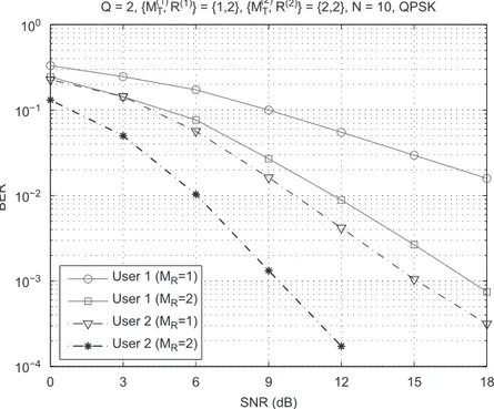
8.2. RMSE performance

In the next experiment, we investigate the accuracy of the ALS algorithm in recovering the channel and symbol matrices. The fixed simulation parameters are Q_¼1,

0 3 6 9 12 15 18

10−4 10−3 10−2 10−1 100

SNR (dB)

BER

Q = 1, M_R = 2, N = 10, QPSK

{MT,R} = {2,2}, P = 3 {MT,R} = {2,2}, P = 4 {MT,R} = {4,2}, P = 6 {MT,R} = {4,2}, P = 8

Fig. 7.BER versus SNR for different values ofP, usingfMT;Rg ¼ f2;2gand

f4;2g.

0 3 6 9 12 15 18

10−4 10−3 10−2 10−1 100

SNR (dB)

BER

M = 2, N = 10, 16−QAM

KRST coding, Q = M = 4

Rate = 4

Rate = 3

Rate = 2

Rate = 1

Fig. 8.Comparison of block space–time spreading with KRST coding [23].

−6 −3 0 3 6 9

10−5

10−4

10−3

10−2

10−1

100

SNR (dB)

BER

N = 10

MT¼2, R¼1, MR¼2. The evaluation is based on the root-mean-square error (RMSE) between the estimated and true matrices calculated according to the following formulae:

RMSE_ðSÞ ¼

ffiffiffiffiffiffiffiffiffiffiffiffiffiffiffiffiffiffiffiffiffiffiffiffiffiffiffiffiffiffiffiffiffiffiffiffiffiffiffiffiffiffiffiffi

1 LNR

XL

l¼1

kbS1ðlÞ Sk2F

v u u

t ,

RMSEðHÞ ¼

ffiffiffiffiffiffiffiffiffiffiffiffiffiffiffiffiffiffiffiffiffiffiffiffiffiffiffiffiffiffiffiffiffiffiffiffiffiffiffiffiffiffiffiffiffiffiffiffiffiffiffiffiffi

1

LMTMR

XL

l¼1

kHb₁ðlÞ Hk2F

v u u

t ,

whereLis the number of Monte Carlo runs, whilebS1ðlÞ andHb1ðlÞare the estimated matrices after convergence at the l-th run. In this experiment, we assume L¼1000.

Fig. 10shows that the RMSE associated with the estima-tion of the transmitted symbols exhibits a linear decrease as a function of the SNR. Estimation accuracy also improves asNincreases.

In Fig. 11, the RMSE associated with the channel estimation is depicted for different numbers MT of

transmit antennas with Q¼1, R¼2, MR¼2 and

N¼10. Improved estimation of the channel matrix is obtained as MT is increased. Note that, despite the increase of the number of channel parameters to be estimated whenMTincreases, this performance improve-ment is attributed to the higher transmit diversity gain.

8.3. Throughput performance

In this section, the average throughput of the proposed MU-MIMO system is studied for some system configura-tions. Our aim is to show that the block ST spreading model covers different ‘‘transmission modes’’ that could be adapted according to the SNR in a practical transmis-sion setting. Throughput results are interesting from a practical point of view, since they provide a more realistic insight on the physical-layer performance of the proposed receiver strategy.

In order to obtain block error rate (BLER) measures for throughput calculation, we introduce an 8-bit cyclic redundancy check (CRC) scheme at each data block, which is defined as a collection ofNRsymbols (Nsymbols per data streamRdata streams). We only vary the temporal spreading factorPwhich can be viewed as a parameter controlling the redundancy of the transmitted symbols in the time domain. The average values for the BLER are calculated over 1000 independent runs for each SNR value. No channel coding is used. The calculation of the total throughput

G

(summed over theQ users) is made using the following formula:

G

¼X

Q

q¼1

G

ðqÞ

¼X

Q

q¼1

ð1BLERðqÞ_Þ

_r

ðqÞ _ðbits=T

blockÞ,

where BLERðqÞ _{is the q-th user BLER,}

_r

ðqÞ _{is the nominal} rate of the q-th transmission block defined in (20), and Tblock¼NRTs denotes the duration of one transmission block of NR symbols, Ts being the symbol period. The number of symbols per data stream is fixed atN¼10. It is worth noting that the plotted throughput performances do not reflect the bandwidth expansion due to the transmission of known symbols that is necessary for eliminating the scaling ambiguity in the ALS algorithm.

InFig. 12, we considerQ ¼2 users withfMð1Þ_T ;Rð1Þg ¼ f2;1_gand_fMð2Þ_T ;Rð2Þ

g ¼ f1;1_g. Note that both users have the

same multiplexing factor (thus the same nominal rate) but different spatial spreading factors. In this figure, we evaluate the individual throughput performance of each user. Each user throughput curve is reproduced for two values of P. In the first case, we have P¼Mð1Þ_T Rð1Þþ

Mð2Þ

T Rð2Þ¼3. In the second case,P¼2 is assumed, which is below the required value for achieving the maximum transmit diversity gain. Considering firstP¼3, we verify fromFig. 12that the expected transmit diversity gain of the first user is effectively translated into a higher throughput gain with respect to the second user. When Pis decreased, we observe an increase in the first user’s throughput for medium-to-high SNR levels, while, for low

0 5 10 15 20 25 30 35 40

10−3

10−2

10−1

100

SNR (dB)

RMSE (symbol)

Q = 1, MT = 2, R = 1, MR = 2, QPSK

N = 5 N = 10 N = 20 N = 50

Fig. 10.Symbol RMSE for different values ofN.

0 5 10 15 20 25 30 35 40

10−3

10−2

10−1

100

SNR (dB)

RMSE (channel)

Q = 1, R = 2, MR = 2, N = 10, QPSK

MT = 2 MT = 3 M_T = 4 M_T = 5

SNR levels, a throughput loss is observed. Therefore, the diversity loss that occurs when P is decreased is compensated by a throughput gain, especially for high SNR levels. For the second user, where no transmit diversity is available, a significant degradation in the throughput performance is observed.

Fig. 13shows a set of throughput curves for different values ofPconsidering a single-user system withMT¼4,

R¼4, MR¼2, and using 16-QAM. This figure indicates that it is possible to obtain a variable throughput performance by adjusting P according to the SNR. Otherwise stated, this experiment suggests that a sort of

link adaptation could be implemented by varying the

temporal spreading factor P in order to keep the best throughput within each SNR region. In this case, the switching points between different values ofPare at an SNR of 15, 21 and 28 dB.

9. Conclusion and perspectives

In this paper, we have proposed a new block space– time spreading model for the downlink of MU-MIMO system based on tensor modeling. In the proposed approach, multiple users are associated with different transmission blocks, each block grouping a different set of transmit antennas. Within each transmission block, space–time spreading is formulated as a third-order tensor transformation. The core of this transformation is modeled by means of a 3-D spreading code tensorthat jointly spreads and combines independent data streams across multiple transmit antennas. We have formulated the received signal as a block-constrained tensor model, which is characterized by two fixed constraint matrices revealing the overall space–time spreading pattern con-sidered at the transmitter. The proposed approach is flexible in the sense that it allows different spatial spreading factors (diversity gains) as well as different multiplexing factors (code rates) for the users. At the receiver, deterministic MUI interference is performed by each user, followed by a blind joint channel and symbol recovery stage using the ALS algorithm. Simulation results have shown that the block space–time spreading-based MU-MIMO system can achieve variable BER and through-put performances by adjusting the three transmit para-meters which are thespatial spreading, multiplexingand

temporal spreading factors. A perspective of this work

−6 −3 0 3 6 9 12 15 18 21

0 0.1 0.2 0.3 0.4 0.5 0.6 0.7 0.8 0.9

SNR (dB)

Throughput (bits / T

block

)

Q = 2, { M_T, R(1)_{} = {2,1}, {M}

T, R(2)} = {1,1}, MR = 2, N = 10, QPSK

User 1 (P = 3) User 2 (P = 3) User 1 (P = 2) User 2 (P = 2)

(1) (2)

Fig. 12.Per-user throughput performance forP¼2 and 3.

3 6 9 12 15 18 21 24 27 30 33 36 39

0 0.2 0.4 0.6 0.8 1 1.2 1.4 1.6 1.8 2

SNR (dB)

Throughput (bits / T

block

)

Q = 1, MT = 4, R = 4, MR = 2, N = 10, 16−QAM

P = 16 P = 12 P = 10 P = 8