Space–time spreading–multiplexing for MIMO wireless communication system susingthe PARATUCK2 tensor model art timespreading

Space–time spreading–multiplexing for MIMO wireless

communication systems using the PARATUCK-2 tensor model

$

Andre´ L.F. de Almeida

a,b

_{, Ge´rard Favier}

a,

_{, Joa˜o C.M. Mota}

b a_{I3S Laboratory, University of Nice-Sophia Antipolis, CNRS, France}

b_{GTEL-Wireless Telecom Research Group, Federal University of Ceara´, Fortaleza, Brazil}

a r t i c l e

i n f o

Article history:

Received 28 October 2008 Received in revised form 16 February 2009 Accepted 16 April 2009 Available online 3 May 2009

Keywords:

MIMO systems Space–time spreading Multiplexing Blind detection Tensor modeling PARATUCK-2 model

a b s t r a c t

In this paper, we present a new space–time spreading–multiplexing model for multiple-input multiple-output (MIMO) wireless communication systems relying on a tensor modeling of the transmitted and received signals. At the transmitter, we exploit the core of a PARATUCK-2 tensor model composed of a precoding matrix and two allocation matrices that allow to control the spreading and multiplexing of the data streams across the space dimension (transmit antennas) and time-dimension (time-slots). Different MIMO schemes combining space–time multiplexing and diversity can be derived from the proposed model. The identifiability and uniqueness of the PARATUCK-2 tensor model for the received signal are discussed and subsequently exploited for a joint blind channel estimation and symbol detection. The bit-error-rate performance of different transmit schemes derived from the proposed tensor model is evaluated by means of computer simulations.

&2009 Elsevier B.V. All rights reserved.

1. Introduction

It is well known for some time that multiple-input multiple-output (MIMO) wireless communication sys-tems employing multiple antennas at both the transmitter and the receiver provide multiplexing gains [1] and/or diversity gains [2] to increase the data rate (i.e. higher spectral efficiency) and/or the reliability of the transmis-sion (i.e. lower error rate) without additional bandwidth. In order to provide multiple-accessing capabilities to MIMO systems, several approaches make use of code-division multiple-access (CDMA) technology by associat-ing multiple transmit antennas and multiple user signals

to orthogonal spreading transforms in different manners

[3,4]. Optionally, when current channel state is known in advance at the transmitter, some form of precoding can also be used to improve system performance[5].

The use of tensor decompositions for modeling MIMO transceivers with blind signal processing has been addressed in several recent works[6,8–12]. The approach of Sidiropoulos and Budampati[6], therein calledKhatri– Rao space–time (KRST) codes, relies on a PARAllel FACtor (PARAFAC) model[7]. By precoding each data stream over multiple symbol periods, a joint blind channel estimation and symbol detection is afforded by means of a PARAFAC

modeling of the received signal tensor. The work [8]

presents a generalized block-tensor model for multiple-access MIMO transceivers. The common feature of the solutions [6] and [8] is the use of pure spatial multi-plexing, where each data stream is transmitted by a single transmit antenna and coded across the time-dimension only. Consequently, no transmit spatial diversity is allowed and the number of data streams is restricted to be equal to the number of transmit antennas. To overcome

Contents lists available atScienceDirect

journal homepage:www.elsevier.com/locate/sigpro

Signal Processing

0165-1684/$ - see front matter&2009 Elsevier B.V. All rights reserved.

doi:10.1016/j.sigpro.2009.04.028

$

This paper is an extended version of our conference paper presented at EUSIPCO’08 and entitled ‘‘Space–Time Spreading–Multiplexing for MIMO Antenna Systems with Blind Detection using the PARATUCK-2 Tensor Model’’. This work was supported by CAPES-COFECUB, project no Ma 544/07.

_{Corresponding author. Tel.: +33 492 942 736; fax: +33 492 942 896.}

E-mail addresses:andre@gtel.ufc.br (A.L.F. de Almeida),

this limitation, the work in[9]uses a constrained tensor model which can be viewed as a ‘‘structured’’ PARAFAC model with ana prioriknown model structure. This allows to model, in addition to spatial multiplexing, a wider class of MIMO transmissions characterized by a joint space and time spreading. In order to cope with multiuser downlink transmissions, de Almeida et al.[10]formulated a block-constrained version of the tensor model of [9], which allows a multiuser space–time transmission with different spatial spreading factors (diversity gains) as well as different multiplexing factors (code rates) for the users.

More general space–time spreading structures were recently proposed relying on a third-order CONstrained FACtor (CONFAC) tensor model[11,12]. The approach of de Almeida et al. [11] introduces two constraint matrices withvariable1’s and 0’s structure into the tensor model. These constraint matrices are referred therein as stream and codeallocation matrices. As opposed to the approach of[9,10]where the two constraint matrices have a fixed structure, in[11]the structure of the constraint matrices can be controlled to design transmit schemes with different spatial multiplexing, code multiplexing and transmit antenna assignments for the data streams. The work [12] further generalizes [11] by including a third allocation matrix that defines the mapping of the precoded signals to the transmit antennas. In this case, the constrained structure of the CONFAC model is fully exploited at the transmitter (for designing finite-sets of MIMO transmission schemes) as well as at the receiver (for blind signal processing).

In this work, we present a novel tensor-based space– time spreading–multiplexing model. At the transmitter, we exploit the structure of a PARATUCK-2 tensor model to design different precoder structures combining space– time multiplexing and diversity. The heart of the proposed tensor model is composed of two constraint matrices. These constraint matrices play the role of stream-to-slot and antenna-to-slot allocation matrices. Differently to the

CONFAC model of de Almeida et al. [11,12], the two

allocation matrices of the PARATUCK-2 core tensor jointly control the spatial and temporal allocations, i.e. the allocations of data streams to transmit antennas and time-slots. Moreover, the number of channel uses asso-ciated with the transmission of each data stream may be different from one data stream to another. Such a feature is not possible with the existing tensor-based space–time transmission models and is intrinsic to the PARATUCK-2 modeling. At the receiver, we capitalize on the structure of the PARATUCK-2 model for the received signal to perform a joint blind detection and channel estimation. The identifiability issue of the proposed tensor model is discussed and a simple blind receiver based on the alternating least squares (ALS) algorithm is presented.

The PARATUCK-2 model can be viewed as a general-ization of the PARAFAC one. It mixes the properties of both PARAFAC[7]and TUCKER-2[13]models. Consequently, it allows the flexibility of TUCKER-2 model while retaining PARAFAC’s uniqueness properties. This model has been studied in the psychometrics literature [14]and subse-quently exploited by Bro[15]to solve special data analysis problems in chemometrics. The first application of

PARATUCK-2 in signal processing was proposed by Kibangou and Favier[16]for the blind joint identification and equalization of Wiener–Hammerstein communica-tion channels. The present paper shows that this model is also useful to model the transmitted and received signals in MIMO wireless communication systems while afford-ing a blind signal processafford-ing.

Despite the differences among PARAFAC, CONFAC and PARATUCK-2 modeling approaches, it is worth mentioning that they share common characteristics. First, they simul-taneously exploit three diversity dimensions (space, time

andcode) that characterize the received signal tensor. Each diversity dimension is associated with a different matrix factor of the received signal tensor model as follows:

Thespace dimensionis created by the multiple-antenna channel and is associated with thechannel matrix.

The time dimension arises by collecting the received signal during several symbol periods and is associated with thesymbol matrix.

The code dimension is generated by precoding each transmitted symbol across multiple time-slots, and is associated with theprecoder matrix.

The relationship involving channel, symbol and precoder matrices depends on the structure adopted to model the received signal tensor. In this work, such a relationship is defined by the PARATUCK-2 structure. The use of this tensor modeling allows to perform a blind joint symbol and channel estimation under identifiability conditions more relaxed than those of conventional matrix modeling based approaches, and without requiring statistical independence between transmitted signals. Instead, the receiver signal processing is deterministic and directly exploits the known structure of the received signal tensor. Moreover, tensor-based receivers are generally based on a joint detection of the transmitted signals (either from different users or from multiple transmit antennas).

We emphasize that the contribution of this work concerns both transmitter and receiver processing. At the transmitter, the PARATUCK-2 model structure is used to model space– time multiplexing–spreading. At the receiver, this structure is exploited to blindly estimate the transmitted symbols and the MIMO channel.Fig. 1provides an illustration of the use of tensor models in a MIMO communication chain. The three signal dimensions that generally appear at the transmitter and receiver are highlighted.

are presented in Section 7 to illustrate the performance of this blind receiver. This paper is concluded in Section 8.

Notations: Some notations and properties are now defined.AT_,A1 _andAy _{stand for transpose, inverse and}

pseudo-inverse of A, respectively. The operator diagðaÞ

forms a diagonal matrix from its vector argument, while

DiðAÞforms a diagonal matrix holding thei-th row ofAon

its main diagonal. The Kronecker and the Khatri–Rao products are denoted byand, respectively,

AB¼ ½A1B1;. . .;ARBR ¼

BD1ðAÞ . . .

BDIðAÞ

2 6 6 4

3 7 7

5 (1)

withA¼ ½A1;. . .;AR 2

C

IR,B¼ ½B1;. . .;BR 2

C

JR. We

shall make use of the following property of the Kronecker product:

vecðACBTÞ ¼ ðBAÞvecðCÞ. (2) forA2

C

IR,B2

C

JS, andC2

C

RS. Scalars are denoted by lower case lettersða;b;. . ._;

a

;

b

;. . .Þ, vectors are written as boldface lower case lettersða;b;. . .Þ, matrices as boldface capitals ðA;B;. . .Þ, and tensors as calligraphic letters

ð

A

_;

B

_;. . .Þ.

2. Main third-order tensor models

This section gives a brief overview of the main third-order tensor models: the PARAFAC, TUCKER-3, PARATUCK-2 and CONFAC tensor models. The constrained PARATUCK-2 model used in this work is more particularly detailed.

2.1. PARAFAC

The PARAllel FACtor model of

X

₂

C

I1I2I3 _{has the}

following scalar form:

xi1;i2;i3¼

XF f¼1

ai1;fbi2;fci3;f, (3)

whereai1;f¼ ½Ai1;f,bi2;f¼ ½Bi2;f andci3;f¼ ½Ci3;f are scalar

components of the three matrix factors A2

C

I1F

, B2

C

I2F_andC2

_C

I3F_{, respectively, andFdefines the rank of}

the tensor.

2.2. TUCKER-3

The TUCKER-3 model was proposed by Tucker in the 1960s[13]. It incorporates most of the other third-order tensor models as special cases, and it can be written in scalar form as

xi1;i2;i3¼

XR1

r1¼1

XR2

r2¼1

XR3

r3¼1

ai1;r1bi2;r2ci3;r3gr1;r2;r3, (4)

where ai1;r1¼ ½Ai1;r1, bi2;r2¼ ½Bi2;r2 and ci3;r3¼ ½Ci3;r3 are

scalar components of the three matrix factorsA2

C

I1R1_,

B2

C

I2R2 _{and C2}

_C

I3R3_{, respectively, and g}

r1;r2;r3¼

½

G

r1;r2;r3 is a scalar component of the TUCKER-3 core

tensor

G

2

C

R1R2R3_.

It is worth noting that TUCKER-3 reduces to PARAFAC in the caseR1¼R2¼R3¼Fwithgf;f;f¼

d

f;f;f, where

d

f;f;f

is the Kronecker delta. In other words, PARAFAC is a special case of TUCKER-3 with a diagonal core tensor, the main diagonal being composed of ones.

Special cases: TUCKER-2and TUCKER-1: The TUCKER-2 model arises from the TUCKER-3 one by setting one matrix factor, sayC, to the identity matrix. This model is therefore defined as

xi1;i2;i3¼

XR1

r1¼1

XR2

r2¼1

ai1;r1bi2;r2gr1;r2;i3, (5)

where gr1;r2;i3 is the scalar component of the TUCKER-2

core tensor

G

2

C

R1R2I3_{. Similarly, the TUCKER-1 model}

arises from the TUCKER-3 one by setting two matrix factors, say B and C, to identity matrices. In this case,

TX signal tensor Input data

streams

Transmitter processing (precoding)

RX signal tensor

MIMO channel

Receiver processing (signal separation) Joint blind

symbol and channel estimation

Tensor models (PARAFAC, CONFAC,

PARATUCK-2,...)

Space Dimension

(Tx)

Time dimension

Code dimenson

Space Dimension

(Rx)

Time dimension

Code dimenson

we obtain

xi1;i2;i3¼

XR1

r1¼1

ai1;r1gr1;i2;i3, (6)

where gr1;i2;i3 is the scalar component of the TUCKER-1

core tensor

G

₂

C

R1I2I3_.

2.3. PARATUCK-2

The PARATUCK-2 model of

X

is defined in scalar form

by the following expression:

xi1;i2;i3¼

XR1

r1¼1

XR2

r2¼1

ai1;r1bi2;r2gr1;r2c

A i3;r1c

B

i3;r2, (7)

where xi1;i2;i3 is the ði1;i2;i3Þ-th entry of tensor

X

,

ai1;r1¼ ½Ai1;r1, bi2;r2¼ ½Bi2;r2, c

A i3;r1¼ ½C

A

i3;r1,c

B i3;r2¼ ½C

B

i3;r2,

and gr1;r2¼ ½Gr1;r2 are the entries of matricesA2

C

I1R1_,

B2

C

I2R2_,CA₂

_C

I3R1_,CB₂

_C

I3R2_andG2

_C

R1R2_,

respec-tively. The matricesAandBare the two matrix factors of the model. They are associated with the first and second dimensions of the tensor

X

2

C

I1I2I3_{. The matrices C}A

and CB are called interaction matrices. They define the

linear combination profile between the R1 columns

ofAand theR2 columns ofBalong the third dimension

of the tensor

X

. The matrixG is thecore matrix of the PARATUCK-2 model. The element gr1;r2of G defines the

magnitude of the interaction between the r1-th column

ofAand ther2-th column ofB.

Eq. (7) can be rewritten as

xi1;i2;i3¼

XR2

r2¼1

XR1

r1¼1

ai1;r1c

A i3;r1gr1;r2

! cBi3;r2bi2;r2

¼ X

R2

r2¼1

Ai1Di3ðC

A

ÞGr2c

B i3;r2bi2;r2

¼Ai1Di3ðC

A

ÞGDi3ðC

B

ÞBTi2. (8)

Let us define the matrix-slicesXi32

C

I1I2_,i

3¼1;. . .;I3,

obtained by ‘‘slicing’’ the tensor along its third dimension:

½Xi3i1;i2¼xi1;i2;i3.

Varying the indicesi1andi2withi3fixed in (8) gives the

following expression of the matrix-sliceXi3:

Xi3¼ADi3ðC

A

ÞGDi3ðC

B

ÞBT; i3¼1;. . .;I3, (9)

whereDi3ðC

A

Þ 2

C

R1R1_andD

i3ðC

B

Þ 2

C

R2R2_.

Constrained PARATUCK-2: In this paper, we consider a

special PARATUCK-2 model, where CA _{and C}B _are

con-strained to have only 1’s and 0’s entries. For instance,

cA i3;r1¼c

B

i3;r2¼1 means that ther1-th column ofAinteracts

with ther2-th column ofBin the generation of thei3-th

matrix-sliceXi3, the magnitude of this interaction being

determined by the entry gr1;r2 of the core matrix G.

Otherwise if cA i3;r1¼c

B

i3;r2¼0, it means that there is

no interaction between the corresponding columns of

AandB.

2.4. CONFAC

The constrained factor model of

X

_{with F factor}

combinations is defined in scalar form as

xi1;i2;i3¼

XR1

r1¼1

XR2

r2¼1

XR3

r3¼1

ai1;r1bi2;r2ci3;r3gr1;r2;r3ð

W

;

U

;

X

Þ, (10)

where

gr1;r2;r3ð

W

;

U

;

X

Þ ¼

XF f¼1

c

r1;f

f

r2;f

o

r3;f (11)

is an element of theconstrained core tensor

G

ð

_W

;

U

;

X

Þ 2

C

R1R2R3_{, and}

W

2

C

R1F

,

U

2

C

R2F

and

X

2

C

R3F

are three full row-rank constraint matrices, the columns of which are canonical vectors belonging to canonical bases

of dimensions R1, R2 and R3, respectively, with

F maxðR1;R2;R3Þ.

By suppressing the constraints, i.e.

_W

¼

U

¼

X

¼IF,

and choosing R1¼R2¼R3¼F, the CONFAC model (10)

reduces to the PARAFAC one (3). On the other hand, comparing (10) with (4), we observe that CONFAC can be seen as a constrained TUCKER-3 model with the particular characteristic of having a PARAFAC-decomposed core tensor as shown in (11). In the TUCKER-3 model, the tensor

X

is composed of R1R2R3 factor combinations.

Differently, in the CONFAC model only F combinations

take place for composing the tensor

X

_{. In this case, the}

F-factor PARAFAC model of the constrained core tensor

G

,

parameterized by

W

,

U

and

X

, defines the pattern of

combinations, or interactions, involving the columns of the matrix factorsA;BandC.

Constrained tensor models, which can be viewed as hybrid models between PARAFAC and TUCKER-3, are studied for some time in the area of chemometrics

[15,17–21]. The constraints are generally imposed on the TUCKER-3 core tensor, which may have a large majority of

zero elements [20]. With respect to uniqueness,

con-strained tensor models may be ‘‘partially’’ unique (or nonunique in a restrictive sense). Partial uniqueness can be studied from the pattern of zeros of the core tensor as pointed out by ten Berge and Smilde[19]and ten Berge[20].

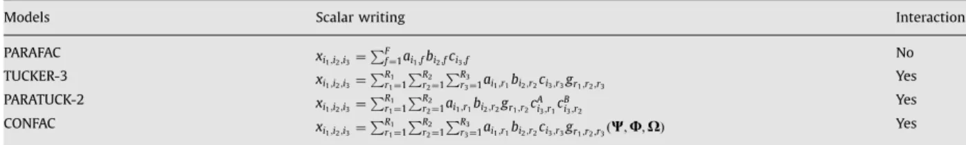
Table 1 summarizes the different tensor models in scalar form. The presence of interactions between matrix factors is also indicated. We remark that these interac-tions are, in general, unconstrained in the TUCKER-3 model (a total of R1R2R3 interactions is possible). For

CONFAC, these interactions are controlled by the three constraint matrices

W

,

U

, and

X

, whereas for PARATUCK-2 the interaction pattern is defined byCAandCB.

In the next section, we exploit the constrained PARATUCK-2 model to design the structure of the multiple-antenna transmission scheme used at the transmitter.

3. Proposed space–time spreading–multiplexing model

data streams composed ofNsymbols each. The proposed space–time spreading–multiplexing model consists in jointly multiplexing/allocating the Rdata streams across

space and time dimensions, i.e. across M transmit antennas andPtime-slots. Each time-slot corresponds to

one channel use (N symbol periods) for transmitting

the data streams. Fig. 2illustrates the proposed space–

time spreading–multiplexing model. The stream-to-slot

allocation block determines the mapping of the R data streams across the P time-slots. Likewise, the antenna-to-slot allocationblock determines the mapping of theM

transmit antennas to thePtime-slots. We call attention to the fact that the same data stream and antenna can be allocated to (i.e. repeated over) more than one time-slot.

Define

m

p2 ½1;Rand

g

p2 ½1;Mas the number of data

streams and transmit antennas allocated to thep-th time-slot, respectively,p¼1;. . ._;P. The spatial precoder com-bines the

m

pdata streams to generate

g

pprecoded streams

which are then transmitted by a subset of

g

p transmit

antennas at the p-th time-slot. After precoding over P

time-slots, the resulting data streams are properly organized at each transmit antenna and then parallel-to-serial converted before being transmitted. The wireless channel is characterized by rich-scattering Rayleigh

flat-fading propagation and is assumed constant during N

symbol periods. The data streams are transmitted with the same power and the total transmitted power is normalized at any channel use and is independent on the number of data streams and transmit antennas.

3.1. Allocation structure

Let us define the stream-to-slot allocation matrix

_W

2

C

PR

and theantenna-to-slot allocation matrix

U

2

C

PM

, which are composed uniquely of 1’s and 0’s. These matrices are known to both the transmitter and the receiver, and constitute the core of the space–time precoder. We have

m

p¼

XR r¼1

c

p;r,

g

p¼

XM m¼1

f

p;m. (12)

Thep-th row

Wp

2

C

1Rof

W

determines which

m

p data

streams are allocated to thep-th slot. Likewise, thep-th row

_U

p2

C

1

M

of

_U

determines which

g

p transmit

antennas are allocated to the p-th slot. For example, suppose that

m

p¼2 and

g

p¼3 with

Wp

¼ ½110 and

U

p¼ ½1011. This means that the first and the second data

streams will be transmitted by the first, third and fourth transmit antennas at thep-th slot. Since each time-slot has its own stream-to-antenna allocation, different levels of space–time multiplexing and diversity are possible by varying the pattern of 1’s and 0’s of

W

and

U

. The allocation matrices satisfy the two following

assumptions:

(A1) Both

W

and

U

have no all-zero row. This means that during each time-slot at least one data stream is

M

···

···

···

···

···

···

···

···

1

Stream-to-slot allocation

Antenna-to-slot allocation 1

Input data streams

Precoded

R

1

µ γ1

P µ

P/S

P/S P P

P γ

{s_1,1 s_N,1}

{s_1,R s_N,R} _(Ψ)

Time-slot 1

Time-slot P

Precoding Precoding

(W)

(W)

(Φ)

symbols Temporally-allocated

symbols transmitted signal

Space-time

Fig. 2.Proposed space–time spreading–multiplexing model as a cascade of three blocks: (i) stream-to-slot allocation, (ii) precoding, and (iii) slot-to-antenna allocation.

Table 1

Main third-order tensor models in scalar form.

Models Scalar writing Interactions

PARAFAC xi1;i2;i3¼PFf¼1ai1;fbi2;fci3;f No TUCKER-3 xi1;i2;i3¼PR1r1¼1

PR2 r2¼1

PR3

r3¼1ai1;r1bi2;r2ci3;r3gr1;r2;r3 Yes PARATUCK-2 xi1;i2;i3¼PR1r1¼1

PR2

r2¼1ai1;r1bi2;r2gr1;r2cAi3;r1cBi3;r2 Yes CONFAC xi1;i2;i3¼

PR1 r1¼1

PR2 r2¼1

PR3

transmitted and at least one transmit antenna is used.

(A2) Both

_W

and

_U

have no all-zero column. This means that every data stream and transmit antenna is allocated at least once during thePtime-slots.

Note that R data streams pass through the channel

duringPtime-slots of durationNsymbol periods. There-fore, the rate of the space–time transmission is given by

Rate¼ R

P log2ð

n

Þbits per channel use, (13)

where

n

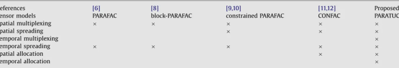
is the modulation cardinality.

Table 2 summarizes the existing tensor-based ap-proaches for space–time transmission in MIMO wireless communication systems. On the top, the reference number is shown along with the used tensor model. Then, the capability to cope with multiplexing and spreading in both space and time domains is indicated. At the bottom of the table, data stream allocation flexibility across transmit antennas (spatial allocation) and time-slots (temporal allocation) is also mentioned.

3.2. Tensor modeling of the received signal

Let us defineS2

C

NRas the symbol matrix collecting the N symbols of theR data streams, where sn;r¼ ½Sn;r

denotes the n-th transmitted symbol of the r-th data stream. The MIMO channel is defined byH2

C

KM, where

hk;m¼ ½Hk;m is the complex coefficient of the channel

associating the m-th transmit antenna with the k-th

receive antenna. Define also the spatial precoding matrix

W2

C

MR

that combinesRdata streams withMtransmit antennas. The structure ofWwill be discussed later. The transmitted space–time signal is given by

um;n;p¼

XR r¼1

wm;rsn;r

f

p;m

c

p;r, (14)

whereum;n;pis the signal transmitted by them-th transmit

antenna at then-th symbol period of thep-th time-slot, i.e. the ðm;n;pÞ-th element of the transmitted signal tensor

U

₂

C

MNP

. In absence of noise, the discrete-time baseband version of the received signal tensor is given by

xk;n;p¼

XM m¼1

hk;mum;n;p

¼ X

M m¼1

XR r¼1

hk;msn;rwm;r

f

p;m

c

p;r, (15)

wherexk;n;pis the received signal associated with thek-th

receive antenna,n-th symbol period andp-th time-slot. It is the ðk;n;pÞ-th element of the received signal tensor

X

2

C

KNP. Note that (15) follows a PARATUCK-2 model, and the correspondences between (7) and (15) are

ðI1;I2;I3;R1;R2Þ2ðK;N;P;M;RÞ

ðA;B;G;CA;CBÞ2ðH;S;W;

U

;

W

Þ. (16)

Let us define Xp2

C

KN as the p-th matrix ‘‘slice’’

obtained by slicing

X

2

C

KNP

along its third dimension. Using (9) and (16), this matrix can be factored as

Xp¼HDpð

U

ÞWDpð

W

ÞST

¼HFpST, (17)

where

Fp¼Dpð

U

ÞWDpð

W

Þ 2

C

MR (18)

is thep-th slice of the overall space–time precoder tensor

F

₂

C

MRP. This slice associates the R data streams to theMtransmit antennas at thep-th time-slot through the precoding matrixW. Note that (17) can alternatively be written in the following form:

Xp¼HUp, (19)

where

Up¼FpST (20)

represents thep-th slice of the transmitted signal tensor

U

2

C

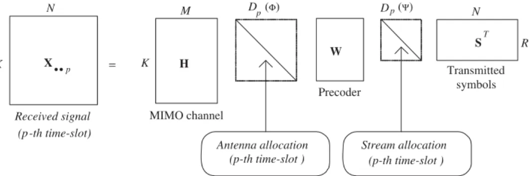
MNP.Fig. 3illustrates the factorization of thep-th sliceXpof the received signal tensor as a function of the

system parameters. Let us define

X1¼ ½vecðX1Þ;. . .;vecðXPÞ 2

C

KNP (21)

as a matrix ‘‘unfolding’’ of the received signal tensor

X

₂

C

KNP, stacking column-wise thePmatrix-slices in vectorized form, each column being associated with a given time-slot. Applying property (2) to (17) gives

X1¼ ðSHÞ½vecðF1Þ;. . .;vecðFPÞ

¼ ðSHÞF1, (22)

where

F1¼ ½vecðF1Þ;. . .;vecðFPÞ

¼diagðvecðWÞÞð

W

T

U

TÞ 2

C

MRP. (23)

Demonstration: Applying property (2) to (18) with

ðA;B;CÞ ! ðDpð

U

Þ;Dpð

W

Þ;WÞ, we obtain

vecðFpÞ ¼ ðDpð

W

Þ Dpð

U

ÞÞvecðWÞ 2

C

RM. (24)

Table 2

Summary of different tensor-based approaches for space–time MIMO systems.

References [6] [8] [9,10] [11,12] Proposed

Tensor models PARAFAC block-PARAFAC constrained PARAFAC CONFAC PARATUCK-2

Spatial multiplexing

Spatial spreading

Temporal multiplexing

Temporal spreading

Spatial allocation

Note that Dpð

W

Þ Dpð

U

Þ 2

C

RMRM is a diagonal matrix

that can be equivalently defined as

Dpð

W

Þ Dpð

U

Þ¼:diagð

W

Tp

U

T pÞ.

Using the fact that diagðaÞb¼diagðbÞa, we can rewrite (24) as

vecðFpÞ ¼diagðvecðWÞÞð

W

Tp

U

T

pÞ. (25)

Concatenating vecðF1Þ;. . .;vecðFPÞ column-wise, and

using definition (1) of the Khatri–Rao product, we get:

F1¼ ½vecðF1Þ;. . .;vecðFPÞ

¼diagðvecðWÞÞ½

W

T1

U

T 1;. . .;

W

T P

U

T P,

¼diagðvecðWÞÞð

W

T

U

TÞ 2

C

MRP

,

which coincides with (23). &

In addition to the matrix unfoldingX1defined in (21),

we can also define two other matrix unfoldings X22

C

PKNandX32

C

PNK from the set of slicesfX1;. . .;XPg,

in the following manner:

X2¼ X1

. . .

XP

2 6 6 6 4 3 7 7 7 5¼

HF1

. . .

HFP

2 6 6 6 4 3 7 7 7 5S T ¼ H ._. . H 2 6 6 4 3 7 7 5 |fflfflfflfflfflfflfflfflfflfflffl{zfflfflfflfflfflfflfflfflfflfflffl} Ptimes

F1

. . .

FP

2 6 6 6 4 3 7 7 7 5S

T_{¼ ð}

IPHÞF2ST (26)

and

X3¼ XT1

. . .

XTP

2 6 6 6 6 4 3 7 7 7 7 5¼

SFT1 . . .

SFTP

2 6 6 6 6 4 3 7 7 7 7 5H T ¼ S ._. . S 2 6 6 4 3 7 7 5 |fflfflfflfflfflfflfflfflfflffl{zfflfflfflfflfflfflfflfflfflffl} Ptimes FT₁

. . .

FTP

2 6 6 6 6 4 3 7 7 7 7 5H T

¼ ðIPSÞF3HT, (27)

where

F2¼ F1

. . .

FP

2 6 6 4 3 7 7 52

C

PMR

and F3¼

FT₁ . . .

FTP

2 6 6 6 4 3 7 7 7 52

C

PRM

(28)

are the two corresponding unfoldings of the precoder tensor constructed from the set of precoder slices

fF1;. . .;FPg.

The factorization of the three matrix unfoldingsX1,X2

and X3 given, respectively, in (22), (26) and (27) is

important for studying the identifiability of the proposed PARACTUCK-2 MIMO system model, which is the subject of Section 5.

4. Design examples

We present some examples of transmission schemes covered by the proposed PARATUCK-2 space–time spreading– multiplexing model. The goal is to show existing relationship between the joint structure of the allocation matrices

W

and

U

and the degree of multiplexing and spreading across

transmit antennas and time-slots. These examples also illustrate the factorization of the space–time precoder in (18) with its associated physical meaning.

Example 1. ðR¼2;M¼3;P¼3Þ: We consider the trans-mission of two data streams using three transmit antennas and three time-slots. The following allocation structure is used:

W

¼ 1 1 1 0 0 1 2 6 4 3 7

5;

U

¼

1 1 1

1 1 0

0 0 1

2 6 4 3 7 5.

Using (18), we have

F1¼W; F2¼

w1;1 0 w2;1 0

0 0 2 6 4 3 7 5; F3¼

0 0

0 0

0 w3;2

2 6 4 3 7 5.

= K H

M MIMO channel K N W T S N R Transmitted symbols Precoder p • • X

Antenna allocation Stream allocation

Received signal (p -th time-slot)

p

D

(Φ) (Ψ) p

D

(p-th time-slot ) (p-th time-slot )

From (20), we obtain the following expressions for the transmitted signal:

U1¼WST; U2¼ w1;1ST1 w2;1ST1 01N

2 6 6 4

3 7 7

5; U3¼ 01N 01N w3;2ST2

2 6 4

3 7 5.

In the first time-slot, all the data streams are jointly spread and multiplexed acrossallthe transmit antennas, representing a full spreading and multiplexing operation. In the second time-slot, the first data stream is trans-mitted using the first and second transmit antennas. This means that no multiplexing takes place in the second time-slot since only a single data stream is transmitted. Moreover, the spatial spreading is only partial since the third transmit antenna is not used. In the third time-slot, only the second data stream is transmitted using the third transmit antenna. In other words, multiplexing and spreading do not take place in the third time-slot, since a single data stream is transmitted using a single transmit antenna.

Example 2. ðR¼3;M¼2;P¼3Þ: Now, we consider the transmission of three data streams using two antennas and three time-slots with the following allocation struc-ture:

W

¼

1 1 1

1 0 1

0 1 1

2 6 4

3 7

5;

U

¼

1 1

1 0

0 1

2 6 4

3 7 5.

We have

F1¼W; F2¼

w1;1 0 w1;3

0 0 0

; F3¼

0 0 0

0 w2;2 w2;3

" #

,

yielding the following transmitted signal allocations:

U1¼WST; U2¼

w1;1ST1þw1;3ST3 01N

" #

,

U3¼

01N w2;2ST2þw2;3ST3

" #

.

As in the first example, a full spreading–multiplexing precoding operation is used in the first time-slot. The second time-slot is characterized by a partial multiplexing operation, where the first and third data streams are combined to be transmitted by the first transmit antenna. Note also that no spatial spreading takes place in the second time-slot, since only the first transmit antenna is used. The multiplexing–spreading structure of the third time-slot is similar to that of the second one, except that partial multiplexing involves the second and third data streams, which are now transmitted by the second transmit antenna. Another observation concerns the temporal spreading of the data streams. Note that the third data stream appears in all the time-slots, while the first and second data streams are only transmitted in two time-slots. Note that this design has a transmission rate of 1 bit per channel use.

Example 3. ðR¼4;M¼2;P¼4Þ: Here, we consider the transmission of four data streams using two antennas and

four time-slots. The allocation structure is given as follows:

W

¼

1 1 1 1

1 1 0 0

0 1 1 0

0 0 1 1

2 6 6 6 4

3 7 7 7

5;

U

¼

1 1

1 1

1 0

0 1

2 6 6 6 4

3 7 7 7 5,

resulting in the following structures for the precoder slices:

F1¼W; F2¼

w1;1 w1;2 0 0 w2;1 w2;2 0 0

" #

,

F3¼

0 w1;2 w1;3 0

0 0 0 0

" #

; F4¼

0 0 0 0

0 0 w2;3 w2;4

" #

.

In this case, the allocations of the transmitted signal are given by

U1¼WST; U2¼

w1;1ST1þw1;2ST2 w2;1ST1þw2;2ST2

2 4

3 5,

U3¼

w1;2ST2þw1;3ST3 01N

" #

; U4¼

01N w2;3ST3þw2;4ST4

" #

.

It can be seen that both spatial multiplexing and spatial spreading take place in the second time-slot, where the first and second data streams are combined and trans-mitted by the two transmit antennas. The third and fourth time-slots use only one transmit antenna for multiplexing different pairs of data streams. For instance, in the third time-slot, the second data stream is combined with the third data stream. The fourth time-slot transmits again the third data stream, but now combined with the fourth data stream at the second transmit antenna.

As can be seen from these examples, several transmit schemes combining multiplexing and spreading in both space and time domains can be designed by varying the pattern of 1’s and 0’s of the two allocation matrices. Such a design flexibility is one of the key features of the PARATUCK-2 tensor modeling approach from the trans-mitter viewpoint. On the other hand, from the receiver viewpoint, the final goal is to perform a blind symbol and channel recovery. Therefore, a fundamental issue remains to be treated which concerns identifiability and unique-ness of the proposed tensor model. These issues are studied in the next section.

5. Identifiability and uniqueness issues

5.1. Identifiability

The identifiability of the underlying PARATUCK-2 model for the received signal is an important issue since we are interested in a blind channel and symbol estima-tion from the received signal tensor only. More specifi-cally, identifiability in the least squares (LS) sense is linked to the recovery ofSandHfromX2andX3, defined in (26)

Theorem 1 (identifiability condition). Suppose thatSand

Hare full column-rank. Uniqueness of the LS solution forS

andHfrom (26) and (27), respectively, requires thatF22

C

PMRandF32

C

PRMbe full column-rank.

Proof. Let us rewrite the two Eqs. (26) and (27) asX2¼ Z2ST and X3¼Z3HT, where Z2¼ ðIPHÞF22

C

PKR and Z3¼ ðIPSÞF32

C

PNM. Uniqueness of the LS solution for SandHrequires thatZ2andZ3be full column-rank. Note

thatðIPHÞandðIPSÞare also full column-rank sinceS

andHare assumed to be full column-rank. Consequently, rankðZ2Þ ¼rankðF2Þand rankðZ3Þ ¼rankðF3Þ, which means

that F2 and F3 must be full column-rank to ensure the

identifiability ofSandH. &

Corollary 1. Since the identifiability ofSandHrequires that F2 andF3be full column-rank,the numberPof time-slots must satisfy the following necessary condition:

P max R

M ; M

R

, (29)

wheredxedenotes the smallest integer number that is greater or equal tox.

This condition imposes a constraint on the numberPof time-slots of the proposed space–time multiplexing– spreading model. It is a useful condition when we are interested in quickly eliminating the space–time sprea-ding–multiplexing configurations that lead to a noniden-tifiable model. Note, however, that F2andF3 depend on

the structure of the allocation matrices

_W

2

C

PR and

U

2

C

PM

, i.e. on their pattern of 1’s and 0’s. They also

depend on the precoder matrix W. This means that the

stream-to-slot and antenna-to-slot allocations as well as the precoder structure must be properly chosen in order to ensure the full-column rank property forF2andF3. In

the following, a design constraint for the allocation matrices

_W

and

_U

and the choice of the precoder matrix

Ware discussed from the identifiability point of view. According to Theorem 1, the identifiability ofSandHin the LS sense requiresF2andF3 defined in (28) to be full

column-rank. First note that bothF2andF3are formed by

a row-wise concatenation of P submatrices, the p-th

submatrix corresponding to the precoder slice Fp,

p¼1;. . ._;P, which is a function ofWand the p-th row of

W

and

U

. In the sequel, we make use of the following property on the rank of block matrices.

Property: Let A2

C

IKJ and A¯2

C

JKI be formed by a row-wise concatenation ofKsubmatricesB1;. . .;BK, with Bk2

C

IJ,k¼1;. . .;K, in the following manner:

A¼

B1 . . .

BK

2 6 6 4

3 7 7 5; A¯ ¼

BT₁ . . .

BTK

2 6 6 6 4

3 7 7 7 5.

We have

Ais full column-rank if at least one of theBk’s is full

column-rank;

A¯ is full column-rank if at least one of theBk’s is full

row-rank;

The property results from the fact that adding rows to a full column-rank matrix does not modify the rank.

Theorem 2 (sufficient condition). Suppose thatS,Hare full column-rank andWis a nonsingular matrix,which implies M¼Rso that condition(29)is always satisfied.ThenSand

H are identifiable in the LS sense from (26) and (27) if

W1

¼

U1

¼1TM.

Proof. Note that

_W1

¼

U1

¼1TM implies that the first

precoder slice F1 is equal to W. Provided that W is

nonsingular, we can apply the previous property with the correspondencesðA;A¯;I;J;KÞ2ðF2;F3;M;R;PÞ, to conclude

thatF2andF3are both full column-rank. This implies the

identifiability ofSandH, respectively. &

Remark. From the design constraint of Theorem 2 we have the following corollary. WhenMaR, if

W1

¼1

T Rand

U1

¼1TM, then (i)Sis identifiable ifWis full column-rank

and (ii)His identifiable ifWis full row-rank. Otherwise

stated, when W is full column-rank, Theorem 2 only

guarantees the identifiability of S. Nothing can be said about the identifiability ofHin this case. This comes from the fact that rankðF3Þis dependent on thejointpattern of

1’s and 0’s of the allocation matrices

W

and

U

. The same reasoning can be applied whenWis full row-rank.

5.2. Structure ofW

It remains to choose a proper structure for the precoder matrixWso that (i) it is a full rank matrix and (ii) it contains no zeros. This ensures identifiability ofS

and/orHaccording to our previous results. We chooseW

as the following Vandermonde matrix:

W¼

1 w . . . wðR1Þ

1 w2 _{. . . w}2ðR1Þ .

. .

. . .

. . .

. . .

1 wM . . . wMðR1Þ 2

6 6 6 6 4

3 7 7 7 7 52

CMR

; where w¼ej2p=MR_.

(30)

It is to be noted, however, that this choice forWis not unique and does not imply optimality from a space–time code design viewpoint. Since our primary goal is identifia-bility, an optimized design ofWis beyond the scope of this work and will be the subject of future research.

5.3. Uniqueness

The identifiability ofSandHin the LS sense is related with the recovery ofSand Hup to their column space. This can be seen by rewriting (22) as

X1¼ ðSðU1UÞ HðV1VÞÞF1¼ ðbSHbÞðUVÞF1, (31)

where

S¼bSU; H¼HVb , (32)

andU2

C

RR_andV2

C

MM_{are two nonsingular matrices.}

Otherwise stated,symbol identifiabilitymeans thatSandbS

span the same column space. Likewise,channel identifia-bilitymeans thatHandHbspan the same column space.bS

model. Therefore, it is necessary to eliminate any rotational freedom caused by the presence of the

nonsingular transformation matrices Uand V so thatS

andHcan be recovered without this ambiguity.

Theorem 3 (uniqueness). Suppose that S and H are full column-rank.If

W

T

U

Tis full row-rank,thenU¼

a

IRand V¼ ð1=

a

ÞIM,which implies thatSandHare unique up to a scalar factor, i.e

b

S¼ ð1=

a

ÞS and Hb¼

a

H. (33)

Proof. The proof first consists in studying the rank ofF1

given in (23). Note that

rankðF1Þ ¼rankðdiagðvecðWÞÞð

W

T

U

TÞÞ ¼rankð

W

T

U

TÞ

since Wis a Vandermonde matrix that has no zeros by

construction. According to the following equality

ðSHÞF1¼ ðbSHbÞðUVÞF1,

it follows that if F1, and therefore

W

T

U

T, is full

row-rank, then

ðUVÞF1¼F1 implies UV¼F1Fy1¼IRM. (34)

The proof is completed by observing thatUV¼IRM is

only possible when bothUandVare identity matrices up to scalar factors that compensate each other, i.e.U¼

a

IR

andV¼ ð1=

a

ÞIM. &

Discussion: As

W

T

U

T2

R

RMP

, the condition rankð

W

T

U

TÞ ¼RM of Theorem 3 implies P RM. Although

restrictive in practice, we call attention to the fact that this condition is only sufficient but not necessary for uniqueness. In fact, depending on the chosen

configura-tion for

_W

and

_U

, the pattern of zero and nonzero

elements of F1 may restrict the number of nonzero

elements inUandVso thatðUVÞF1¼F1is satisfied. If

such a restriction implies thatU¼

a

IRandV¼ ð1=

a

ÞIMare

the only solutions to this equation, then S and H are

unique, even when PoRM. For instance, in the design

examples of Section 4 we havePoRM and uniqueness is

guaranteed, as will be shown later in our simulation results. Finding a necessary and sufficient condition on the joint structure of

_W

and

_U

that ensures uniqueness in the casePoRMis an open problem.

6. Blind receiver

The proposed blind receiver is based on the well-known alternating least squares algorithm [15]which is the classical solution for estimating the factor matrices of a tensor model in an iterative way. In our case, the ALS algorithm consists in fitting a PARATUCK-2 model to the received signal tensor represented by means of its matrix unfoldings (26) and (27) to jointly estimate the symbol and channel matrices in the presence of an additive white Gaussian noise. Define_X~

j¼XjþVj,j¼2;3, as the noisy

versions of Xj, where Vj is an additive complex-valued

white Gaussian noise matrix. Recall that F2 and F3 are

known since they only depend on the precoder matrixW

and the two allocation matrices

W

and

U

which are

known at both the transmitter and the receiver sides. The

algorithm consists in alternating between the estimation of the channel and symbol matrices in the LS sense, by minimizing the two following conditional criteria:

b

SðiÞ¼arg min S

kX~2 ðIPHbði1ÞÞF2STk2F,

b

HðiÞ¼arg min H

kX~3 ðIPbSðiÞÞF3HTk2F,

where i and k kF denote the iteration number and the

Frobenius norm, respectively. The blind receiver algorithm therefore consists of the following steps:

Initialization: Seti¼0; randomly initializeHbð0Þ; Alternating LS updates:

(1) i¼iþ1;

(2) From_X~

2, calculate an LS estimate ofS:

b

ST_ðiÞ¼ ½ðIPHbði1ÞÞF2yX~2;

(3) FromX~3, calculate an LS estimate ofH:

b

HT_ðiÞ¼ ½ðIPbSðiÞÞF3yX~3;

(4) Repeat steps (1)–(3) until convergence.

We decide the convergence of the algorithm when the error between the received signal tensor and its recon-structed version from the estimated channel and symbol matrices does not significantly change between two successive iterationsiand iþ1. More specifically, let us define

eðiÞ ¼ kX~2 ðIPHbðiÞÞF2bSðiÞkF (35)

as the model estimation error calculated at the i-th

iteration of the algorithm. If

jeðiþ1Þ eðiÞj 106_,

we assume that the ALS algorithm has converged at thei -th iteration. In general, -the ALS algori-thm is sensitive to the initialization and convergence to the global minimum can be slow when all of the matrix factors of the model are unknown. In our case, however, the convergence to the global minimum is almost always achieved regardless of the initialization, since three (of five) matrix factorsW,

W

and

U

of the PARATUCK-2 tensor model are known.

7. Simulation results

value given by

SNR¼10 log₁₀kX1k

2 F

kV1k2F

.

In all cases, we consider a very short data stream ofN¼

10 symbols, which is a challenging assumption for a blind receiver. All the simulations involve the three transmis-sion schemes associated with the design examples described in Section 4.

Recall that the estimation of the symbol and channel matrices are affected by a scaling factor, i.e. bS¼

a

Sand

b

H¼ ð1=

a

ÞH. In order to eliminate this ambiguity, it is enough to know one entry ofS. Here, we assume that the first symbol of the first data stream is equal to 1. In this case, we have ^_s1

;1¼

a

and unambiguous estimates ofS

andHcan be found.

7.1. Convergence of the ALS receiver

We first evaluate the convergence of the ALS algorithm. The results depicted inFig. 4represent the average value of the error between the data tensor and the one reconstructed from the estimated Sand Has a function of the number of iterations. Note that, at each run, this error is calculated from (35) at each iteration. We consider two SNR values and schemes 1 and 2 are simulated. We can observe that scheme 1 presents a lower average estimation error than scheme 2 at the same SNR value. We attribute such a gap to the fact that scheme 1 is more diversity-oriented (fewer data streams than transmit antennas) whereas scheme 2 is more multiplexing-oriented (more data streams than transmit antennas). Consequently, scheme 1 has more spatial degrees of freedom at the transmitter than scheme 2, which leads to a better estimation of the model parameters. We can also see that the impact of the SNR is more significant in scheme 1 than in scheme 2.

In the next experiment, we consider scheme 1 with

K¼2 and 3 receive antennas. The goal is to evaluate the distribution of the required number of runs for achieving the convergence of the ALS algorithm, for several Monte Carlo runs. The results are shown inFig. 5. The maximum

number of iterations allowed for the ALS algorithm is equal to 5000. The histogram is composed of 100 points, each one representing an interval of 50 iterations. It can be seen that the increase in the number of receive antennas yields a better performance in terms of con-vergence speed. Note that forK¼3, the convergence is achieved within 1000 iterations for almost all the runs.

For K¼2, there is a significant number of runs that

require more than 1000 iterations for convergence. These observations corroborate the importance of the spatial diversity at the receiver for improving the receiver performance.

7.2. BER performance

In this section we evaluate the BER performance of two different transmission schemes with the blind ALS receiver. We consider schemes 1 and 2 usingK¼2 or 3 withP¼3. We have also simulated scheme 2 withP¼6, where

W

and

U

in Example 1 of Section 4 are replaced by

¯

W

¼12

W

and

U

¯ ¼12

U

, respectively. The results are

depicted in Fig. 6. First, we can see that scheme 1

0 500 1000 1500 2000 2500 3000 3500 4000 4500 5000 10−4

10−3 10−2 10−1 100

Number of iterations

Average error

scheme 1, SNR=10dB scheme 1, SNR=20dB scheme 2, SNR=10dB scheme 2, SNR=20dB

Fig. 4.Average reconstruction errorversusthe number of iterations.

0 1000 2000 3000 4000 5000 100

101 102 103

Number of iterations for convergence

Number of runs

gray circles: K=2 black cross: K=3 Scheme 1 (R=2, M=3)

Fig. 5.Distribution of the required number of iterations for convergence.

0 3 6 9 12 15 18 21 24 10−5

10−4 10−3 10−2 10−1 100

SNR (dB)

BER

Scheme 1 (R=2, M=3)

Scheme 2 (R=3, M=2)

K=3, P=3

K=3, P=6

K=2, P=3

K=3, P=3

K=2, P=3

outperforms scheme 2. Such a gain comes from the fact that scheme 1 transmits the first data stream over transmit antennas 1 and 2 in the second time-slot, thus providing a higher transmit spatial diversity gain than scheme 2, where no spatial spreading takes place in the second time-slot (c.f. Section 4).

It is worth mentioning, however, that scheme 1 has a lower spectral efficiency than scheme 2. According to (13), the transmission rate of schemes 1 and 2 are, respectively,

equal to 4/3 and 2 (bits per channel use). When P¼6

time-slots are used for scheme 2, the performance is improved at the cost of a reduction of the transmission rate by a factor of two. For instance, an SNR gain of 3 dB is obtained for a BER of 102_{, when the number of time-slots}

is increased from 3 to 6. For both schemes, a performance gain is obtained when the number of receive antennas is increased from 2 to 3, which is an expected result.

7.3. Comparison with the zero forcing (ZF) receiver

In order to provide a performance reference of the proposed PARATUCK-2 MIMO transceiver, we have plotted the performance of the nonblind zero forcing receiver. Contrarily to the proposed transceiver, the nonblind ZF one assumes perfect knowledge of the channel matrix. Using our notation, the ZF receiver consists in a single-step estimation of the symbol matrix given by

b

STZF¼ ½ðIPHÞF2yX~2,

where H is perfectly known. In this comparison, we

consider scheme 1 withK¼2. It can be seen fromFig. 7

that the gap between ALS and ZF is around 5 dB in terms of SNR, for a BER equal to 102_{. We can observe that the}

same performance improvement is obtained for both ZF and ALS when the SNR is increased.

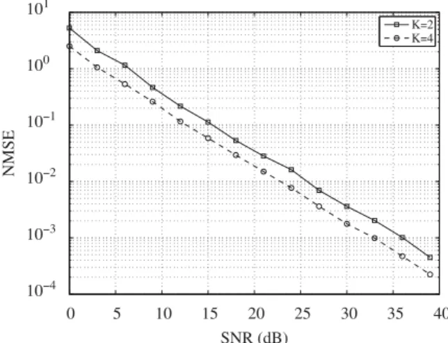
7.4. Channel estimation performance

Although the final goal of the blind receiver is to recover the transmitted information, a blind channel estimation is also afforded by the proposed receiver,

thanks to the uniqueness property of the PARATUCK-2 tensor model. We evaluate the accuracy of the blind channel estimation from the normalized mean square error (NMSE) measure averaged over 1000 Monte Carlo runs and defined as follows:

NMSEðHÞ ¼ 1

1000

X

1000

t¼1

kHbðtÞ Hk2F

kHk2F

,

where HbðtÞ is the channel matrix estimated at conver-gence of the t-th run. In this experiment, we consider Scheme 1 of Section 4.Fig. 8displays the results. Note the linear decrease in the channel estimation error as a function of the SNR. We can also observe that usingK¼4 receive antennas provides an SNR gain of about 3 dB over a

system withK¼2 antennas for any fixed NMSE value.

7.5. Comparison with competing tensor-based MIMO transceivers

Now, the BER performance of the proposed PARATUCK-2 MIMO transceiver is compared with those of competing tensor-based transceivers which rely on other tensor models such as PARAFAC and CONFAC. For this compar-ison, we have selected the Khatri–Rao space–time coding

model of Sidiropoulos and Budampati [6] and the

CONFAC-MIMO coding model of de Almeida et al.

[11,12]. We recall that the KRST coding model consists in transmitting a single data stream per transmit antenna while spreading each data stream in the time domain only. The CONFAC-MIMO coding model additionally exploits the spatial dimension to allocate the data streams to the transmit antennas in different manners. Both the KRST and the CONFAC transceivers use the ALS algorithm to jointly and blindly estimate the channel and symbol matrices. For a fair comparison, the same random initialization is used for all tensor-based transceivers at each Monte Carlo run, and the number of receive antennas and symbol blocks are, respectively, fixed to K¼2 and

N¼10. 0 3 6 9 12 15 18 21 24

10−5 10−4 10−3 10−2 10−1 100

SNR (dB)

BER

ALS ZF

Fig. 7.ALS (blind)versusZF (perfect channel knowledge).

0 5 10 15 20 25 30 35 40 10−4

10−3 10−2 10−1 100 101

SNR (dB)

NMSE

K=2 K=4

For the PARATUCK-2 transceiver, we consider the following space–time spreading scheme:

Wparatuck

2¼

1 1

1 0

0 1

2 6 4

3 7

5;

Uparatuck

2¼

1 1 0

1 0 1

0 1 1

2 6 4

3 7 5.

For the CONFAC transceiver, we consider a transmit scheme characterized by the following allocation ma-trices:

Wconfac

¼

Uconfac

¼ 1 1 0 0

0 0 1 1

" #

,

Xconfac

¼

1 0 1 0

0 1 0 0

0 0 0 1

2 6 6 4

3 7 7 5.

Note that, for the KRST transceiver, only time-domain spreading exists and the allocation matrices are reduced to identity matrices, i.e.

Wkrst

¼

Ukrst

¼

Xkrst

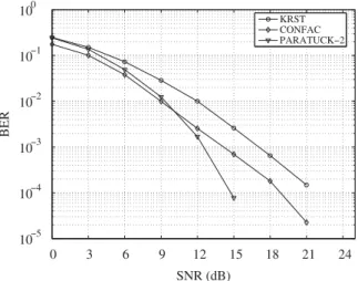
¼I3. For all

transceivers, we have fixed the number of transmit antennas toM¼3 and the number of time-slots toP¼3. According toFig. 9, the PARATUCK-2 transceiver offers the best results for the chosen configuration, outperform-ing the KRST transceiver as well as the CONFAC one at higher SNR levels. Such a performance gain comes from the increased transmit spatial diversity obtained with the PARATUCK-2 transmit scheme by spreading both data streams across two transmit antennas at each time-slot. However, in the low SNR region the CONFAC transceiver presents a slight improvement over the PARATUCK-2 one, due to a higher coding gain obtained by fully spreading the data streams across all the three time-slots. It is worth

noting that R¼2 for the CONFAC and PARATUCK-2

transceivers, while R¼3 for the KRST transceiver. Since QPSK modulation is used, this results in a rate of 2 bits per channel use for the KRST transceiver and 4/3 bits per channel use for the CONFAC and PARATUCK-2 transcei-vers. These results illustrate the existing performance tradeoffs obtained with the different tensor-based MIMO transceivers.

8. Conclusion

In this paper, we have proposed a new tensor modeling approach to space–time spreading–multiplexing for MIMO wireless communication systems with joint blind channel estimation and symbol detection. The core of the proposed PARATUCK-2 model is composed of a precoding matrix and two allocation matrices that allow to control both the spreading and the multiplexing of the data symbols across multiple transmit antennas and time-slots. The PARATUCK-2 space–time transmission structure has the flexibility to allocate the data streams to time-slots in different ways. Identifiability and uniqueness have been discussed and linked to the design of the allocation matrices. We have also derived a blind ALS receiver based on the PARATUCK-2 tensor structure. Perspectives of this work include an extension of the PARATUCK-2 modeling approach to multicarrier systems with space–time–frequency transmission. The study of alternative receiver algorithms is also a topic for future research.

References

[1] G.J. Foschini, M.J. Gans, On limits of wireless communications when using multiple antennas, Wireless Pers. Commun. 6 (3) (1998) 311–335.

[2] V. Tarokh, N. Seshadri, A.R. Calderbank, Space–time codes for high data rate wireless communications: performance criterion and code construction, IEEE Trans. Inf. Theory 44 (2) (March 1998) 744–765.

[3] S. Mudulodu, A.J. Paulraj, A simple multiplexing scheme for MIMO systems using multiple spreading codes, in: Proceedings of 34th ASILOMAR Conference on Signals, Systems and Computers, Pacific Grove, USA, vol. 1, 29 October–1 November, 2000, pp. 769–774. [4] R. Doostnejad, T.J. Lim, E. Sousa, Space–time multiplexing for MIMO

multiuser downlink channels, IEEE Trans. Wireless Commun. 5 (7) (2006) 1726–1734.

[5] M. Vu, A. Paulraj, MIMO wireless linear precoding, IEEE Signal Process. Mag. 24 (5) (Sep. 2007) 86–105.

[6] N.D. Sidiropoulos, R. Budampati, Khatri–Rao space–time codes, IEEE Trans. Signal Process. 50 (10) (2002) 2377–2388.

[7] R.A. Harshman, Foundations of the PARAFAC procedure: model and conditions for an ‘‘explanatory’’ multi-mode factor analysis, UCLA Work. Pap. Phonet. 16 (December 1970) 1–84.

[8] A. de Baynast, L. De Lathauwer, B. Aazhang, Blind PARAFAC receivers for multiple access-multiple antenna systems, in: Proceedings of VTC Fall, Orlando, USA, October 2003.

[9] A.L.F. de Almeida, G. Favier, J.C.M. Mota, Space–time multiplexing codes: a tensor modeling approach, in: Proceedings of IEEE SPAWC, Cannes, France, July 2006.

[10] A.L.F. de Almeida, G. Favier, J.C.M. Mota, Multiuser MIMO system using block space–time spreading and tensor modeling, Signal Process. 88 (6) (October 2008) 2388–2402.

[11] A.L.F. de Almeida, G. Favier, J.C.M. Mota, Constrained tensor modeling approach to blind multiple-antenna CDMA schemes, IEEE Trans. Signal Process. 56 (6) (June 2008) 2417–2428.

[12] A.L.F. de Almeida, G. Favier, J.C.M. Mota, A constrained factor decomposition with application to MIMO antenna systems, IEEE Trans. Signal Process. 56 (6) (June 2008) 2429–2442.

[13] L.R. Tucker, Some mathematical notes on three-mode factor analysis, Psychometrika 31 (1966) 279–311.

[14] R.A. Harshman, M.E. Lundy, Uniqueness proof for a family of models sharing features of Tucker’s three-mode factor analysis and PARAFAC/CANDECOMP, Psychometrika 61 (1) (March 1966) 133–154.

[15] R. Bro, Multi-way analysis in the food industry: models, algorithms and applications, Ph.D. Dissertation, University of Amsterdam, Denmark, 1998.

[16] A. Kibangou, G. Favier, Blind joint identification and equalization of Wiener–Hammerstein communication channels using PARATUCK-2

0 3 6 9 12 15 18 21 24 10−5

10−4 10−3 10−2 10−1 100

SNR (dB)

BER

KRST CONFAC PARATUCK−2

tensor decomposition, in: Proceedings of EUSIPCO, Poznan, Poland, September 2007.

[17] H.A. Kiers, J.M.F. ten Berge, R. Rocci, Uniqueness of three-mode factor models with sparse cores: the 333 case, Psychometrika 62 (3) (1997) 349–374.

[18] H.A. Kiers, A.K. Smilde, Constrained three-mode factor analysis as a tool for parameter estimation with second-order instrumental data, J. Chemometr. 12 (2) (December 1998) 125–147.

[19] J.M.F. ten Berge, A.K. Smilde, Non-triviality and identification of a constrained Tucker3 analysis, J. Chemometr. 16 (2002) 609–612. [20] J.M.F. ten Berge, Simplicity and typical rank of three-way arrays,

with applications to Tucker3 analysis with simple cores, J. Chemometr. 18 (2004) 17–21.