The accuracy of the escrowed dividend model on the value of European options on a stock paying discrete dividend

A Work Project, presented as part of the requirements for the Award of a

Master Degree in Finance from the NOVA - School of Business and

Economics.

Directed Research

The accuracy of the escrowed dividend model on the value of

European options on a stock paying discrete dividend

Weiqing Wu

Student Number: 769

A Project carried out on the finance course, under the supervision of:

Prof. João Amaro de Matos

Abstract

This project characterizes the accuracy of the escrowed dividend model on the value of European options on a stock paying discrete dividend. A description of the escrowed dividend model is provided, and a comparison between this model and the benchmark model is realized. It is concluded that options on stocks with either low volatility, low dividend yield, low ex-dividend to maturity ratio or that are deep in or out of the money are reasonably priced with the escrowed dividend model.

Table of Contents

 Intuitions of the results ... 13

References... 19

Introduction

The aim of this project is to characterize the accuracy of the escrowed dividend model. This model has been widely used to approximate the value of European options written on stocks paying discrete dividend. Although the model has been popular amongst practitioners, its accuracy has not been properly discussed.

Derivatives play a very important role in the finance market. In particular, options are actively traded by financial institutions, or fund managers in the over-the counter market for hedging or speculation. Choosing the most appropriate pricing method is critical for option traders to succeed.

Many option pricing models have been developed to value options. However, depending on the nature of each option, different valuation methods should be applied. For example, to value European options without dividend payment, the Black-Scholes (BS) model (1973) gives the correct value under the Black-Scholes context. Variants of the BS model have been developed to deal with options with different properties. But for European options with discrete dividend payment, apart from numerical models such as the Monte Carlo option model, it has had no exact mathematical representation for a long period of time.

Although the escrowed dividend model has been commonly used to price European options with discrete dividend, it does not provide exact valuation. Valuation of options written on an underlying asset that pays a discrete dividend is relatively complex. Fortunately, an integral representation (Amaro de Matos, Dilão and Ferreira 2009) under the Black-Scholes assumptions was found to provide the exact value for

European options written on stock paying discrete dividend. This model has been used as the benchmark for pricing European options on discrete dividend-paying stocks.

Due to the application and popularity of the escrowed dividend model, it is important to understand the general performance of the model. By comparing this model to the benchmark model, we characterize the range of parameters in which the approximation model works, providing results regarding the accuracy of the escrowed dividend model under the Black-Scholes assumptions.

Literature Review

In 1973, Black and Scholes presented a solution to the problem of European option valuation. The Black-Sholes formula is still popular in the financial world. Besides the assumption that the stock price follows a geometric Brownian motion, the absence of any discrete dividend is also a key for the validity of the closed form. Nonetheless, many underlying assets distribute dividends, a fact that violates the Black Scholes assumptions.

Merton extended the application of Black Scholes´s differential equation to options that pay continuous dividend yield or discrete dividend proportional to the stock price in the same year. However, assuming a continuous dividend rate for options on a single stock is usually unrealistic. So if the dividend payment during the option life is discrete, the extended formula is no longer suitable.

Black (1975) was the first to propose an approach to estimate a European option written on a risky stock paying a single dividend, although indirectly, known as the escrowed dividend approach. The basic idea is to adjust the current stock price by

deducting the present value of future dividends, and the actual stock price is replaced in the BS formula.

Many adjustments to the volatility have been studied. Chriss (1997) suggested a simple adjustment that increases the volatility relative to the escrowed dividend process. Unfortunately, the volatility is excessively increased if the dividend is paid out early in the option´s lifetime, which generally overprices call options1.

Beneder and Vorst (2001) proposed another approximation, namely a time-varying weighted average of an adjusted and unadjusted variance. Haug, Haug and Lewis (2003) also made the volatility process more sophisticated by taking into account the timing of the dividend. Unsuccessfully, the authors concluded that this method performs poorly for multiple dividends stock options.

The discrete dividend distribution problem has received a lot of attention, but its complexity also caused confusion. Despite many other different methods tried to solve the problem, none of them were able to present a closed form to value European options with discrete dividend payments. Amaro de Matos, Dilão and Ferreira (2009) proposed a closed-form integral representation and a computational method for the analytical solution of the problem leading to the exact value for such options under the original assumptions of the geometric Brownian motion. Their method is computationally faster than any other exact computational method available, including Monte-Carlo simulations.

Discussion

This chapter is divided into three sections. The first section explains the stochastic price process, the valuation process, the escrowed dividend model and the exact European option with discrete dividend valuation model. The second section compares the performance of the escrowed dividend model with the exact valuation model, allowing to characterize for which parameters’ regions the approximation works well. The last section explains the intuitions behind the results found in section two.

 The model

This section starts by showing the stochastic process of the stock price. Let 𝑆_𝑡 be

the value of a stock at time t, and let T denote the time to maturity of the option on an underlying stock. As mentioned earlier, the stock price follows the geometric Brownian motion. When the underlying asset pays a cash dividend 𝐷 at time 𝜏, a jump of size 𝐷 is

expected:

𝑆_𝑡∗ = {𝑆𝑡− 𝑃𝑉(𝐷), 𝑡 < 𝜏

𝑆𝑡, 𝑡 ≥ 𝜏 ( 1)

where 𝑆_𝑡 represents the risky part of the price process and 𝐷 is the riskless part of the

price. After paying the dividend, no further dividend discount is necessary since only one dividend payment is expected until maturity. Wilmott (2000) stated that if the price jump due to the distribution of dividend is known a priori, no surprise is expected at time τ, implying that the value of the option should not suffer jumps on the ex-date.

A European option’s payoff is the maximum between zero and the difference between the stock price at maturity and the strike price specified initially in the contract. To benefit from the upside payoff of the option, a premium is required. Black and Scholes (1973) introduced a formula to calculate the theoretical price (premium) of a

European option under certain assumptions. Conditions such as no dividend distribution, no commissions, and constant risk-free rate and volatility are included, apart from the lognormal price distribution and efficient markets assumptions. While the original Black Scholes model does not allow for dividend payment, it was extended by Merton (1973) to include continuous dividend payments. However, for options written on a single stock, it is unrealistic to assume such a situation. The model in the next paragraph describes how to adapt the Black Scholes model to European option with discrete dividend payments.

The escrowed dividend approach is a popular model amongst practitioners. It is a simple adjustment to the BS formula, where the stock price is replaced by the stock price minus the present value of expected dividend. Let 𝑆₀ denote the initial stock price, 𝐾 the strike price, 𝑟 the risk free rate of interest, 𝜎 the volatility and 𝑇 the time to

maturity, then the formula to value a European option on a stock with a known cash dividend that is assumed to be paid at time 𝜏 is:

𝑐 = (𝑆0− 𝐷𝑒−𝑟𝜏)𝑁(𝑑1) − 𝐾𝑒−𝑟𝑇𝑁(𝑑2) ( 2 )

where 𝑑1 =

𝐿𝑛(𝑆0−𝐷𝑒−𝑟𝜏_𝐾 )+(𝑟+𝜎2₂)𝑇

𝜎√𝑇 and 𝑑2 = 𝑑1− 𝜎√𝑇.

Despite its simplicity and vast application, it also has few shortcomings. Haug, Haug and Lewis (2003) criticised that the approach often undervalues call options, “Because the stock price is lowered, the approach will typically lead to too little absolute price volatility in the period before the dividend is paid.” Moreover, the authors also argued that “Not only does this yield a poor approximation in certain circumstances, but it can open up arbitrage opportunities!” Such problems have remained until the exact valuation model appeared.

Amaro de Matos, Dilão and Ferreira (2009) presented an integral representation for the value of European options on an asset paying a discrete dividend. The time-zero value of an option written on a stock in such condition is given by:

𝑉(𝑆, 0) = 𝑒−𝑟𝜏 𝜎√2𝜋𝜏∫ 𝑉[𝑆−(𝑦), 𝜏]𝑒𝑥𝑝 [− (𝑥−𝑦)2 2𝜎2_𝜏 ] 𝑑𝑦 +∞ −∞ ( 3 )

where 𝑥 = 𝑙𝑛𝑆 + (𝑟 −𝜎₂2)𝑇 and 𝑆₋ is the value of the stock just before the dividend

payment. Not only is the formula (3) derived, but functional upper and lower bounds for the integral representation are also constructed based on the convexity property of the solutions of the BS equation. These boundary functions are computationally faster and more efficient than any other exact computational method.

 Comparison

In this section, the escrowed dividend approximation result is compared to the exact value for a call option on a stock paying a known discrete dividend at a pre-defined time. Both the escrowed dividend model and the exact valuation model are implemented in the Wolfram Mathematica programme. After running the programme, theoretical prices for the options are obtained and registered for the two models. The accuracy of the escrowed dividend method is measured as the absolute difference between the estimated value and the exact value:

𝜀 = |𝑐 − 𝑉(𝑆, 0)|. ( 4 )

For simplicity, the upper bound of 𝑉(𝑆, 0) is used as the exact value. In the

definition of the relative error, the absolute error should be divided by the true value; since there are situations where the option value may be too small, the use of the

relative error would not be the most adequate choice to describe the accuracy of the escrowed dividend approach.

The numerical example of an option’s parameters is taken from the original paper where the integral representation is obtained. Not only can the correctness of the programme implemented be tested, but the comparison can also be carried out without compromising the goal. The parameters for the upper bound function of 𝑉(𝑆, 0) are: 𝜎 = 0.20, 𝑟 = 0.03, 𝐾 = 100, 𝐷 = 5, 𝑇 = 1 and 𝜏 = 0.5 . In all examples, time is measured in years, 𝜎 and 𝑟 are expressed in annualized terms.

The numerical approaches to partial derivatives are realized for each of the parameters. In practice, each parameter is changed slightly while all the others remain constant. All figures are presented in the appendix.

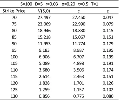
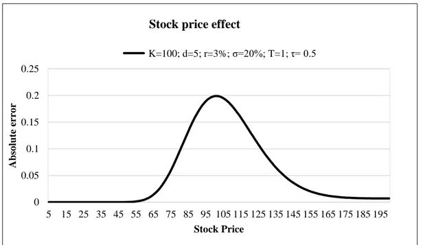
We start by changing the stock price slightly while all the other variables are kept constant. In Figure 1, we compare the results for options with different underlying prices. One of the results is obtained by calculating the upper limit of the numerical integration, using the formula (3), and the other is from the escrowed dividend approach, using the formula (2). The figure shows that the approximated value deviates more from the exact value when the option is at the money, and the error decreases as the stock price moves away from the strike price. Similarly, in Table 1(next page), where the error for the option with different strike prices is presented, we can see that the error has its peak around the point 𝐾 = 100, that is, when the option is at the money.

As a second approach we analyse, what happens to the option value by changing the interest rate, all other parameters being kept constant and the error of the escrowed dividend approach decreases as the interest rate increases. Thus, the value estimated by

the escrowed dividend approach converges to the true value when the interest rate is high (See Figure2).

Table 1: Strike price effect: the difference between the exact value “V(S,0)” and the escrowed dividend approximation “c”, when changing the strike price and keeping all the remaining variables constant.

After conducting more comparisons, more interesting results were obtained. We noticed that, on the one hand, extending the time to maturity of the option would make the escrowed dividend estimate come closer to the true value. On the other hand, delaying the ex-dividend date would make the approximation approach diverge from the exact value. Thus, one can conclude that the earlier the dividend payment and the longer the option maturity, the better the approximation.

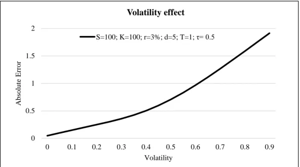
With respect to the volatility, Figure 3 shows that the error increases along with the variable. Thus, options with low volatility are better valued by the approximation than options with high volatility. To conclude the comparison process when changing only one variable, the amount of dividend expected to be paid is studied. It is clear from Figure 4 that options written on stocks that pay a larger cash dividend are priced less

Strike Price V(S,0) c ε 70 27.497 27.450 0.047 75 23.069 22.990 0.079 80 18.946 18.830 0.115 85 15.218 15.067 0.151 90 11.953 11.774 0.179 95 9.183 8.987 0.195 100 6.906 6.707 0.199 105 5.089 4.898 0.191 110 3.680 3.506 0.174 115 2.614 2.463 0.151 120 1.828 1.701 0.126 125 1.259 1.157 0.102 130 0.856 0.775 0.080 S=100 D=5 r=0.03 σ=0.20 τ=0.5 T=1

accurately than options written on stock that pays a small dividend amount, all other variables constant.

In order to better understand how the escrowed dividend model approaches the true option value, a new set of more intuitive variables is considered. Further analysis was carried out on variables such as: the moneyness _𝐾𝑆 , the ex-dividend date to time to

maturity ratio 𝜏

𝑇 , the discrete dividend yield 𝐷

𝑆 , and the volatility. The interest rate is not considered directly in the analysis as its effect is fully embedded in the moneyness variable, since the interest rate enters the BS formula inversely to the strike price, discounting the present value of the strike price.

For any fixed moneyness, options with low 𝜏

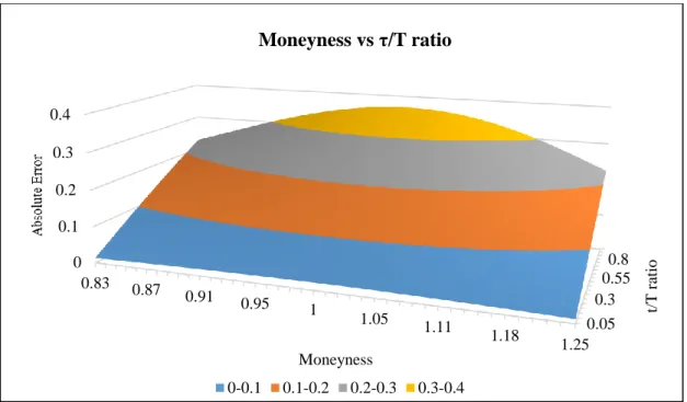
𝑇 ratio, low volatility and low dividend yield are reasonably well priced through the escrowed dividend approximation. Figure 5 shows the error induced when varying only the option´s moneyness and _𝑇𝜏 ratio.

It shows that options with higher _𝑇𝜏 ratios are worse priced by the escrowed dividend

model. Also as mentioned earlier, options near to the money are the ones that suffer more deviation from its fair value when all the other variables are constant. This tendency is maintained even more if the ex-dividend date is set to be at the medium or end of life of the option.

Figure 6 demonstrates the difference in the value of the option by changing merely the moneyness and the volatility level. It shows that options with higher volatility are less precisely estimated by the escrowed dividend model, and that any moneyness change has little if any impact on the valuation process when the stock price variability is high.Figure 7 shows the performance of the approximation when changing only the moneyness and the dividend yield. When the dividend yield does not exist, the

fair value of the option is correctly estimated by the approximation. As the dividend yield raises and the option gets more in the money, the divergence gets more significant. In Figure 8, when the volatility and the dividend yield are changed, the option’s value is also differently estimated. If the volatility and the dividend yield are increased at the same time, the error is also increased. However, when the dividend yield is small, the error induced by increasing the volatility is much lower than it would be if the dividend yield were large (see Figure 9). Analogously, by changing the ex-dividend date to maturity ratio with the dividend yield, keeping all the other variables constant, one can conclude that the value of an option written on a stock that pays higher and later dividend has a larger error. In addition, the higher the dividend, the larger the error induced by delaying the dividend distribution (see Figure 10).

For the example used in the comparison, the maximum error when changing the stock price or the interest rate is 0.20 units of currency. The same magnitude of error can be achieved either by setting the volatility equal to 0.02, or by setting the cash dividend equal to 5 units of currency, ceteris paribus.

All in all, options under low volatility, low dividend yield, low ex-dividend to maturity ratio and not near the money conditions are priced with relative accuracy with the escrowed dividend model. In other words, it should be acceptable to use the escrowed dividend model if these conditions are met.

 Intuitions of the results

Possible reasons for the findings are discussed in this section. We concluded that options near the money are not adequately priced by the escrowed dividend approximation. As the difference between the stock price and the strike price increases, the mispricing decreases. Moreover, options on a stock with lower volatility are better

estimated by the escrowed dividend approximation than options on stock with higher volatility. All this leads to suggest the following:

The less uncertain the option’s exercise is, the less the escrowed dividend approximation deviates from the exact valuation and the smaller the error is.

When the stock price is significantly in the money, the probability of exercising the option written on such underlying asset is close to one and the error goes to zero. Analogously, when the stock price is considerably out of the money, the probability of exercising one such an option goes to zero and the error also tends to be negligible. In both circumstances, the option valuation is more deterministic. In contrast, if the stock price is close to the strike price, the uncertainty about exercising the option is very large2, leading to a larger error.

Another parameter that can lower the randomness underlying the valuation is the volatility. In the extreme case, when the volatility tends to zero, the only factor that affects the stock price evolution is the interest rate, making the option valuation deterministic.

Graph 1 in the next page shows the price evolution of a stock under two distinct situations. In the first situation (blue line), there is no dividend payment. But in the other situation, dividend payment is assumed at an intermediate time, implying a jump of size D in the stock value to the red line. The stock has its price level of 𝑆₀ at time

zero; in the absence of volatility and dividend payment, the stock price at maturity increases only by the interest rate 𝑟 to 𝑆_𝑇 = 𝑆₀𝑒𝑟𝑇_{. Likewise, in the case where the} dividend is considered at time τ, the stock price at that point of time would be 𝑆_𝜏 =

2 _{The probability in such situation lied on the middle range, it is hard to say whereas the option would end}

𝑆₀𝑒𝑟𝜏 _{− 𝐷 right after the dividend payment. At maturity this stock would have} incorporated more time value and it would be valued at 𝑆′

𝑇 = 𝑆𝜏𝑒𝑟(𝑇−𝜏).

We now calculate the initial stock price under no dividend and zero volatility consistent with 𝑆′

𝑇 at maturity. By going backwards, the stock would be 𝑆′0 = 𝑆𝜏𝑒−𝑟𝜏 . After doing some maths3, the initial stock value that satisfies the condition is 𝑆′₀=𝑆₀− 𝐷𝑒−𝑟𝜏 _{. Note that this initial value actually assimilates the adjustment of the stock price}

in the escrowed dividend model. Remember that in the approximation model, the underlying asset´s initial price is reduced by the present value of future dividend. That said, the escrowed dividend model should give the exact value for European option paying discrete dividend in the absence of volatility, or in other words, when the option valuation is deterministic.

Another factor that decreases the error as it increases is the interest rate. As mentioned before, the higher the interest rate, the lower the present value of the strike price. In the extreme case when the interest rate tends to infinite, the present value of the

3 _{𝑆′0= 𝑆𝜏𝑒}−𝑟𝜏 _{= [𝑆0}𝑒𝑟𝜏 _{− 𝐷]}𝑒−𝑟𝜏 _{= 𝑆0− 𝐷}𝑒−𝑟𝜏 τ t T 𝑠0 D 𝑠′0 S 𝑠𝜏 𝑠′𝑇 𝑠𝑇

strike price goes to zero, making the call value to approach the stock price4. Hence, the effect of having a high interest rate is similar to the effect of low strike price, but at a smaller rate5. Once the escrowed dividend model works better when the strike price is low, then it should also work with high interest rate.

Besides the moneyness and the volatility, the timing and the value of the dividend payment also affect the estimation of the escrowed dividend model.

The timing and the amount of the dividend paid have an impact on the option valuation. It is assumed that a certain amount of dividend would be paid for sure at a certain point of time 𝜏. Options written on stocks paying a high dividend amount are not

properly priced by the escrowed dividend model. In addition, the error is larger if the dividend is paid later in time. This fact has already been stressed (E. G. Haug 2007).

It is not difficult to understand that when the cash dividend is small, the mispricing is small, since the approximation coincides with the Black-Scholes formula as D tends to zero. Thus, the smaller the dividend announced at time zero, the better the escrowed dividend approximation performs. Regarding the dividend payment time, the impact of paying the dividend at time τ can be smoothed over if the options expiration time is long enough, because the time value of the option is high enough to compensate the deviation caused at the ex-dividend date. That is, after the dividend payment, option is correctly estimated without any dividend distribution. An equivalent way to have the same result is by paying the dividend as early as possible during a fixed time to maturity, reducing uncertainty about the stock level at the time when dividends are paid. Therefore, the lower the ex-dividend date to time to maturity ratio, the better the escrowed dividend approximation results.

4lim

𝑟→∞𝑁(𝑑1) = lim𝑟→∞𝑁(𝑑2) = 1⇒ lim_𝑟→∞ 𝑐 = lim_𝑟→∞[(𝑆0− 𝐷𝑒−𝑟𝜏) − 𝐾𝑒−𝑟𝑇] ⇒ lim_𝑟→∞ 𝑐 = 𝑆0

5_{“However, the same percentage change in the interest rate r-1has a much smaller effect on call values}

Conclusion

We analyse the performance of the escrowed dividend approximation for European options on a stock that pays a dividend 𝐷 at time τ. The objective is to clarify

for what range of the model parameters does the approach provide acceptable results. The larger the difference between the stock price and the strike price of the option, the better the approximation. That is, the option pricing approximation shows better result if the price of underlying asset is significantly deep in the money or deep out of the money. However, if the option is near the money, the escrowed dividend approach may not be the best choice to estimate the option value.

The interest rate change may have an indirect impact on the option valuation through the present value of the strike price. Large interest rates yield better results for the escrowed dividend approximation as compared to low interest rates, all other variables constant.

When the volatility is low, the premium estimated by the escrowed dividend approximation is very close to the exact valuation method. Since the variability of the stock price is low, the option valuation is more a deterministic rather than non- deterministic process.

With respect to the option´s time to maturity, we concluded that the longer the maturity, the more precise the escrowed dividend approximation. Another variable that influences the option pricing formula is the size of the cash dividend. The mispricing is shown to be larger the higher the dividend paid. As the escrowed dividend model reduces the stock price in the beginning of the life of the option by the present value of the dividend, paying a high dividend could reduce also the absolute price variability, which in turn decreases the value of the option, deviating from the exact value. Besides

the size, the dividend timing also influences the performance of the approximation approach. The later the dividend payment the larger the mispricing.

Summing up, options on stocks with either low volatility, low dividend yield, low ex-dividend to maturity ratio or that are deep in or out of the money are reasonably priced with the escrowed dividend model. In other words, it should be acceptable to use the escrowed dividend model if some of these conditions are met.

References

Amaro de Matos, João, Rui Dilão, and Bruno Ferreira. 2009. "On the value of European options on a stock paing a discrete dividend." Jounal of Modelling in

Management 4 (3): 235-248.

Beneder, Reimer, and Ton Vorst. 2001. "Options on Dividends Paying Stocks."

Proceedings of the International Conference on Mathematical Finance.

Shanghai.

Black, Fischer, and Myron Scholes. 1973. "The Pricing of Options and Corporate Liabilities." Journal of Political Economy 81: 637-654.

Black, Fisher. 1975. "Fact and fantasy in the use of options." Financial Analytst Journal 31: 36-72.

C.Cox, Jonh, and Mark Rubinstein. 1985. Options Markets. New Jersey: Prentice-Hall, Inc.

Chriss, Neil A. 1997. Black-Scholes and Beyond: Option Pricing Models. New York: McGraw-Hill.

Frishling, Volf. 2002. "A discrete question." Risk 15: 115-16.

Haug, Espen Gaarder. 2007. The complete guide to Option Pricing Formulas. New York: McGraw-Hill.

Haug, Espen, Jorgen Haug, and Alan Lewis. 2003. "Back to Basics: a new approach to the discrete dividend problem." Wilmott Magazie 37-47.

Merton, Robert C. 1973. "Theory of Rational Option Pricing." The Bell Journal of

Economics and Management Science 4: 141-183.

0 0.05 0.1 0.15 0.2 0.25 5 15 25 35 45 55 65 75 85 95 105 115 125 135 145 155 165 175 185 195 Abs o lute er ro r Stock Price Stock price effect

K=100; d=5; r=3%; σ=20%; T=1; τ= 0.5

Appendices

Figure 1: the performance of the escrowed dividend model when changing the stock price, ceteris paribus.

Figure 2: The performance of the escrowed dividend model on interest rate changes, ceteris paribus.

0 0.05 0.1 0.15 0.2 0.25 r 10% 20% 30% 40% 50% 60% 70% 80% 90% A b so lu te E rr o r Interest Rate

Interest rate effect

0 0.1 0.2 0.3 0.4 0.5 0.6 0.7 0 2 4 6 8 10 12 14 16 18 20 22 24 A b so lu te E rr o r Dividend

Dividend effect

Figure 4: the performance of the escrowed dividend model when changing only the dividend payment, ceteris paribus.

Figure 3: the performance of the escrowed dividend model when changing only the volatility, ceteris paribus.

0.05 0.25 0.45 0.65 0.85 0 0.5 1 1.5 2 2.5 1.18 1.14 1.1 1.06 1.03 1 0.97 0.94 0.92 Vo latilit y Ax is T it le Moneyness Moneyness vs Volatility 0-0.5 0.5-1 1-1.5 1.5-2 2-2.5

Figure 5: the performance of the escrowed dividend model when changing moneyness and ex-dividend date time to the maturity ratio. (σ=0.20, DY=0.05, r=0.03)

Figure 6: the performance of the escrowed dividend model when changing the moneyness and the

volatility. (τ/T = 0.5, DY=0.05, r=0.03) 0.05 0.3 0.55 0.8 0 0.1 0.2 0.3 0.4 1.25 1.18 1.11 1.05 1 0.95 0.91 0.87 0.83 t/T r atio Ax is T it le Moneyness Moneyness vs τ/T ratio 0-0.1 0.1-0.2 0.2-0.3 0.3-0.4

0.05 0.25 0.45 0.65 0.85 0 1 2 3 4 5 6 7 0.01 0.04 _0.07 0.1 _0.13 0.16 _0.19 0.22 _0.25 0.28 Vo latlity Dividend yield

Volatility vs Dividend Yield

0-1 1-2 2-3 3-4 4-5 5-6 6-7 0.01 0.09 0.17 0.25 0 0.2 0.4 0.6 0.8 1 1.2 1.25 1.19 1.14 1.09 1.04 1.00 0.96 0.93 0.89 0.86 0.83 Div id en d y ield Ax is T it le Moneyness

Moneyness vs Dividend Yield

0-0.2 0.2-0.4 0.4-0.6 0.6-0.8 0.8-1 1-1.2

Figure 7: the performance of the escrowed dividend model when changing the moneyness and the

dividend yield. (τ/T= 0.5, σ=0.20, r=0.03)

Figure 8: the performance of the escrowed dividend model when changing the volatlility and the dividend yield. (τ/T= 0.5,S/K=1, r=0.03)

Figure 9: the performance of the escrowed dividend model when changing the dividend yield and the ex-dividend date to maturity ratio. (σ=0.2, S/K=1, r=0.03)

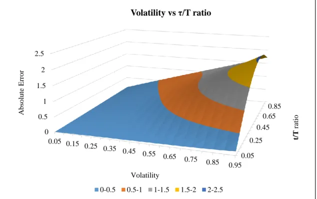
Figure 10: the performance of the escrowed dividend model when changing the volatility and the ex-dividend ratio. (DY=0.05, S/K=1, r=0.03)

0.05 0.25 0.45 0.65 0.85 0 0.2 0.4 0.6 0.8 1 1.2 0.01 0.04 _0.07 0.1 _0.13 0.16 _0.19 0.22 _0.25 0.28 t/T r atio A b so lu te E rr o r Dividend Yield

Dividend Yield vs t/T ratio

0-0.2 0.2-0.4 0.4-0.6 0.6-0.8 0.8-1 1-1.2 0.05 0.25 0.45 0.65 0.85 0 0.5 1 1.5 2 2.5 0.05 0.15 _{0.25 0.35} 0.45 _0.55 0.65 _0.75 0.85 _0.95 t/T r atio A b so lu te E rr o r Volatility Volatility vs τ/T ratio 0-0.5 0.5-1 1-1.5 1.5-2 2-2.5