Sulfur dioxide (SO<sub>2</sub>) as observed by MIPAS/Envisat: temporal development and spatial distribution at 15–45 km altitude

(1)

www.atmos-chem-phys.net/13/10405/2013/ doi:10.5194/acp-13-10405-2013

Atmospheric

Chemistry

and Physics

Sulfur dioxide (SO

2

) as observed by MIPAS/Envisat: temporal

development and spatial distribution at 15–45 km altitude

M. Höpfner1, N. Glatthor1, U. Grabowski1, S. Kellmann1, M. Kiefer1, A. Linden1, J. Orphal1, G. Stiller1, T. von Clarmann1, B. Funke2, and C. D. Boone3

1_{Institute for Meteorology and Climate Research, Karlsruhe Institute of Technology, Karlsruhe, Germany} 2_{Instituto de Astrofísica de Andalucía, CSIC, Granada, Spain}

3_{Department of Chemistry, University of Waterloo, Waterloo, Ontario, Canada}

Correspondence to:M. Höpfner ([email protected])

Received: 29 March 2013 – Published in Atmos. Chem. Phys. Discuss.: 14 May 2013 Revised: 16 August 2013 – Accepted: 19 September 2013 – Published: 29 October 2013

Abstract. We present a climatology of monthly and 10◦

zonal mean profiles of sulfur dioxide (SO2) volume

mix-ing ratios (vmr) derived from MIPAS/Envisat measurements in the altitude range 15–45 km from July 2002 until April 2012. The vertical resolution varies from 3.5–4 km in the lower stratosphere up to 6–10 km at the upper end of the profiles, with estimated total errors of 5–20 pptv for single profiles of SO2. Comparisons with the few available

observa-tions of SO2up to high altitudes from ATMOS for a

volcani-cally perturbed situation from ACE-FTS and, at the lowest altitudes, with stratospheric in situ observations reveal gen-eral consistency of the datasets. The observations are the first empirical confirmation of features of the stratospheric SO₂ distribution, which have only been shown by models up to now: (1) the local maximum of SO₂at around 25–30 km al-titude, which is explained by the conversion of carbonyl sul-fide (COS) as the precursor of the Junge layer; and (2) the downwelling of SO2-rich air to altitudes of 25–30 km at high

latitudes during winter and its subsequent depletion on avail-ability of sunlight. This has been proposed as the reason for the sudden appearance of enhanced concentrations of con-densation nuclei during Arctic and Antarctic spring. Further, the strong increase of SO2to values of 80–100 pptv in the

up-per stratosphere through photolysis of H2SO4has been

con-firmed. Lower stratospheric variability of SO₂could mainly be explained by volcanic activity, and no hints of a strong anthropogenic influence have been found. Regression analy-sis revealed a QBO (quasi-biennial oscillation) signal of the SO₂ time series in the tropics at about 30–35 km, an SAO (semi-annual oscillation) signal at tropical and subtropical

latitudes above 32 km and annual periodics predominantly at high latitudes. Further, the analysis indicates a correla-tion with the solar cycle in the tropics and southern subtrop-ics above 30 km. Significant negative linear trends are found in the tropical lower stratosphere, probably due to reduced tropical volcanic activity and at southern mid-latitudes above 35 km. A positive trend is visible in the lower and middle stratosphere at polar to subtropical southern latitudes.

1 Introduction

Sulfur dioxide (SO2) is one of the key species determining

the aerosol content of the stratosphere (SPARC, 2006). Main sources of stratospheric SO2are the conversion of carbonyl

sulfide (COS) (Crutzen, 1976; Brühl et al., 2012) and the direct transport of SO2 across the tropopause. This

trans-port can occur abruptly through major volcanic eruptions, through upwelling predominantly at the tropical tropopause or through the monsoon circulation (Bourassa et al., 2012). However, there is still a lot of uncertainty regarding the major sources of stratospheric SO₂ during volcanically quiescent periods (Deshler et al., 2006; Hofmann et al., 2009; Vernier et al., 2011; Solomon et al., 2011; Brühl et al., 2012).

Loss of SO₂occurs mainly through oxidation by OH radi-cals into H2SO4vapour, which condenses into liquid sulfate

(2)

a probable further source of SO₂(Rinsland et al., 1995; Vaida et al., 2003; Mills et al., 2005). During winter, downwelling of air in the polar vortices transports elevated amounts of SO₂from the upper stratosphere down to altitudes of 30 km and below. Here, on availability of sunlight in spring, SO₂ is transformed through reaction with OH into H₂SO₄, thus leading to the formation of new particles. These processes have been proposed by Zhao et al. (1995) and Mills et al. (1999, 2005) as an explanation for the sudden formation of enhanced layers of condensation nuclei (CN) in polar spring (Rosen and Hofmann, 1983; Hofmann and Rosen, 1985; Hofmann, 1990; Wilson et al., 1990). However, there has been no direct experimental evidence for this mechanism un-til now.

There exists a large dataset of SO₂ observations from spaceborne nadir-sounding instruments (e.g. Theys et al., 2012, and references therein). While these measurements have a good horizontal resolution, height-resolved profiles cannot be obtained (although some information on plume height has recently been derived: Van Gent et al., 2012; Car-boni et al., 2012). Hence, measurements of the vertical dis-tribution of SO2 in the stratosphere are sparse. This is, for

example, reflected in one of the recommendations within SPARC (2006, p. xii): “Observations of SO2 in the upper

troposphere and lower stratosphere and of H2SO4and SO2

in the middle and upper stratosphere would be extremely valuable to improve our modelling and predictive capabil-ities of stratospheric aerosol.” Under volcanically perturbed situations enhanced mixing ratios of SO2facilitate their

mea-surement. For example, the SO₂ cloud from the eruption of Mt Pinatubo in June 1991 was analysed on the basis of UARS-MLS observations by Read et al. (1993), and ACE-FTS measurements were used to investigate SO₂and sulfate aerosol from the Sarychev eruption in June 2009 (Doeringer et al., 2012).

Only three measured profiles of SO₂covering the altitude range of the stratosphere have been published so far (Rins-land et al., 1995). In their work, on the basis of mean infrared solar occultation spectra during three spaceborne flights of the ATMOS instrument, one SO2 vertical profile per flight

was derived for the altitude range of about 30–50 km. The data revealed high concentrations of SO2in the upper

strato-sphere in the range 100–400 pptv, which was explained by photolysis of H2SO4. However, two of those profiles were

strongly perturbed by the Pinatubo eruption and one possibly, but to a much lesser extent, by El Chichón. Thus, there exists at most one observation of the background stratospheric SO₂ distribution.

In the present work we have analysed infrared limb-emission measurements by MIPAS/Envisat to obtain a global climatology of stratospheric SO2 distributions from July

2002 until April 2012. First attempts at the retrieval of SO2

from MIPAS have previously been performed by Burgess et al. (2005).

After an overview of the instrument (Sect. 2), the retrieval strategy and data characterisation will be described (Sect. 3). Then an overview of the dataset will be given in Sect. 4, fol-lowed by an assessment of its quality through comparison with independent observations and analysis of the internal variability (Sect. 5). In Sect. 6 the distribution of SO₂ will be discussed with respect to the various processes described above, including a regression analysis to single out correla-tions with external parameters, periodic cycles and trends.

2 Instrument

MIPAS (Michelson Interferometer for Passive Atmospheric Sounding) is one of the instruments on ESA’s polar or-biting Envisat satellite (Fischer et al., 2008). Envisat was launched on 1 March 2002, and remained in operation until 8 April 2012, when contact was lost. With one major interrup-tion from April to December 2004, MIPAS measured quasi-continuously from July 2002 until April 2012. The MIPAS FTIR (Fourier transform infrared) limb sounder recorded the radiation emitted by the Earth’s atmosphere in the mid-infrared region with a spectral resolution of 0.025 cm−1

be-fore April 2004 (period 1, P1) and 0.0625 cm−1_{from January}

2005 onwards (period 2, P2). MIPAS was periodically oper-ated in different limb scan patterns. For this work we have used the most frequent “nominal” viewing modes. During P1 these consisted of 17 tangent altitudes (6–68 km with 3 km distances up to 42 km, followed by two steps of 5 km and two steps of 8 km), which do not depend on the geographical po-sition. During P2 the number of tangent views per limb scan was increased to 27. Here tangent altitudes depend on lati-tude ranging from 5–70 km at the poles to 12–77 km over the Equator, with steps increasing with height from 1.5 to 4.5 km. The horizontal distance between two subsequent limb scans in nominal measurement mode was around 550 km during P1 and 420 km during P2, resulting in about 1000 and 1400 limb scans providing full latitudinal coverage per day.

3 Retrieval

Retrieval of SO2 altitude profiles up to the middle

strato-sphere from MIPAS observations is difficult due to its small spectral signal relative to the spectral noise of MIPAS, es-pecially under volcanically non-perturbed conditions. There-fore, we have chosen to analyse monthly mean limb spec-tra binned within 10◦_{-wide latitude bands. This method has}

already been employed for the detection of stratospheric BrONO₂in Höpfner et al. (2009a).

(3)

clouds. We use a CI threshold of 4.5; that is, spectra with CI<4.5 are discarded. Further, all spectra in this limb se-quence are discarded which were measured at lower tan-gent altitudes than those with CI<4.5. Beside thick tropo-spheric clouds, this approach excludes, for example, also cir-rus clouds, polar stratospheric clouds (Höpfner et al., 2009b) and optically thicker aerosol plumes from the subsequent analysis. Depending on atmospheric situation, particle com-position and altitude, the applied CI limit equals a particle volume density of about 1–2 µm3_cm−3_.

In the second step the limb scans that are averaged within each latitude- and time bin are selected. Here we have cho-sen those locations with the lowest available tangent altitude after cloud clearing under the condition that at least 300 limb scans are averaged, which reduced the noise by a factor of at least 17. The noise reduction could be further improved by increasing the required number of samples; this, however, would lead to loss of measurement points particularly at low altitudes and during months with sparser observational cov-erage. A decrease of the required number of samples, on the other hand, would result in larger noise error contribu-tions. For this analysis, MIPAS version 5 level-1b data have been used. Together with the averaged MIPAS spectra, for the retrieval mean, pressure–temperature profiles are calcu-lated from ECMWF analysis data at the position of each sin-gle limb scan. Further, mean tangent altitudes are obtained from the engineering MIPAS tangent altitude values. Errors resulting from these averaging processes are included in the error estimation as described further below.

The retrieval scheme is a constrained global fit approach using all tangent altitudes of one limb scan with averaged spectra simultaneously (e.g. von Clarmann et al., 2003a):

xi+1=xi+

KT_i S−_y1Ki+R

−1

× (1)

h

KT_i S−_y1(ymeas−y(xi))−R(xi−xa)i,

which is a variant of the formulation suggested by Rodgers (2000). Here,xis the vector containing the atmospheric and

instrumental parameters to be determined. The atmospheric profiles are gridded at 1 km altitude levels reaching from 0 to 100 km, in between which the volume mixing ratios (vmr) vary linearly with height.ymeas are the averaged measured

radiances of all tangent altitudes, andSyis the measurement

noise covariance matrix.yi contains the spectral radiances,

which are simulated with the radiative transfer model KO-PRA (Stiller, 2000) using the results obtained in iteration numberi.Ki is the Jacobian matrix, i.e. the partial

deriva-tives∂y(xi)/∂xidetermined in parallel toyiat each iteration

step.x_a contains the a priori profiles. For the target species

SO2, altitude-independent initial guess and a priori profiles, x0 and xa equal 10 pptv, have been used, whereas for all

other trace gases climatological values have been chosen. For the regularisation matrix R a first-order

smooth-ing constraint R=γLTL, where L is a first-order

finite-differences operator (Tikhonov, 1963; Steck, 2002), has been used in order not to bias the retrieval results. Thus, the choice of the constant a priori value for SO₂has no influence on the resulting profiles. The regularisation parameter γ depends only on the species and not on the altitude. It was chosen such to avoid instabilities showing up as oscillations in the retrieved atmospheric profiles.

Line-by-line calculations have been based on the HI-TRAN 2008 compilation including updates until 2010 (Rothman et al., 2009). The spectral intervals (microwin-dows) used for the retrieval are located in the same wavenumber region (∼1366–1377 cm−1_{) within the SO}

2

ν3 band as those selected for the analysis of ACE-FTS

(Doeringer et al., 2012) and of ATMOS data (Rinsland et al., 1995). In detail, we have chosen the four microwin-dows 1366.575–1367.925 cm−1_{, 1369.95–1370.375 cm}−1_,

1371.2–1371.925 cm−1 _{and 1376.0–1376.375 cm}−1 _{in the}

case of the high-spectral resolution mode of MIPAS (P1), and 1366.5625–1367.9375 cm−1_, _{1369.9375–1370.375 cm}−1_,

1371.1875–1371.9375 cm−1 _{and 1376.0–1376.375 cm}−1

for the measurements during P2. These have been selected to gain a good sensitivity for SO2 while avoiding the

strongly interfering spectral signatures of other gases as much as possible. To further minimise these interferences the following gases have been jointly retrieved with SO2:

H2O (isotopologues: H16₂ O, HDO, H18₂ O), CO2, O3, CH4,

HCN and HO2. Further, instrumental parameters that have

been included in the parameter vectorx are a spectral shift

correction per microwindow and an additive calibration off-set per microwindow and tangent altitude. No regularisation has been applied in the case of these instrumental quantities. Figure 1 presents an example of the spectral fit achieved in all four microwindows for MIPAS measurements with higher (top three rows) and lower spectral resolution (bottom three rows). Spectral residuals between measurements and simula-tion are shown for the case where no SO2has been retrieved

(second and fifth row) and under consideration of SO2(third

and sixth row). It is obvious that in both cases, the fit residual is strongly improved by including SO2into the fit parameter

vector, and that the residuals without SO2fit (black lines in

second and fifth row) are mostly produced by SO2spectral

signatures (green lines in second and fifth row).

For characterisation of the vertical resolution of the re-trieval the related averaging kernels have been determined as

A=KTS−_y1K+R

−1

KTS−_y1K. (2)

The rows of A represent the contributions of different

al-titudes to the retrieved vmr profile of SO₂, whereas the columns are the responses of the system to a delta func-tion at the associated altitude. Typical averaging kernels are shown in Fig. 2 for period P1 (top) and P2 (bottom). The overall diagonal structures of A demonstrate that the

(4)

1366.8 1367.2 1367.6 20

40 60 80

Mean spectrum, period: 20021101-20021201, latitude range: 10- 20 deg N, height: 17.3 km

1370.0 1370.1 1370.2 1370.3 20

40 60 80

1371.2 1371.4 1371.6 1371.8 20

40 60 80

1376.0 1376.1 1376.2 1376.3 20

40 60 80 100

1366.8 1367.2 1367.6 -1.5

-1.0 -0.5 0.0 0.5 1.0 1.5

Residuum, black: meas - calc(without SO2), green: calc(with SO2) - calc(without SO2)

1370.0 1370.1 1370.2 1370.3 -1

0 1 2

1371.2 1371.4 1371.6 1371.8 -2

-1 0 1 2

1376.0 1376.1 1376.2 1376.3 -1.0

-0.5 0.0 0.5 1.0 1.5

1366.8 1367.2 1367.6 -1.5

-1.0 -0.5 0.0 0.5 1.0 1.5

Residuum: meas - calc(with SO2)

1370.0 1370.1 1370.2 1370.3 -1

0 1 2

1371.2 1371.4 1371.6 1371.8 -2

-1 0 1 2

1376.0 1376.1 1376.2 1376.3 -1.0

-0.5 0.0 0.5 1.0 1.5

1366.8 1367.2 1367.6 40

60 80 100 120

Mean spectrum, period: 20080901-20081001, latitude range: 50- 60 deg N, height: 15.0 km

1370.0 1370.1 1370.2 1370.3 50

60 70 80 90 100

1371.2 1371.4 1371.6 1371.8 60

80 100 120

1376.0 1376.1 1376.2 1376.3 60

80 100 120

1366.8 1367.2 1367.6 -3

-2 -1 0 1 2

Residuum, black: meas - calc(without SO2), green: calc(with SO2) - calc(without SO2)

1370.0 1370.1 1370.2 1370.3 -2

0 2

1371.2 1371.4 1371.6 1371.8 -4

-2 0 2 4

1376.0 1376.1 1376.2 1376.3 -2

-1 0 1 2 3 4

1366.8 1367.2 1367.6 -3

-2 -1 0 1 2

Residuum: meas - calc(with SO2)

1370.0 1370.1 1370.2 1370.3 -2

0 2

1371.2 1371.4 1371.6 1371.8 -4

-2 0 2 4

1376.0 1376.1 1376.2 1376.3 -2

-1 0 1 2 3 4

Wavenumber [cm-1

]

Radiance [nW/(cm

2 sr cm -1)]

Fig. 1. Spectral identification and fit quality of the SO2retrieval. The columns show the four spectral windows used. The top three rows refer to the first observational period (P1), while rows 4–6 belong to the second period with lower spectral resolution (P2). Rows 1 and 4 contain the measured spectra. The black curves in the panels of row 2 and 5 show the residua after the spectral fit when no SO2is considered, and the black curves in row 3 and 6 are the residua in the case where SO₂is added as a fitting parameter. The green curves in row 2 and 5 indicate the spectral features of SO₂based on simulations only.

lower compared to higher altitudes due to the better sensitiv-ity (higher pressure) and a denser tangent altitude sampling there. Typical values for the vertical resolution as derived from the width of the columns ofAand from the inverse of

the diagonal ofAin both measurement modes vary around

3.5–4 km at 20 km, 4–5 km at 30 km and 6–10 km at 40 km altitude.

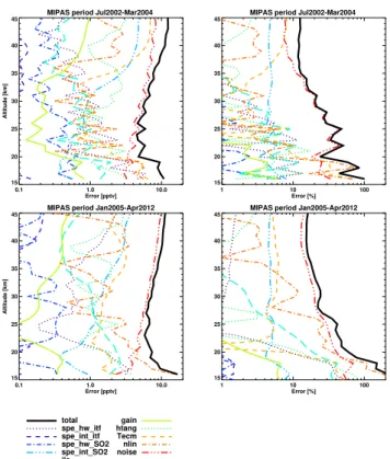
An estimate of the altitude dependent errors is presented in Fig. 3. Typical mean error profiles calculated for one month (January 2003) of period P1 and one month (January 2011) of P2 are shown together with the single error contributions which are combined into the total error by calculating the root sum squared of the single terms.

The following sources of uncertainty have been taken into account: spectroscopic errors of SO2 line intensity

(spe_int_SO2) and air-broadened half-width (spe_hw_SO2). For the line intensity an uncertainty of 5 % has been as-sumed, and for the half width one of 15 %. Both values are on the conservative side of the errors stated in Rothman et al.

(5)

Period: 20030101-20030201, latitude range: 50 - 60 N

15 20 25 30 35 40 45

Altitude [km] 15

20 25 30 35 40 45

Altitude [km]

-0.1

0.0 0.1 0.2 0.3 0.4 0.5 0.6

Period: 20110101-20110201, latitude range: 50 - 60 N

15 20 25 30 35 40 45

20 25 30 35 40 45

Altitude [km]

-0.1

0.0 0.1 0.2 0.3 0.4 0.5 0.6

Fig. 2. Example of averaging kernels for SO₂ at mid-latitudes within the first (top) and the second (bottom) MIPAS measurement period.

These values have been determined from comparison of en-gineering tangent altitude values with those obtained by the pointing retrievals during the standard IMK/IAA data analy-sis (von Clarmann et al., 2003b, 2009; Kiefer et al., 2007).

4 Dataset overview

Figures 4–6 present an overview of all MIPAS results of SO2

as colour-coded cross sections versus time. As mentioned above, the lower altitude limit of the dataset is defined by the condition on the minimum number of limb scans used to cal-culate mean spectra. This is determined by (a) the cloud cov-erage, (b) the scan pattern of MIPAS and (c) the lower limit of 15 km set to confine the retrievals mainly on the strato-spheric situation. The influence of clouds can best be seen at the data gaps during the Antarctic winter season where the MIPAS observations are obscured by polar stratospheric clouds (e.g. top row in Fig. 4). High clouds also restrict some of the observations at low altitudes in tropical regions during P1 until March 2004. Further data gaps covering the whole altitude region are present in 2005 and 2006, when MIPAS

MIPAS period Jul2002-Mar2004

0.1 1.0 10.0

Error [pptv] 15

20 25 30 35 40 45

Altitude [km]

MIPAS period Jul2002-Mar2004

1 10 100

Error [%] 15

20 25 30 35 40 45

MIPAS period Jan2005-Apr2012

0.1 1.0 10.0

Error [pptv] 15

20 25 30 35 40 45

Altitude [km]

MIPAS period Jan2005-Apr2012

1 10 100

Error [%] 15

20 25 30 35 40 45

total spe_hw_itf spe_int_itf spe_hw_SO2 spe_int_SO2 ils

gain htang Tecm nlin noise

Fig. 3.Error estimation of the retrieval for one month during P1 and one month during P2. Considered error sources are the uncertainty of the foreign-broadened half-width and line intensity of interfering species (spe_hw_itf, spe_int_itf), the knowledge of these parame-ters for SO₂(spe_hw_SO2, spe_int_SO2), the uncertainties of the instrumental line shape and gain calibration (ils, gain), the errors in the assumed tangent altitudes and temperatures (htang, Tecm), the error due to the applied technique of retrievals from averaged spec-tra (nlin) and the specspec-tral noise of the instrument (noise). The total error has been determined by quadratic combination of the single error components.

measurements were still sparse during the first years in the new operational mode.

As a basis for subsequent discussions, the dataset has been reduced by averaging to the mean profiles for four seasons (see Fig. 7 and Fig. 8, top two rows). These profiles represent background situations since volcanically strongly perturbed periods, as detailed in the caption of Fig. 7, were neglected during averaging. The related variability is described in the bottom two rows of Fig. 8 by the altitude-dependent standard deviation.

5 Data quality

Here we assess the quality of the MIPAS SO2 dataset by

(6)

15 20 25 30 35 40 45

80

o S - 90 o S

15 20 25 30 35 40 45

70

o S - 80 o S

15 20 25 30 35 40 45

60

o S - 70 o S

15 20 25 30 35 40 45

50

o S - 60 o S

15 20 25 30 35 40 45

o S - 50 o S

Ch

15 20 25 30 35 40 45

30

o S - 40 o S

15 20 25 30 35 40 45

20

o S - 30 o S

15 20 25 30 35 40 45

10

o S - 20 o S

01-Jan

2003 01-Jan2004 01-Jan2005 01-Jan2006 01-Jan2007 01-Jan2008 01-Jan2009 01-Jan2010 01-Jan2011 01-Jan2012

15 20 25 30 35 40 45

0

o - 10 o S

Re Ma Si Ra Me

0 20 40 60 80 100 120 140

vmr [ppt]

<= >=150

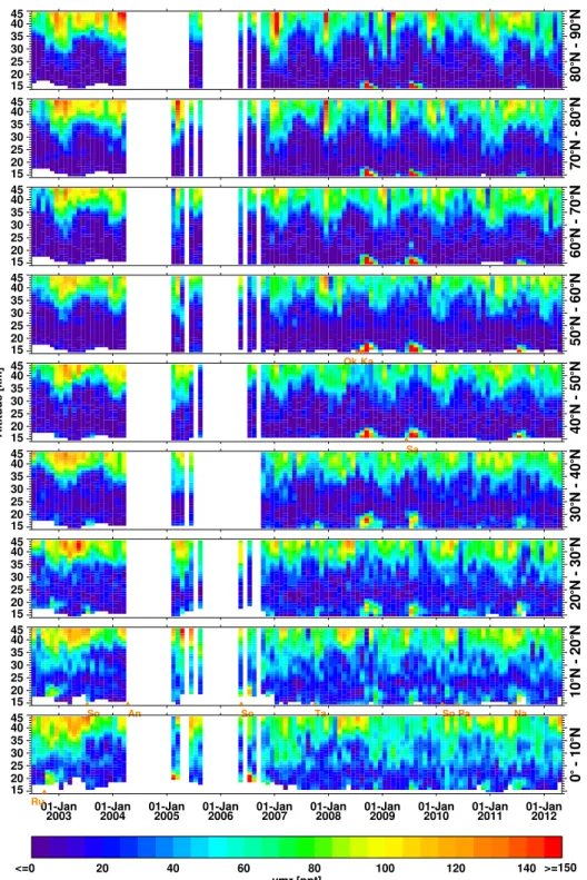
Fig. 4. Time series of colour-coded SO2monthly mean volume mixing ratio profiles for 10◦latitude bins in the Southern Hemisphere. The colour scale is restricted to 0–150 pptv: negative values and those larger than 150 pptv are given the colour corresponding to 0 and 150 pptv, respectively. Major volcanic eruptions are indicated within the latitude bin of their location (see Table 2).

5.1 Comparison with ATMOS

The only measurements of SO2that have reached up to the

upper stratosphere so far were published by Rinsland et al. (1995). These three profiles are compared with MIPAS data

(7)

15 20 25 30 35 40 45

80

o N - 90 o N

15 20 25 30 35 40 45

70

o N - 80 o N

15 20 25 30 35 40 45

60

o N - 70 o N

15 20 25 30 35 40 45

50

o N - 60 o N

Ok Ka

15 20 25 30 35 40 45

o N - 50 o N

Sa

15 20 25 30 35 40 45

30

o N - 40 o N

15 20 25 30 35 40 45

20

o N - 30 o N

15 20 25 30 35 40 45

10

o N - 20 o N

So An So Ta So Pa Na

01-Jan

15 20 25 30 35 40 45

0

o - 10 o N

Ru

0 20 40 60 80 100 120 140

vmr [ppt]

<= >=150

Fig. 5. Same as Fig. 4 but for the Northern Hemisphere.

1985. One should keep in mind that this has also been ob-served under enhanced stratospheric aerosol levels due to the eruption of El Chichón in March 1982, albeit to a lesser extend than ATMOS 1992 and 1993 (SPARC, 2006, e.g. Fig. 4.35).

Throughout the altitude range between 33 and 45 km, the MIPAS mean profile is within the uncertainty range of

AT-MOS 1985. Only at the lowest 2 km MIPAS mean volume mixing ratios of SO2 are about 20 pptv larger than those of

(8)

-50 0 50

h = 16 km

-50 0 50

h = 18 km

-50 0 50

h = 20 km

-50 0 50

h = 22 km

-50 0 50

Latitude [

o]

h = 24 km

Ru Re So An Ma Si SoRa Ta

Ch

Ok Ka Sa

SoPa

Me Na

-50 0 50

h = 27 km

-50 0 50

h = 31 km

-50 0 50

h = 35 km

-50 0 50

h = 40 km

01-Jan

-50 0 50

h = 45 km

0 20 40 60 80 100 120 140

vmr [ppt]

<= >=150

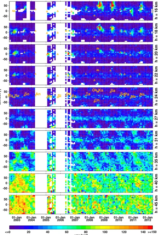
Fig. 6. Global time series of colour-coded SO₂monthly mean distributions at various altitudes. The colour scale is restricted to 0–150 pptv: negative values and those larger than 150 pptv are given the colour corresponding to 0 and 150 pptv, respectively. Major volcanic eruptions are indicated by the latitude of their location (Table 2).

to values of 400 pptv compared to maximum MIPAS values of 100 pptv. The fact that at lower altitudes around 30 km the values of SO2 do not deviate from MIPAS as strongly

as above 35 km, even for volcanically enhanced conditions,

(9)

Table 1.In situ observations of SO2in the lower stratosphere.

Ref. Date Location Altitude VMR

[km] pptv

Jaeschke et al. (1976) Spring 1976 54◦_N ₁₄ ₅₂

Inn and Vedder (1981) Jun–Jul 1979 38, 64, 67◦_N _15.2–20.4 _36–51

Meixner (1984) 1978–80 50◦_N _10.7–15.2 _{Dec: 8–33}

(W-Europe) Apr/May: 13–41(115)

Sep: 25–46

Möhler and Arnold (1992) Feb 1987 67◦_N _tropopause ₁₀₀

(N-Europe) tropopause+2.5 km 10

Thornton et al. (1999) 1991–1996 W-Pacific 12 60

Jurkat et al. (2010) Oct 2008 Europe 11.5 20–55 (strat. background)

510 (Kasatochi)

-50 0 50

Latitude [o_]

15 20 25 30 35 40 45

Altitude [km]

DJF No Volc

0

0 20

20

40 40

40

60 60

60

80

80 vmr [ppt]

0 20 40 60 80 100

-50 0 50

Latitude [o_]

15 20 25 30 35 40 45

Altitude [km]

MAM No Volc

0 0

0

20

40

60 60

60 ₈₀

80

-50 0 50

Latitude [o_]

15 20 25 30 35 40 45

Altitude [km]

JJA No Volc

0 0

0

20

20 20

20

40

60

80

80 80

100

-50 0 50

Latitude [o_]

15 20 25 30 35 40 45

Altitude [km]

SON No Volc

0 0

0

20

20 20

40

60 60

60

80 80

Fig. 7. Mean background seasonal distributions of SO2. Peri-ods of major volcanic influence that have been excluded here are as follows: October–December 2002, July 2003, January– June 2005, May–November 2006, October 2007, July–December 2008, June–December 2009, November–December 2010, July– September 2011.

5.2 Comparison with ACE-FTS

A comparison with observations by ACE-FTS is possi-ble for a volcanically enhanced situation directly after the Sarychev eruption in June 2009. In Fig. 8 of their paper, Doeringer et al. (2012) present the measured zonal median distribution of SO₂between 12 and 20 km for the first half of July 2009. A direct comparison of the ACE-FTS observa-tions (version 3.0) with those of MIPAS is shown in Fig. 10. For the presentation of the ACE-FTS dataset we have (1) calculated the mean, (2) selected the same latitude bands and (3) performed a linear interpolation to the MIPAS al-titude grid. The laal-titude range 30◦_N–40◦_{N cannot be used}

for comparison since there are only two ACE-FTS profiles available, which stem from 1 July and which apparently have not been recorded in volcanically perturbed air masses. Be-tween 40◦_{N and 70}◦_{N, both datasets show the enhanced}

(10)

70o_{N - 90}o_N

1 10 100

VMR [ppt] 15 20 25 30 35 40 45 Altitude [km]

40o_{N - 60}o_N

1 10 100

20o_{N - 40}o_N

1 10 100

0o_{- 20}o_N

1 10 100

VMR [ppt] 15 20 25 30 35 40 45 Altitude [km] DJF MAM JJA SON

70o_{S - 90}o_S

1 10 100

40o_{S - 60}o_S

1 10 100

20o_{S - 40}o_S

1 10 100

0o_{- 20}o_S

1 10 100

VMR [ppt] 15 20 25 30 35 40 45 Altitude [km] JJA SON DJF MAM 70o

N - 90o

N

1 10 100

Stddev(VMR) [ppt] 15 20 25 30 35 40 45 Altitude [km] 40o

N - 60o

N

1 10 100

Stddev(VMR) [ppt] 15 20 25 30 35 40 45 Altitude [km] 20o

N - 40o

N

1 10 100

Stddev(VMR) [ppt] 15 20 25 30 35 40 45 Altitude [km] 0o

- 20o

N

1 10 100

Stddev(VMR) [ppt] 15 20 25 30 35 40 45 Altitude [km]

70o_{S - 90}o_S

1 10 100

40o_{S - 60}o_S

1 10 100

20o_{S - 40}o_S

1 10 100

0o_{- 20}o_S

1 10 100

Fig. 8. Mean background seasonal profiles of SO2(top two rows) and standard deviation of the distribution (bottom two rows). The legend indicating the seasons in the top row refers to the Northern Hemisphere; the legend in the second row is valid for the Southern Hemisphere. The same periods of major volcanic influence as listed in caption of Fig. 7 have been excluded.

5.3 Comparison with in situ observations

In situ measurements of SO₂at comparable altitudes to those presented here for the mean MIPAS profiles are extremely sparse since they have mainly been obtained from aircraft up to the lowermost stratosphere. Table 1 shows a selection of published in situ datasets in which explicitly stratospheric values have been indicated that can best be compared to the mean profiles as shown in Fig. 8. The only in situ dataset reaching into the altitude range presented here is the one ob-tained by Inn and Vedder (1981) up to an altitude of 20.4 km in June/July 1979. The reported values of 36–50 pptv at

15 km are higher (or at the upper end when taking into ac-count the reported error of 50 % of the in situ data) compared to the MIPAS average background vmr distribution (around 13±10 pptv) at mid-latitudes (cf. Fig. 8). At around 20 km, reported SO2 mixing ratios of 45 and 51 pptv (±50 %) at

64 and 67◦_{N are clearly much higher than MIPAS mean}

(11)

0 50 100 150 vmr [ppt] 20 15 10 5 2 Pressure [hPa] ATMOS 1985 30 35 40 45 Altitude [km]

0 100 200 300 400 vmr [ppt] 20 15 10 5 2 Pressure [hPa] ATMOS 1992 30 35 40 45 Altitude [km]

0 50 100 150 200 250 vmr [ppt] 20 15 10 5 2 Pressure [hPa] ATMOS 1993 30 35 40 45 Altitude [km]

Fig. 9. Comparison of MIPAS observations (2003–2012) of SO₂ (red: single; green: mean) with profiles derived from the ATMOS in-strument (black) (Rinsland et al., 1995). Left: SPACELAB 3, April– May 1985, 26◦_N–32◦_{N vs. MIPAS, April–May 20}◦_N–40◦_N.

Middle: ATLAS 1, March–April 1992, 54◦_S–28◦_{N vs. MIPAS,}

March–April 60◦_S–30◦_{N. Right: ATLAS 2, April 1993, 51}◦_S–

44◦_{S vs. MIPAS, April 50}◦_S–40◦_S.

0 20 40 60 80

Latitude [o_]

14 15 16 17 18 19 20 Altitude [km]

July 2009 MIPAS

82 74 61 44 27 659 72 77 76 69 56 39 330 94 122 122 98 63 31 591 94 102 110 102 83 58 501 298 210 122 59 34 1292 417 302 167 75 35 24 1215 419 266 130 32 0 12 1049 416 220 77 8 -9 -2 935 448 210 52 3 0 5 938 vmr [ppt] 0 200 400 600 800 <=

0 20 40 60 80

Latitude [o_]

14 15 16 17 18 19 20 Altitude [km] ACE-FTS 16 11 10 6 7 8 2 502 478 357 219 111 47 32 666 499 333 214 121 61 61 687 502 309 156 66 29 168

Fig. 10. Latitude–height cross section of MIPAS(top) and ACE-FTS (bottom) zonal mean SO₂volume mixing ratios in July 2009. Numbers in white show the exact vmr values of each bin in units of ppt. The available number of profiles used to calculate the zonal means are denoted in orange at the top left of each column.

mean background or the difference points to problems of ei-ther the in situ data or the MIPAS analysis.

Other observations reaching nearly the lower limit of the altitude range of our MIPAS dataset are the first measure-ments of SO2by Jaeschke et al. (1976) at 14 km and

vari-ous stratospheric data by Meixner (1984), both obtained in northern mid-latitudes. Comparing the data in Fig. 8 at the lower end of the profiles with those observations shows that MIPAS mean values are generally at the lower part of the variability of the in situ data. However, when considering the generally increasing MIPAS data at northern mid-latitudes with decreasing altitude, it seems reasonable that the typi-cally higher in situ data at lower heights might be compatible. Since the other stratospheric data listed in Table 1 are similar to those already discussed, we conclude that in general the MIPAS values at the bottom end of their altitude range are at the lower limit of in situ observations.

-50 0 50

Latitude [o

] 15 20 25 30 35 40 45 Altitude [km] 0 1 2 3 4

Fig. 11. Global distribution of1δl,has defined in Eq. (3).

5.4 Internal variability

As described in Sect. 3 the instrument noise dominates the error characteristics over a large part of the profile. We have tried to validate this error term by comparing it to the tem-poral month-to-month variability of the retrieved SO2

pro-files at distinct altitudes for the different latitude bins. This method is similar to the one used for validation of the preci-sion of MIPAS single-scan data products (Piccolo and Dud-hia, 2007). Figure 11 shows for each latitudel and altitude h the standard deviation 1δl,h of the noise-error- (ǫl,h,m)

weighted differenceδl,h,m of the SO2volume mixing ratios

xl,h,mbetween directly subsequent monthsmin time:

1δl,h=

1

M−2

M−1

X

m=1

δl,h,m− ¯δl,h2

!1₂

(3) with

δl,h,m=

xl,h,m−xl,h,m+1

q

ǫ2_l,h,m+ǫ_l,h,m2 ₊₁

, (4)

where M indicates the number of months andǫthe estimated error due to instrument spectral noise. In the ideal case1δl,h

would equal 1. Values greater than 1 indicate either that the natural variability of SO2from month to month is not

neg-ligible (thus increasing the numerator of Eq. 4) or the noise errors are underestimated (denominator of Eq. 4). In Fig. 11, enhanced values of1δl,hin the northern and equatorial lower

stratosphere and at all altitudes in high-latitude regions are very likely due to the natural variability caused by volcanic activity and the downwelling of SO₂-rich air into the po-lar vortices during winter. Anthropogenic influence might be a further source for the enhancements at northern latitudes. Excluding those regions, i.e. for 50◦_S–50◦_{N and altitudes}

≥30 km, the mean value of1δl,h=1.5±0.1. Thus, it can

(12)

6 Results and discussion

6.1 Mid-stratospheric maximum

The main chemical production of SO2in the stratosphere

ap-pears via conversion from COS leading to a local maximum of SO2in the mid-stratosphere (Crutzen, 1976; Brühl et al.,

2012). The MIPAS observations show this maximum to be very pronounced in the tropics, as visible in Figs. 4 and 5, at altitudes of around 27–30 km. The mean latitudinal and seasonal variation of this maximum can better be inspected in averaged stratospheric background profiles as presented in Figs. 7 and 8. For calculation of these profiles major volcani-cally perturbed seasons (for details see caption of Fig. 7) have been excluded. In the tropics, the mid-stratospheric maxi-mum of the mean profiles is located at 28–30 km, decreasing in altitude towards the poles down to 25 km in the northern and 23 km in the southern summer months. In the tropics, the vmr value of the maximum varies at around 40–50 ppt. To-wards higher latitudes, summertime values decrease toTo-wards 20 pptv at subtropics, 10 pptv at middle and 5 pptv at po-lar latitudes. During other seasons the maximum is less dis-cernible from the generally increasing values towards higher altitudes.

The tropical MIPAS values can be compared with model results shown in Fig. 6 of Brühl et al. (2012). Here the alti-tude of the maximum varies at around 28–31 km, depending on time between 1999 and 2002. In this time range the vmr values vary at around 30–60 pptv, which is similar to the tem-poral variability of our observations as shown in Figs. 4 and 5.

The local maximum in MIPAS mean profiles of SO2

(Fig. 8) can further be compared with the results of five different models as shown in SPARC (2006, Fig. 6.11) (http://www.sparc-climate.org/publications/sparc-reports/ sparc-report-no4/) and Fig. 6.2 of its supplement to Chapter 6. In these simulations the altitude of the tropical maximum is located between 29 and 32 km. The maximum vmr values of 40–50 pptv for four models compare well with MIPAS, while the ULAQ model is considerably lower with about 20 pptv. At 45◦ _{latitude in July the models indicate}

lower maximum altitudes of 24–27 km, in agreement with MIPAS. The model vmr varies here between 8 and 20 pptv, which is comparable to the MIPAS variation between mid-latitude and subtropical mean profile maximum values of 10–20 pptv.

6.2 Enhanced upper stratospheric values and polar downward transport

In the tropics, the production of SO2 from COS fades out

shortly above 30 km due to the unavailability of COS, lead-ing to a decrease of the SO2mixing ratio (Brühl et al., 2012).

Above about 33 km our measurements show again an in-crease of SO2 volume mixing ratios reaching average

val-70o

S - 90o

S

1 10 100

vmr [ppt] 15

20 25 30 35 40 45

Altitude [km]

Jul Aug Sep Oct Nov Dec

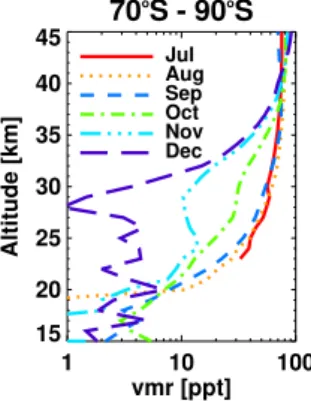
Fig. 12. Temporal evolution of mean Antarctic SO2vmr profiles in winter and spring.

ues of about 80–100 pptv (Figs. 8 and 7) at 45 km. At these altitudes, the SO₂concentrations do not show any large vari-ability with latitude. This increase of SO₂from the middle to the upper stratosphere is caused by photolysis of H₂SO₄that is released due to the evaporation of aerosols (Vaida et al., 2003; Mills et al., 2005). At altitudes of 45 km Brühl et al. (2012, Fig. 6) show values of around 50 pptv of SO_x(mostly SO2), which are considerably smaller than our data. This

can be explained by neglecting in the model SO2

photoly-sis bands in the visible and near IR (Brühl et al., 2013). The models in SPARC (2006, Fig. 6.11) show large differences at these altitudes: in the tropics three of the models underesti-mate the observed SO2 values above the mid-stratospheric

maximum, while the LASP model compares rather well. However, at 45◦_{N this model overestimates the high-altitude}

MIPAS observations by a factor of 2, while other models are still lower than the observations.

In wintertime at high latitudes the MIPAS data show the descent of enhanced upper stratospheric SO₂concentrations down to 20–25 km altitude (see Fig. 7 and blue curves in Fig. 8). On average, vmr values of 50–60 pptv are reached at 30 km, and 20–40 pptv at 25 km. This periodic effect is clearly visible in the top rows of Figs. 4 and 5. The mean evolution over the Antarctic from July to December is shown in detail in Fig. 12, which can be compared with the simu-lations shown in Mills et al. (2005, Fig. 5). In those model runs highest SO2 values of about 100 pptv at 30 km and

60 pptv at 25 km altitude are reached in the Antarctic po-lar vortex by the end of August. In the observations, high-est SO2concentrations at these altitudes are observed in July

(13)

Table 2.Major volcanic eruptions in the time period of the MIPAS measurements. General data of volcanoes are from http://www.volcano.si. edu. Injection heights and SO₂masses are based on Neely et al. (2013, Table S1) and references therein. References for additional eruptions: Soufrière Hills on 12 July 2003, Carn and Prata (2010); Soufrière Hills on 11 February 2010, Cole et al. (2010); Nabro mass, Clarisse et al. (2012); Nabro injection height, Bourassa et al. (2012) and connected discussion (Fromm et al., 2013; Vernier et al., 2013; Bourassa et al., 2013); Merapi, Surono et al. (2012). In the case of Pacaya, the SO₂mass is taken from Aura/OMI measurements on 30 May 2010 (http://so2.gsfc.nasa.gov).

Name Location Eruption date SO₂mass Injection height

[Tg] [km]

Ruang 2.3◦_{N, 125.4}◦_E _{25 Sep 2002} _0.055 ₂₀

El Reventador 0.1◦_{S, 77.7}◦_W _{3 Nov 2002} _0.096 ₁₇

Soufrière Hills 16.7◦_{N, 62.2}◦_W _{12 Jul 2003} _0.12 ₁₅

Anatahan 16.4◦_{N, 145.7}◦_E _{12 Apr 2004} _0.065 ₁₅

Manam 4.1◦_{S, 145}◦_E _{27 Jan 2005} _0.18 ₁₉

Sierra Negra 0.8◦_{S, 91.2}◦_W _{22 Oct 2005} _0.36 ₁₅

Soufrière Hills 16.7◦_{N, 62.2}◦_W _{20 May 2006} _0.2 ₂₀

Rabaul (Tavurvur) 4.3◦_{S, 152.2}◦_E _{7 Oct 2006} _0.125 ₁₇

Tair, Jebel al 15.5◦_{N, 41.8}◦_E _{30 Sep 2007} _0.08 ₁₆

Chaiten 42.8◦_{S, 72.6}◦_W _{2 May 2008} _0.01 ₁₉

Okmok 53.4◦_{N, 168.1}◦_W _{12 Jul 2008} _0.122 ₁₆

Kasatochi 52.2◦_{N, 175.5}◦_W _{7 Aug 2008} _1.7 _14–18

Sarychev 48.1◦_{N, 153.2}◦_E _{12 Jun 2009} _1.4 ₁₇

Soufrière Hills 16.7◦_{N, 62.2}◦_W _{11 Feb 2010} _0.05 ₁₅

Pacaya 14.4◦_{N, 90.6}◦_W _{28 May 2010} _0.02

Merapi 7.5◦_{S, 110.4}◦_E _{26 Oct 2010} _0.44 ₁₇

Nabro 13.4◦_{N, 41.7}◦_E _{12 Jun 2011} _1.5 _14–18

6.3 Lower stratospheric variability

In Fig. 6 we indicated the time and geographical latitude of major volcanic eruptions by orange triangles together with the initials of each volcano as specified in Table 2. As a ba-sis for this list we have taken the one compiled by Neely et al. (2013) and added further eruptions visible in the MIPAS dataset. For that purpose, the retrieval of SO₂from single MI-PAS observations (which is the topic of a separate study to be published) has been used to unambiguously assign elevated amounts of SO2to volcanic events. The clear correlation of

volcanic eruptions with elevated values of SO2in the top four

rows of Fig. 6 shows that the major variability of SO2in the

altitude range below about 22 km is determined by volcanic activity.

In the first half of the MIPAS measurement period, un-til the end of 2006, equatorial volcanic eruptions dominate the SO₂mean distribution in the lower stratosphere near the Equator (cf. Figs. 4 and 5), while during the second part mid-and high northern latitudes are mostly affected. Figure 13 compares the temporal evolution of the global SO₂content derived from MIPAS for the altitude regions 15–23 km and 20–23 km with the total injected mass as derived from nadir-sounding instruments (cf. Table 2). In the case of the larger eruptions of Kasatochi, Sarychev and Nabro, the mean SO2

content at 15–23 km in the month directly after the erup-tion is about 1–2 % of the total injected mass. As shown in Sect. 5.2, due to the similar distribution of SO2volume

mix-ing ratios between ACE-FTS and MIPAS after the eruption of Sarychev (Doeringer et al., 2012), the total mass derived from both instruments would also be comparable.

For tropical eruptions, like those of Soufrière Hills, El Reventador or Raboul, the SO₂ mass in the lower strato-sphere is of the order of 5 % or more of the total mass, likely due to the general upward transport in the tropical UTLS region. As already indicated in the plots of volume mixing ratio, the lower panel of Fig. 13 shows that altitudes above 20 km are mainly affected by the tropical eruptions before the end of 2006. Roughly about 2 % of the listed total SO₂ mass of tropical volcanoes seems to reach these high alti-tudes, while this is only about 0.1 % in the case of large mid-latitude eruptions. It should be kept in mind (1) that the MIPAS values of SO2mass in 2005 and 2006 are

underes-timated due to the sparser coverage compared to earlier and later dates, as indicated by the red crosses in Fig. 13, and (2) that due to the cloud threshold described in Sect. 3, strongly aerosol contaminated limb views are excluded from the re-trieval leading to a general underestimation of SO₂. The lat-ter effect, however, only affects few limb scans directly aflat-ter the eruption in the vicinity of the major plume such that the monthly mean values are unlikely to be disturbed.

The SO₂distributions within the tropical regions in Figs. 4 and 5 can be inspected for indications of upward transport of SO₂from the periods of volcanically enhanced values in the lower stratosphere up to the SO2maximum at around 28 km.

(14)

01-Jan

2003 01-Jan2004 01-Jan2005 01-Jan2006 01-Jan2007 01-Jan2008 01-Jan2009 01-Jan2010 01-Jan2011 01-Jan2012 0

10 20 30 40 50

Mass SO2 [Gg]

Ru Re So An Ma Si

So Ra _{Ta ChOk} Ka

Sa

So Pa Me

Na MIPAS 15-23 km Inj. mass /50 Coverage

0 20 40 60 80 100

Coverage [%]

01-Jan

2003 01-Jan2004 01-Jan2005 01-Jan2006 01-Jan2007 01-Jan2008 01-Jan2009 01-Jan2010 01-Jan2011 01-Jan2012 0

2 4 6 8 10 12

Mass SO2 [Gg]

Ru Re So An Ma Si

So_Ra Ta ChOk

Ka Sa

So Pa Me

Na MIPAS 20-23 km Inj. mass /200 Coverage

0 20 40 60 80 100

Coverage [%]

Fig. 13. Black diamonds: global monthly mean SO₂mass between 15 and 23 km (top) and 20–23 km (bottom) from MIPAS. Black bars: SO₂injection mass from Table 2 (scaling factor as given in the legend). Red: relative coverage of the latitude–height slice with MIPAS observations.

(end of 2002, beginning of 2005 and mid-2006) an upwelling of SO2-enhanced air is tentatively visible. However, due to

the processing of SO2 during the months directly after the

eruptions, much smaller values of SO2 remain for an

up-ward transport. It is probable that sulfur is transported in the form of aerosols, as has been shown, for example, in Vernier et al. (2011, Fig. 2). The time series of SO2 show that

en-hanced values at its mid-stratospheric maximum near 28 km and above are present some months after the eruptions. How-ever, as described in the following chapter there is a strong correlation with the quasi-biennial oscillation (QBO) espe-cially at those altitudes. The resulting maxima of SO₂are su-perposed to possible enhancements due to the volcanic erup-tions, and thus both effects are difficult to disentangle.

6.4 Regression analysis

In this section, the temporal development of the SO₂dataset is analysed under the consideration of a constant term a; a linear term b; several periodics; and external parameters with coefficientsc,dandeusing a multivariate fit approach as proposed by von Clarmann et al. (2010) and extended by Stiller et al. (2012). A regression function vmr(t )is fitted to the time series of SO2values at each 2 km altitude and 10◦

latitude bin:

vmr(t ) =a+bt+c1qbo1(t )+d1qbo2(t )

+c2sin2π t

T₁ +d2cos

2π t

T₁

+c3sin2π t

T0.5

+d3cos2π t

T0.5

+eF₁₀.7(t ).

(5)

Here qbo₁(t ) and qbo₂(t ) are the Singapore time series of winds at 10 hPa and 50 hPa as provided by the Free University of Berlin (http://www.geo.fu-berlin.de/en/met/ag/ strat/produkte/qbo/index.html). They are used to describe the QBO signal in the time series (Kyrölä et al., 2010). The sine and cosine terms describe annual (T₁=1 yr) and semi-annual (T0.5=0.5 yr) variability including a phase shift.

The solar radio flux at 10.7 cm (F10.7(t )) provided by the

NOAA Space Weather Prediction Center (http://www.swpc. noaa.gov) serves as proxy for solar activity (Kyrölä et al., 2010). A possible offset between P1 and P2 data is accounted for by adding a fully correlated block matrix to the P1 part of the data error covariance matrix.

In Fig. 14, results of the regression analysis are shown for exemplary latitude–height bins illustrating the influence of various partial signals. In the following, Fig. 14 is discussed together with Fig. 15, where the global distribution of the am-plitudes of the single regression functions is presented (see caption of Fig. 15 for a more detailed description).

The quality of the fit is illustrated by theχ2of the regres-sion (see plot “CHI2” in Fig. 15). In general the global fit quality is relatively homogeneous. The main exceptions are the regions of the polar upper stratosphere and the northern lowermost stratosphere with higher values of χ2. The lat-ter is probably explained by volcanic activity the influence of which was mainly concentrated at altitudes up to 20 km in the north (see Sect. 6.3). Further, influences by anthro-pogenic sources may also contribute to the higher values of χ2there. Enhancedχ2at high latitudes above 30–35 km alti-tude stem from strongly increased values of SO₂up to 120– 160 pptv during single winter months (see e.g. top row of Fig. 5), which cannot be represented adequately by the re-gression model.

The QBO signal can clearly be detected in the tropics at altitudes of 28–36 km introducing a variability in SO₂ of around±20 pptv (cf. top right panel in Fig. 15 and example “QBO” in Fig. 14). Here the major part of the QBO signal stems from qbo₁(t ), the Singapore winds at 10 hPa, whereas the winds at 50 hPa (qbo2(t )) are of minor importance. High values of SO2are correlated with the easterly phase of the

QBO. Such a QBO signal has also been observed in the case of time series of stratospheric aerosol extinction (Trepte and Hitchman, 1992; Vernier et al., 2011).

Large amplitudes (up to about 30 pptv) of the annual modes are present especially at altitudes of 25–35 km at po-lar latitudes (cf. Fig. 15). These are explained by the down-welling of SO₂-rich air from higher altitudes during winter. The N–S asymmetry with larger amplitudes at lower alti-tudes in the south are presumably due to the more persistent Antarctic polar vortex.

The mode of the semi-annual oscillation (SAO) with am-plitudes of up to 10 pptv of SO2 is visible above 30 km

al-titude at tropical and subtropical laal-titudes (Fig. 15). This mode can be identified in the example dataset for 20–30◦_S

(15)

lat: 0- 10 h:33-35km

03 04 05 06 07 08 09 10 11 12 Year 20 40 60 80 VMR [pptv] QBO

03 04 05 06 07 08 09 10 11 12 Year -40 -200 20 40 VMR [pptv] lat:-90--80 h:29-31km

03 04 05 06 07 08 09 10 11 12 Year 0 20 40 60 80 100 120 VMR [pptv] Annual

03 04 05 06 07 08 09 10 11 12 Year -60 -40 -200 20 40 60 VMR [pptv] lat:-30--20 h:41-43km

03 04 05 06 07 08 09 10 11 12 Year 60 80 100 120 VMR [pptv] Semi-annual

03 04 05 06 07 08 09 10 11 12 Year -40 -200 20 40 VMR [pptv]

lat:-10- 0 h:41-43km

03 04 05 06 07 08 09 10 11 12 Year 40 60 80 100 120 140 VMR [pptv] F10.7

03 04 05 06 07 08 09 10 11 12 Year -60 -40 -200 20 40 60 VMR [pptv] lat:-60--50 h:25-27km

03 04 05 06 07 08 09 10 11 12 Year 0 20 40 VMR [pptv] Linear

03 04 05 06 07 08 09 10 11 12 Year 0 20 40 VMR [pptv] lat:-60--50 h:41-43km

03 04 05 06 07 08 09 10 11 12 Year 40 60 80 100 120 VMR [pptv] Linear

03 04 05 06 07 08 09 10 11 12 Year 40 60 80 100 120 VMR [pptv]

lat: 0- 10 h:21-23km

03 04 05 06 07 08 09 10 11 12 Year 20 40 60 80 100 VMR [pptv] Linear

03 04 05 06 07 08 09 10 11 12 Year 20 40 60 80 100 VMR [pptv]

Fig. 14.Time series of multivariate fit results illustrating prominent parameters at different latitude/height regions. Marks along thex axes indicate 1 January of each year. For each parameter, two plots are grouped together: the upper one contains the measured dataset in red and the fit in black for the region as specified in the title; the lower plot illustrates the separate weight of the dedicated parameter listed in the title. Left, rows 1 and 2, linear combination of Singa-pore winds at 10 and 50 hPa; left, rows 3 and 4, annual variation; left, rows 5 and 6, semi-annual variation; left, rows 7 and 8, solar F₁₀.7flux; right column, linear trend and bias.

a second, smaller peak in the second half of each year. Such a seasonal asymmetry with stronger variation during the first cycle has been described as typical feature of the equato-rial SAO (Delisi and Dunkerton, 1988; Garcia et al., 1997). Further, a latitudinal asymmetry of the SAO with stronger intensity southwards of the Equator, as indicated in Fig. 15, has been observed previously in observations of temperature and wind (Belmont and Dartt, 1973; Ray et al., 1998). The global distribution of the reconstructed linear slope is pre-sented in Fig. 15 (bottom right). It shows generally a slight positive trend at all altitudes in the northern and, with larger values, below about 32 km in the southern extra-tropical

lat--50 0 50

Latitude [deg] 15 20 25 30 35 40 45 Altitude [km] CHI2 0 20 40 60 80 100 120 140

-50 0 50

Latitude [deg] 15 20 25 30 35 40 45 Altitude [km] QBO [pptv] 0 5 10 15 20 25

-50 0 50

Latitude [deg] 15 20 25 30 35 40 45 Altitude [km] ANNUAL [pptv] 0 5 10 15 20 25 30

-50 0 50

Latitude [deg] 15 20 25 30 35 40 45 Altitude [km] SEMI-ANNUAL [pptv] 0 5 10 15

-50 0 50

Latitude [deg] 15 20 25 30 35 40 45 Altitude [km] F10.7 [pptv] -20 -10 0 10 20

-50 0 50

Latitude [deg] 15 20 25 30 35 40 45 Altitude [km]

LINEAR SLOPE [pptv/dec]

-40 -20 0 20 40

Fig. 15. Global overview of the fit RMS (top left), the amplitudes of various fit parameters and the linear trends (bottom right). For “QBO” and “F₁₀.7”, the amplitude is defined as the semi-difference between maximum and minimum of the fitted time series of Singa-pore winds and solarF₁₀.7flux, respectively. For “F₁₀.7” the sign indicates a positive or negative correlation with the solar cycle.

-50 0 50

|LINEAR SLOPE|/σ

0 1 2 3 4 5

-50 0 50

Latitude [deg] 15 20 25 30 35 40 45 Altitude [km] |F10.7|/σ 1 2 3 4 5

-50 0 50

LINEAR SLOPE > 2σ [pptv/dec]

-40 -20 0 20 40

-50 0 50

F10.7 > 2σ [pptv]

-20 -10 0 10 20

Fig. 16. Top: significance in multiples of the estimated error of the model error corrected linear slope (left) and theF₁₀.7 amplitude (see caption of Fig. 15 for definition) (right). Bottom: remaining values with a significance>2σ.

itudes. Negative trends are mainly visible at higher altitudes in the southern subtropics and mid-latitudes and at lower al-titudes in the tropics. Single examples for time series indicat-ing stronger positive and negative trends at different altitudes in the southern mid-latitudes are shown in Fig. 14. Here at 25–27 km altitude, a positive trend is visible for the whole dataset, and even when considering only data after, for ex-ample, 2007. At 41–43 km the data show a general decrease until about 2009 and a levelling-off afterwards. As discussed above, this correlates also with theF10.7flux time series, and