www.hydrol-earth-syst-sci.net/16/1259/2012/ doi:10.5194/hess-16-1259-2012
© Author(s) 2012. CC Attribution 3.0 License.
Earth System
Sciences
Baseflow simulation using SWAT model in an inland river basin in
Tianshan Mountains, Northwest China
Y. Luo1, J. Arnold2, P. Allen3, and X. Chen1
1State Lab of Desert and Oasis Ecology, Xinjiang Institute of Ecology and Geography, Chinese Academy of Sciences, 830011
Urumqi, China
2Grassland Soil and Water Research Laboratory, USDA-ARS, Temple, TX 76502, USA 3Department of Geology, Baylor University, Waco, TX 76798, USA
Correspondence to:Y. Luo ([email protected])
Received: 28 October 2011 – Published in Hydrol. Earth Syst. Sci. Discuss.: 26 November 2011 Revised: 19 March 2012 – Accepted: 31 March 2012 – Published: 27 April 2012
Abstract.Baseflow is an important component in hydrolog-ical modeling. The complex streamflow recession process complicates the baseflow simulation. In order to simulate the snow and/or glacier melt dominated streamflow reced-ing quickly durreced-ing the high-flow period but very slowly dur-ing the low-flow period in rivers in arid and cold northwest China, the current one-reservoir baseflow approach in SWAT (Soil Water Assessment Tool) model was extended by adding a slow- reacting reservoir and applying it to the Manas River basin in the Tianshan Mountains. Meanwhile, a digital filter program was employed to separate baseflow from stream-flow records for comparisons. Results indicated that the two-reservoir method yielded much better results than the one-reservoir one in reproducing streamflow processes, and the low-flow estimation was improved markedly. Nash-Sutcliff efficiency values at the calibration and validation stages are 0.68 and 0.62 for the one-reservoir case, and 0.76 and 0.69 for the two-reservoir case. The filter-based method estimated the baseflow index as 0.60, while the model-based as 0.45. The filter-based baseflow responded almost immediately to surface runoff occurrence at onset of rising limb, while the model-based responded with a delay. In consideration of wa-tershed surface storage retention and soil freezing/thawing effects on infiltration and recharge during initial snowmelt season, a delay response is considered to be more reasonable. However, a more detailed description of freezing/thawing processes should be included in soil modules so as to deter-mine recharge to aquifer during these processes, and thus an accurate onset point of rising limb of the simulated baseflow.
1 Introduction
Baseflow is a streamflow component which reacts slowly to rainfall and is usually associated with water discharged from groundwater storage (Eckhardt, 2008). Knowledge about baseflow is useful in assessing water quality, fore-casting streamflow, allocating water supply, and designing hydropower plants (Tallaksen, 1995) under low-flow con-ditions. When, where, and how much streamflow can be attributed to groundwater discharge is thus practically important.
The Soil and Water Assessment Tool (SWAT, Arnold and Fohrer, 2005) uses a conceptual linear one-reservoir (shal-low aquifer storage) approach to simulate basef(shal-low. SWAT partitions groundwater into two aquifer systems: a shallow aquifer which contributes baseflow to streams within the wa-tershed, and a deep aquifer which contributes baseflow to streams outside the watershed and can be considered lost from the system (Arnold et al., 1993). While the shallow aquifer-baseflow was properly reproduced by SWAT (Arnold et al., 2000; Jha et al., 2007), weaker simulation of baseflow was found as well (Kalin and Hantush, 2006; Srivastva et al., 2006). Peterson and Hamlett (1998) found that SWAT was not able to simulate baseflow due to the presence of soil fragipans. Chu and Shirmohammadi (2004) found that the baseflow was not simulated properly for an extremely wet year. Wu and Johnston (2007) found underestimated baseflow by SWAT especially during dry years in a Great Lake watershed and indicated that this is primarily due to the long temporal lag between winter snowpack accumulation and spring snow melting events. Luo et al. (this study) found underestimation of baseflow during the low-flow period in the Manas River Basin in northern Tianshan Mountains using SWAT2005. For the glaciated Oigaing River basin in west-ern Tianshan and the Ala Archa River basin also in north-ern Tianshan, Aizen et al. (2000) used one linear reservoir to generate baseflow and found that the discharge was underes-timated during autumn-winter as well. The steep slopes of the river basins in Tianshan Mountains, the quick recession of surface runoff, and the sluggish and stable baseflow pro-cesses might indicate a quick percolation of rainfall and snow and glacier melt waters during the summertime to an under-ground storage which releases slowly during the wintertime. Nathan and McMhon (1990) indicated that baseflow itself may be composed of a number of components, each of which may vary seasonally with different recession constants. Sup-posedly, an additional slow release pool may improve the low-flow estimation for rivers in the Tianshan Mountains, which is not present in both Aizen’s (2000) model and the SWAT model.
Therefore, the main objective of this paper is to develop a two-reservoir approach for baseflow simulation in SWAT and use the model to simulate the streamflow process that is characterized by combined steep and sluggish recession stages of the receding limb in an arid and cold inland river basin in the Tianshan Mountains, northwest China.
2 Materials and methods
2.1 Baseflow modeling in SWAT
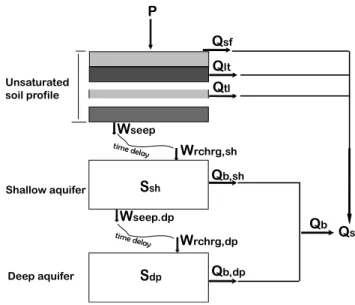
In the SWAT model, water routed through channel system to the gauges consists of four components: direct surface runoff (Qsf), lateral flow from unsaturated soil profiles (Qlt),
drainage from tiles (Qtl), and baseflow from underground
Ssh
Sdp
Qsf
Qlt
Wrchrg,sh
Qb,sh
Wrchrg,dp
Qb,dp
Qb
P
Qs
Shallow aquifer
Deep aquifer Unsaturated
soil profile Qtl
Wseep
Wseep.dp time delay
time delay
Fig. 1 Schematic of streamflow components in SWAT model
Fig. 1. Schematic of streamflow components in the SWAT model. Note:P is precipitation;Qltis lateral soil water flow;SshandSdp are water storages of the shallow and deep aquifer, respectively; other symbols are mentioned within the text.
storage (Qb) (Fig. 1). Modeling of the direct surface runoff,
the lateral soil flow, and the tile drainage are described in de-tail in theoretical documents of SWAT model (Neitsch et al., 2005) and thus will not be described repeatedly here. The baseflow simulation will be focused hereafter.
SWAT differentiates the underground storage into two por-tions, shallow aquifer and deep aquifer. The shallow aquifer receives recharge from the unsaturated soil profile percola-tion. An exponential decay weighting function is utilized to account for the time delay in aquifer recharge once the wa-ter exits the soil profile (Neitsch et al., 2005). The delay function accommodates situations where the recharge from the soil zone to the aquifer is not instantaneous, i.e. 1 day or less. The recharge to aquifer on a given day is calculated as below:
Wrchrg,i =
1 − exp
− 1
δgw,sh
Wseep
+exp
− 1
δgw,sh
Wrchrg,i−1 (1)
whereWrchrgis the amount of recharge entering the aquifers
(mm H2O day−1),δgw,shis the delay time of the overlying
ge-ologic formations (days),Wseepis the total amount of water
exiting the bottom of the soil profile (mm H2O day−1);
sub-scriptions “seep” indicates seepage water exiting bottom of unsaturated soil profile, “rchrg” indicates recharge,i is the sequential number of days, and “sh” indicates the shallow aquifer storage.
aquifer due to percolation to the deep aquifer on a given day is given by:
Wseep,dp,i = βdpWrchrg,i (2)
whereβdp is a coefficient of shallow aquifer percolation to
deep aquifer, and subscription “dp” indicates deep aquifer. The amount of recharge entering the shallow aquifer is:
Wrchrg,sh,i = Wrchrg,i − Wseep,dp,i. (3)
Baseflow generated from the shallow aquifer on a given dayi
under influence of recharge is given as below (Neitsch et al., 2005):
Qb,sh,i = Qb,sh,i−1 · exp −αgw,sh · 1t +Wrchrg,sh,i·
1 − exp −αgw,sh · 1t
(4) whereQb,sh,i is the baseflow from the shallow aquifer on
dayi(mm H2O day−1), and “b” indicates baseflow, and1t
is the step time length. Daily time step is used in this study. When only one reservoir is used, the baseflow is equal to that from the shallow aquifer.
Qb,i = Qb,sh,i (5)
SWAT assumes that water entering the deep aquifer is not considered in the future water budget calculations and can be considered lost from the system (Neitsch et al., 2005). This study uses the deep aquifer as a parallel reservoir generating the baseflow, which enters the channel system eventually, to improve the streamflow process simulation in the low-flow period. When the two-reservoir approach is used, baseflow from the shallow aquifer is expressed as in Eq. (4), and fol-lowing Eqs. (1) and (2), the recharge to and baseflow from the deep aquifer are given by Eqs. (6) and (7), respectively.
Wrchrg,dp,i = Wrchrg,dp,i−1 · exp
− 1
δgw,dp
+Wseep,dp,i ·
1 − exp
− 1
δgw,dp
(6)
Qb,dp,i = Qb,dp,i−1 · exp −αgw,dp · 1t
+Wrchrg,dp,i · 1 − exp −αgw,dp · 1t (7)
whereWrchrg,dpis the amount of recharge entering the deep
aquifer (mm H2O day−1),δgw,dpis the delay time or drainage
time of the deep aquifer geologic formations (days),Wseep,dp
is the total amount of water exiting the bottom of the shallow aquifer (mm H2O day−1),Qb,dpis baseflow component from
deep aquifer. The total baseflow is then given as below:
Qb,i = Qb,sh,i + Qb,dp,i. (8)
When the shallow storage reservoir is used only to generate baseflow, recharge to the deep aquifer is disabled. When both aquifers are used to generate baseflow, the parameterβdpis
determined through calibration. Other parameters to be cal-ibrated for baseflow modeling include the delay timeδgw,sh,
δgw,dp, the recession constantsαgw,shandαgw,dp.
2.2 Baseflow separation using automated digital filter
In consideration of difficulties in the measurement of base-flow, a third-party approach, the digital filter-based pro-gram, is used to separate baseflow from streamflow records for comparison purposes. This baseflow separation proce-dure is based on a recursive digital filter commonly used in signal analysis and processing (Lyne and Hollick, 1979). It was used by Nathan and McMahon (1990), Arnold and Allen (1999) and Szilagyi et al. (2003, 2004), among others. This technique is, in fact, arbitrary and physically unrealistic. However, it does provide a subjective and repeatable estimate of baseflow that is easily automated (Nathan and McMahon, 1990). The filter given by Lyne and Hollick (1979) is ex-pressed as below:
Qsf,i = λQsf,i−1 +
1 + λ
2 Qs,i − Qs,i−1
(9) where Qsf and i are defined as before, Qs is the surface
runoff, andλis the filter parameter. Baseflow is calculated as below:
Qb,i = Qs,i − Qsf,i (10)
whereQbis defined as before.
An automatic baseflow filter program (Arnold et al., 1995, http://swatmodel.tamu.edu/software/ baseflow-filter-program,2011) is used to separate base-flow from the daily streambase-flow records from 1961 to 1999 in Manas River Basin (MRB).
2.3 Watershed and data description
Model setup
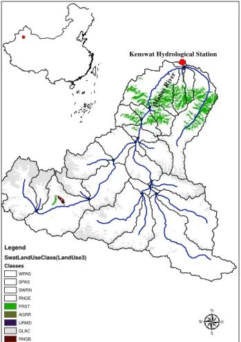
MRB is located at the northern side of the middle Tianshan Mountains, northwest China (Fig. 2). MRB originates from the Yilianhabierga Mountain, runs 160 km to the outlet at Kenswat Hydrological Station (KHS, 85◦
57′
E, 43◦
58′
), and runs further 240 km through the oasis and the desert and fi-nally merges into Manas Lake. The catchment area of the MRB above the outlet KHS is 5163 km2.
Maps of a 1:250 000 DEM, a 1:100 000 land cover, and the China Glacier Inventory (CGI) were used to setup the Arc-SWAT2005. The CGI data used as the initial glacier layout were mainly derived from topographical maps (1:100 000) based on aerial photos acquired during 1962–1977 (Shang-guan et al., 2009). Eventually, the watershed is delineated into 27 subbasins and 163 Hydrological Response Units (HRUs). Each subbasin is divided into ten bands with equal elevation increment for simulating the snow and glaciers.
(1) Topography and land cover
&
-Kenswat Guage Kenswat Hydrological Station
Man as R
iver
Legend
SwatLandUseClass(LandUse3)
Classes WPAS SPAS SWRN RNGE FRST AGRR URMD GLAC
RNGB
µ
%
,
Ken s wat Gu a g e
Manas River
Text
Fig. 2. The Manas River basin and subbasin delineation map (the upper-left small figure is the sketch map of China indicating the location of the study area).
within a subbasin are significant. On average, the difference is 2561 m, with the biggest at 3876 m for the subbasin 11 and the smallest at 448 m for the subbasin 1. The land cover types include range grassland of 8.11 % elevation band 2500–3500 m a.s.l., short bushes of 39.1 % within the eleva-tion band of 1500–2500 m a.s.l., and forest of 5.32 % within the below the elevation of 1500 m a.s.l., bare land of 33.58 %, and glaciers. Among the 163 HRUs, there are 28 glacierized ones with total glacier area of 717 km2. Ratios of glacier area to subbasin area range from 0.7 % for the subbasin 4 to 51.2 % for the subbasin 22, with a mean ratio of 13.9 % over the basin. Watershed glacier processes simulation was detailed in Luo et al. (this study).
(2) Soils
The main soils in the basin include alpine meadow soil, subalpine meadow soil, subalpine meadow and steppe soil, mountain chernozem soil, mountain grey cinnamon soil, mountain chestnut soil, which take account of 36 %, 11 %,
42 %, 1 %, 7 %, and 3 % of the basin area, respectively. Tex-tures and properties of these soils were derived from the field-collected and lab- tested data of the publication “Soils in Xinjiang (technical report)”.
(3) Climate
The Shihezi Weather Station (SWS, 43◦
29′
N, 87◦
06′
E) is located below the outlet with an elevation of 444 m a.s.l. The daily meteorological data include maximum and minimum temperatures, wind speed at 10 m height, relative humidity, precipitation, and 20 cm-pan evaporation from 1961 to 1999. This area displays an alpine climate, very cold winter and moderate summer temperatures. The mean high temperature is 39.6◦
C, the low−31.7◦C, and the daily average 7.0◦C.
The mean annual precipitation is 196 mm and the pan evap-oration 1714 mm.
For each subbasin, a virtual weather station (VWS) is de-fined. For each VWS, the temperature and precipitation data were derived from the SWS by using the temperature and precipitation lapse rates. Default value −6◦C km−1 in the
SWAT model was used for the temperature lapse rate,and 45 mmkm−1was used for the precipitation lapse rate (Luo et al.,
this study).
(4) Streamflow
Daily streamflow records at the KHS from 1961–1999 were used. The mean daily discharge rate is 39.3 m3s−1and the
average annual volume 12.15×10⁸m3. The recorded maxi-mum annual volume is 20.08×10⁸m3in 1999 and the min-imum 9.39×10⁸m3in 1983. The flow volume from June to
August takes account of 70.5 % of the annual value and of 28.9 % and 25.9 % for July and August, respectively. Dur-ing the seven months from October to the next April, flow volume accounts for 15.9 % of the year with the monthly ra-tio decreasing from 4.2 % in September to 1.2 % in February and then going up gradually to 2.0 % in April.
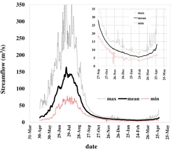
MRB is snow and glacier melt dominated. Snowmelt starts usually in late April or early May, glacier melts as snowpack depletes, and streamflow starts to rise consistently till peak discharge in late July. Glacier melt contribution ceases in late September. As temperature falls below 0◦C, a new snow
season begins, and the direct surface runoff to streamflow ceases. Steep rising and receding streamflow curve is then followed with an almost flat low-flow line during the winter and spring seasons, while the streamflow is very stable and has quite a long duration (Fig. 3), which is a common feature for rivers in northwest China.
0 50 100 150 200 250 300 350 31 -Mar 30 -Ap r 30 -M ay 29-J un 29 -Ju l 28-Aug 27 -S ep 27 -O ct 26 -No v 26 -De c 25 -Jan 24 -Fe b 26 -Mar 25 -Ap r 25 -M ay Str e amflow (m 3/s ) date
max mean min
0 5 10 15 20 25 30 35 27-S ep 27-Oc t 26-N ov 26-De c 25-Jan 24-F eb 26-M ar 25-A p r 25-M ay max mean min
Fig. 3.The measured mean streamflow process of the Manas River, Tianshan, Northwest China (max = the maximum daily flow rate; min = the minimum daily flow rate; mean = the mean daily flow rate from 1961 to 1999).
both the Nash-Sutcliffe efficiency (NSE) and Percent Bias (PBIAS) indices (Moriasi et al., 2007).
NSE = 1 −
n P
1
Qobsi − Qsimi 2
n P
i
Qsimi − Qmean2
(11)
PBIAS =
n P
1
Qobsi − Qsimi
n P
i
Qobsi
×100 (12)
whereQobsi is thei-th observation for the daily flow,Qsimi is thei-th simulation value for the daily flow,meanis the mean of observed data for the daily flow, andnis the total number of the daily flow observations.
NSE indicates how well the plot of observed versus simu-lated data fits the 1:1 line. NSE ranges between−∞and 1.0
(1 inclusive), with NSE = 1 being the optimal value. PBIAS measures the average tendency of the simulated data to be larger or smaller than their observed counterparts. The opti-mal value of PBIAS is 0.0, with low-magnitude values indi-cating accurate model simulation (Morasi et al., 2007).
3 Results
Parameters calibrated for baseflow components are listed in Table 1 for reference. In case one-reservoir was used only, it was assumed that water exiting the bottom of the unsaturated
Table 1.Baseflow parameter values for one reservoir and two reser-voir approaches in SWAT and the automated baseflow filter program for the Manas River basin, Tianshan, China.
Model Parameter unit Initial Calibrated
value value
One δgw,sh day 10–30 15
reservoir αgw,sh – 0–1 0.4
β – 0 0
Two δgw,sh day 10–30 15
reservoirs αgw,sh – 0–1 0.4
δgw.dep day 10–300 127
αgw,dp – 0–1 0.05
β – 0–1 0.4
Filter λ – 0.925
program α – 0.018
baseflow days day 127.9
soil profiles recharged the shallow aquifer only. When the two-reservoir method was employed, it was found that 40 % of recharge to the deep aquifer was proper to match the mea-sured streamflow during low-flow period. The deep aquifer has a much longer delay time for recharge and a much slower recession rate than the shallow aquifer. Parameters for the baseflow filter are also listed in Table 1. It is interesting to notice that using the baseflow days given by the filter pro-gram (Arnold et al., 1995; Arnold and Allen, 1999) as the recharge delay time of the deep aquifer in the two-reservoir approach simulated the stream flow during low-flow period very well.
Figure 4 demonstrates the comparison of stream flows among those measured and simulated. A five-year clip was taken from the whole simulation period of 39 yr to give a clearer picture. The two-reservoir method improved the low-flow simulation remarkably in vision. Statistical indices NSE and PBIAS indicate that the two-reservoir method yielded “good” or even “very good” results in the sense of either NSE or PBIAS following the rating rules given by Moriasi et al. (2007), which are better than the one-reservoir method, Table 2.
Fig. 4. Comparison of simulated to measured streamflow processes at validation stage, the simulation started in 1961 (ROF = runoff; m = measured; 1R, = one-reservoir method; 2R = two-reservoir method).
Table 2.The NSE and PBIAS for the simulated discharge by SWAT using the one-reservoir and two-reservoir baseflow approaches in the Manas River basin, Tianshan, China.
NSE Rating∗ PBIAS(%) Rating∗
One-reservoir
calibration 0.68 Good −4.0 Very
validation 0.62 Satisfactory −3.5 good
overall 0.65 Good −3.7
Two-reservoir
calibration 0.76 Very good −2.6 Very
validation 0.69 Good −3.6 good
overall 0.72 Good −3.2
∗The rating is based on rules given by Moriasi et al. (2007). 4 Discussion
The annually averaged baseflow volumes given by different approaches were listed in Table 4. The one-reservoir and two-reservoir approaches produced similar results in annual baseflow volumes. The digital filter program gave a much larger baseflow volume than the model-based methods. The model-based baseflow volume accounted for 45 % of the an-nual flow volume, while the filter-based 60 %. Among the model-based baseflow, shallow aquifer contributed 58 %, and the deep aquifer 42 %. According to the recharge partition coefficient, these should be 60 % and 40 %, respectively. The minor difference was attributed to a portion of the shallow aquifer storage depleted during the simulation period. For the deep aquifer, its storage fluctuated seasonally while equi-librium was maintained, as the simulation revealed.
The observed streamflow flattened out with delayed flow supply from deeper subsurface stores and eventually became nearly constant, which is sustained by outflow from ground-water storage (Fig. 3). Figure 4 illustrates the baseflow
Table 3.Statistical analysis for the baseflow components and index for Manas River basin, Tianshan, northwest China.
max min mean stdev
Flow volumes (109m3)
Runoff (M) 2.020 0.936 1.214 0.220
Runoff (S)-1R 1.764 0.900 1.251 0.183 Runoff (S)-2R 1.755 0.926 1.252 0.174
processes. When only one-reservoir was used, the base flow was underestimated as shown in Fig. 4. The ob-served mean daily flow rate was 9.8 m3s−1and the volume
of 1.88×10⁸m3 during the period from October to April,
while the simulated value was 3.0 m3s−1 and the volume
of 0.58×10⁸m3for the same period. Similar results were
also found for Oigaing River basin in western Tianshan and the Ala Archa River basin in northern Tianshan when a one-reservoir baseflow approach was used (Aizen et al., 2000). The steep slopes of the MRB (Luo et al., this study), the quick recession of surface runoff, and the sluggish and sta-ble baseflow processes during late autumn and late spring (Fig. 1) indicate a quick percolation of rainfall and snow and glacier melt waters during the summertime to an under-ground storage which releases slowly during the wintertime, as found by isotopic measurements in the Wind River Range of Wyoming of US (Cable et al., 2011). When the deep aquifer was employed as an additional slow release pool, the baseflow simulation was improved remarkably, as demon-strated in Figs. 5 and 6a and b.
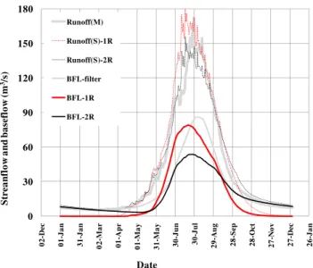
The model- and filter-based daily baseflow processes were averaged over the period from 1966 to 1999 (Fig. 6). The simulated streamflow peak time seemed to shift a little ear-lier. Nevertheless, the simulated rising receding limbs match the measured ones well.
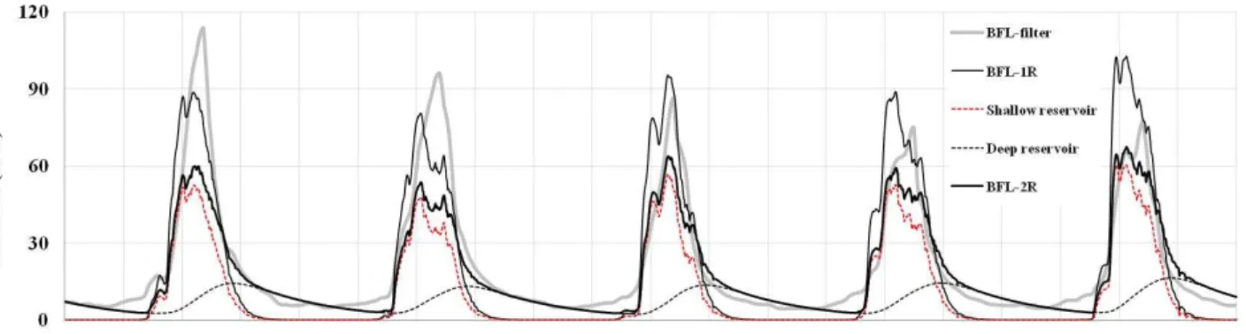
Fig. 5. Clip illustration of the seasonal baseflow processes generated by model- and filter-based approaches, the whole period covered 1961–1999, 1961 as the year 1 (BFL = baseflow; filter = filter-based baseflow separation program; 1R = one-reservoir approach; 2R = two-reservoir approach; Shallow two-reservoir = the shallow aquifer two-reservoir generated baseflow; Deep two-reservoir = the deep aquifer two-reservoir gener-ated baseflow).
0 4 8 12 16
0 4 8 12 16
M
o
nthl
y
m
e
a
n
runo
ff-m
ea
su
red
(m
3
/s
)
Monthly mean runoff-1R (m3/s) runoff 1:1
(a)
0
4 8 12 16
0 4 8 12 16
M
o
nthl
y
m
e
a
n
runo
ff-m
ea
su
red
(m
3
/s
)
Monthly mean runoff-2R (m3/s) runoff 1:1
(b)
Fig. 6. Comparison of the simulated and measured monthly averaged low-flow discharge rates. (a)The one-reservoir approach was used;
(b)the two-reservoir approach was used.
underestimation of streamflow, while the two-reservoir method reproduced the streamflow properly. Combination of the quick release reservoir and the slow release reservoir matched both the quick ad sluggish receding stages of re-cession limb of the streamflow very well. During the quick receding stage, the quick-release pool played a more impor-tant part than the slow-release pool and vice-versa during the sluggish stage (Figs. 3 and 7).
The filter-based baseflow started to rise earlier, reached its peak later, and turned to low-flow stage earlier again than the based (Fig. 6). The earlier peak time of the model-based baseflow might be attributed to streamflow peak time shift.
Onset points of rising limbs are worth noting (Figs. 4 and 6). The filter-based baseflow responds to runoff oc-currence immediately at the onset of rising limb. The
model-based baseflow responds with a delay. The Manas River basin is snow and glacier melt dominated. Snowmelt starts usually in the middle of April. Infiltration in frozen soils is affected by soil permeability, water content, re-peated thawing and refreezing, and many other factors and their complex interactions (French and Binley, 2004; Stahli, 2005). Experimental (Hayashi et al., 2003; Iwata et al., 2010) and mathematical (Flerchinger and Saxton, 1989; Zhao and Gray, 1999) investigations revealed the impeding effects of frozen soil layer to snowmelt infiltration, and hence the po-tential recharge to aquifers. As a matter of fact, baseflow should respond with a delay to the snowmelt, other than im-mediately, as given by the filter-based approach (Fig. 6). This is achieved by the SWAT model through a simple assumption of no water flow during the frozen season. An issue remain-ing to be addressed is infiltration to and recharge from the
0 30 60 90 120 150 180
02
-D
ec
01-Jan
31-Jan
02-M
ar
01-A
p
r
01-M
ay
31-M
ay
30-J
u
n
30
-Ju
l
29-A
u
g
28-S
ep
28-O
ct
27-N
ov
27
-D
ec
26-Jan
S
tr
e
an
fl
ow
an
d
b
a
se
fl
ow (
m
3/s)
Date
Runoff(M)
Runoff(S)-1R
Runoff(S)-2R
BFL-filter
BFL-1R
BFL-2R
Fig. 7.Comparison of the averaged daily baseflow processes gener-ated by different baseflow approaches (BFL = baseflow; 1R = one-reservoir approach; 2R = two-one-reservoir approach; filter = filter-based baseflow separation approach).
soil profile during freezing and thawing, and eventual deter-mination of the onset point of rising limb (Eqs. 4 and 7). This needs more detailed description of soil freezing/thawing pro-cesses, which are described insufficiently in most watershed hydrological models.
Both the model-based and the filter-based approaches cap-tured the reflection point of recession limb in late Septem-ber, when direct surface runoff usually ceases to discharge the aquifers.
Compared to the one-reservoir method, the two-reservoir method requires three extra parameters to calibrate. This case study revealed that the extra parameters will not provide too much extra work for calibration if proper steps are followed. Firstly, calibrate the parameters with recharge to deep aquifer disabled, and optimize parameters with the quick rising and receding limbs as target. Then, activate the recharge to the deep aquifer and optimize the three parameters for the slow release pool. An important reminder is that the slow-release pool has a longer recharge delay time and smaller reces-sion constant than the quick-release pool. And, as aforemen-tioned, the baseflow days given by the filter-based program can be a tip for calibrating the delay time. The recession constant given by the filter program can also be an initial es-timation of the recession constant of the slow-release pool.
5 Conclusions
In this study we presented a methodology to simulate base-flow processes by adding a slow-reacting linear reservoir to the available quick-reacting reservoir of baseflow generation in the SWAT model. The baseflow-enhanced SWAT model
Table 4.Statistical analysis for the baseflow components and base-flow index for Manas River basin, Tianshan, northwest China.
max min mean stdev
Flow volumes (109m3)
BFL-filter 1.071 0.5.82 0.720 0.111
BFL-1R 0.810 0.3.57 0.563 0.087
BFL-2R 0.802 0.3.81 0.564 0.080
BFL-sh 0.471 0.1.94 0.325 0.054
BFL-dp 0.332 0.1.87 0.239 0.030
Baseflow index
BFI-Filter 0.64 0.52 0.60 0.03
BFI-1R 0.51 0.39 0.45 0.03
BFI-2R 0.50 0.38 0.45 0.03
note: Runoff = streamflow; BFL = baseflow; sh = shallow aquifer reservoir; dp = deep aquifer reservoir; filter = filter-based baseflow separation program; 1R = one-reservoir approach; 2R = two-reservoir approach; baseflow index = proportion of baseflow components of the runoff; SRF = direct surface runoff.
was used to simulate the streamflow process in the snow and glacier melt-dominated Manas River basin in the Tianshan Mountains, where the streamflow process is featured with steeper rising and receding limbs from May to September, and a quite flatter recession from October to April. The fol-lowing conclusions were achieved.
Combination of two linear reservoirs lead to the best re-sults in reproducing the streamflow processes. The Nash-Sutcliff efficiency values at the calibration and validation stages are 0.68 and 0.62 for the one-reservoir case, and 0.76 and 0.69 for the two-reservoir case; the percent bias for both cases is better than−4 %. The two-reservoir approach im-proved the streamflow flow remarkably, especially the low-flow.
The filter-based approach responds immediately to sur-face runoff occurrence at the onset of rising limb, while the model-based approaches respond with a delay. In consider-ation of retention of surface storage and impeding effects of frozen soil layers on infiltration during the initial snowmelt stage, a delay response is believed more reasonable. Mean-while, it is suggested that freezing/thawing processes be in-cluded in soil modules to determine recharge to the aquifers and hence, the proper timing of baseflow response. The filter-and model-based methods gave similar surface runoff cessa-tion points which are in late September.
The filter-based method estimated the baseflow index as 0.60, while the model-based as 0.45 in the Manas River basin. it cannot be decided which is more representative due to the unavailability of baseflow measurements.
Acknowledgements. This paper is partially funded by the 973
Edited by: A. Gelfan
References
Aizen, V. B., Aizen, E., Glazirin, G., and Loaiciga, H. A.: Simu-lation of daily runoff in Central Asian alpine watersheds, J. Hy-drol., 238, 15–34, 2000.
Arnold, J. and Allen, P.: Automated methods for estimating base-flow and ground water recharge from streambase-flow records, J. Am. Water Resour. Assoc., 35, 411–424, 1999.
Arnold, J. and Fohrer, N.: SWAT2000: Current capabilities and research opportunities in applied watershed modeling, Hydrol. Process., 19, 563–572, 2005.
Arnold, J., Allen, P., and Bernhardt, G.: A comprehensive surface-groundwater flow model, J. Hydrol., 142, 47–69, 1993. Arnold, J., Allen, P., Muttiah, R., and Bernhardt, G.: Automated
base flow separation and recession analysis techniques, Ground Water, 33, 1010–1018, 1995.
Arnold, J., Muttiah, R., Srinivasan, R., and Allen, P.: Regional esti-mation of base flow and groundwater recharge in the upper Mis-sissippi basin, J. Hydrol., 227, 21–40, 2000.
Cable, J., Ogle, K., and Williams, D.: Contribution of glacier melt water to streamflow in the Wind River Range, Wyoming, inferred via a Bayesian mixing model applied to isotopic measurements, Hydrol. Process., 25, 2228–2236, doi:10.1002/hyp.7982, 2011. Chu, T. W. and Shirmohammadi, A.: Evaluation of the SWAT
model’s hydrology component in the Piedmont physiographic re-gion of Maryland, Trans. ASAE, 47, 1057–1073, 2004. Eckhardt, K.: A comparison of baseflow indices, which were
cal-culated with seven different baseflow separation methods, J. Hy-drol., 352, 168–173, 2008.
Fenicia, F., Savenije, H. H. G., Matgen, P., and Pfister, L.: Is the groundwater reservoir linear? Learning from data in hy-drological modelling, Hydrol. Earth Syst. Sci., 10, 139–150, doi:10.5194/hess-10-139-2006, 2006.
Ferket, B. V. A., Samain, B., and Pauwels, V. R. N.: Internal vali-dation of conceptual rainfall-runoff models using baseflow sepa-ration, J. Hydrol., 381, 158–173, 2010.
Flerchinger, G. N. and Saxton, K. E.: Simultaneous heat and wa-ter model of a freezing snow-residue-soil system I. Theory and development, Trans. Am. Soc. Agr. Eng., 32, 565–571, 1989. French, H. and Binley, A.: Snowmelt infiltration: monitoring
tem-poral and spatial variability using time-lapse electrical resistivity, J. Hydrol., 297, 174–186, 2004.
Hayashi, M., van der Kamp, G., and Schmidt, R.: Focused infiltra-tion of snowmelt water in partially frozen soil under small de-pressions, J. Hydrol, 270, 214–229, 2003.
Hilberts, A. G. J., van Loon, E. E., Troch, P. A., and Paniconi, C.: The hillslope-storage Boussinesq model for non-constant bedrock slope, J. Hydrol., 291, 160–173, 2004.
Iwata,Y., Hayashi, M., Suzuki, S., Hirota, T., and Hasegawa, S.: Effects of snow cover on soil freezing, water movement, and snowmelt infiltration: A paired plot experiment, Water Resour. Res., 46, W09504, doi:10.1029/2009WR008070, 2010. Jha, M., Gassman, P. W., and Arnold, J. G.: Water quality
model-ing for the Raccoon River watershed usmodel-ing SWAT2000, Trans. ASABE, 50, 479–493, 2007.
Kalin, L. and Hantush, M. H.: Hydrologic modeling of an eastern Pennsylvania watershed with NEXRAD and rain gauge data, J.
Hydrol. Eng., 11, 555–569, 2006.
Lyne, V. and Hollick, M.: Stochastic time-variable rainfall-funoff modelling, I. E. Aust. Natl. Conf. Publ., Inst. of Eng., Aust., Can-berra, 79, 89–93, 1979.
Moriasi, D. N., Arnold, J., Van Liew, M. W., Bingner, R. L., Harmel, R. D., and Veith, T. L.: Model evaluation guidelines for systematic quantification of accuracy in watershed simulations, T. Am. Soc. Agr. Biol. Eng., 50, 885–900, 2007.
Nathan, R. J. and MaMahon, T. A.: Evaluation of automated tech-niques for baseflow and recession analysis, Water Resour. Res., 26, 1465–1473, 1990.
Neitsch, S. L., Arnold, J. G., Kiniry, J. R., Williams, J. R., and King, K. W.: Soil water assessment tool theoretical document, version 2000, Grassland, Soil and Water Research Laboratory, http://www.brc.tamus.edu/swat/doc.html, last access: May 2012, Agricultural Research Service, 808 East Blackland Road, Tem-ple, Texas, 76502, 2005.
Paniconi, C., Troch, P. A., Emiel van Loon, E., and Hilberts, A. G. J.: Hillslope-storage Boussinesq model for subsurface flow and variable source areas along complex hillslopes: 2. Intercompar-ison with a three-dimensional Richards equation model, Water Resour. Res., 39, 1317, doi:10.1029/2002WR001730, 2003. Peterson, J. R. and Hamlet, J. M.: Hydrologic calibration of the
SWAT model in a watershed containing fragipan soils, J. Am. Water Resour. Assoc., 34, 531–544, 1998.
Samuel, J., Coulibaly, P., and Metcalfe, R. A.: Identification of rainfall-runoff model for improved baseflow estimation in un-gauged basins, Hydrol. Process., 26, 356–366, 2012.
Shangguan, D. H., Liu, S. Y., Ding, Y. J., Ding, L. F., Xu, J. L., and Li, J.: Glacier changes during the last forty years in the Tarim Interior River basin, northwest China, Progr. Nat. Sci., 19, 727– 732, 2009.
Srivastava, P., McNair, J. N., and Johnson, T. E.: Comparison of process-based and artificial neural network approaches for streamflow modeling in an agricultural watershed, J. Am. Wa-ter Resour. Assoc., 42, 545–563, 2006.
Stahli, M.: Freezing and thawing phenomena in soils, in Encyclo-pedia of Hydrological Sciences, vol. 2, edited by: Anderson, M. G., John Wiley, New York, 1069–1076, 2005.
Szilagyi, J.: Sensitivity analysis of aquifer parameter esti-mations based on the Laplace equation with linearized boundary conditions, Water Resour. Res., 39, 1156, doi:10.1029/2002WR001564, 2003.
Szilagyi, J.: Heuristic continuous base flow separation, J. Hydrol. Eng., 9, 311–318, 2004.
Tallaksen, L. M.: A review of baseflow recession analysis, J. Hy-drol., 165, 349–370, 1995.
Troch, P. A., van Loon, A. H., and Hilberts, A. G. J.: Analytical solution of the linearized hillslope-storage Boussinesq equation for exponential hillslope width functions, Water Resour. Res., 40, W08601, doi:10.1029/2003WR002850, 2004.
Wittenberg, H.: Baseflow recession and recharge as nonlinear stor-age processes, Hydrol.l Process., 13, 715–726, 1999.
Wu, K. and Johnston, C. A.: Hydrologic response to climatic vari-ability in a Great Lakes Watershed: A case study with the SWAT model, J. Hydrol., 337, 187–199, 2007.