www.geosci-model-dev.net/9/3363/2016/ doi:10.5194/gmd-9-3363-2016
© Author(s) 2016. CC Attribution 3.0 License.
Air traffic simulation in chemistry-climate model EMAC 2.41:
AirTraf 1.0
Hiroshi Yamashita1, Volker Grewe1,2, Patrick Jöckel1, Florian Linke3, Martin Schaefer4,a, and Daisuke Sasaki5
1Deutsches Zentrum für Luft- und Raumfahrt, Institut für Physik der Atmosphäre, Oberpfaffenhofen, Germany
2Delft University of Technology, Aerospace Engineering, Section Aircraft Noise & Climate Effects, Delft, the Netherlands 3Deutsches Zentrum für Luft- und Raumfahrt, Institut für Lufttransportsysteme, Hamburg, Germany
4Deutsches Zentrum für Luft- und Raumfahrt, Institut für Antriebstechnik, Cologne, Germany 5Kanazawa Institute of Technology, Department of Aeronautics, Hakusan, Japan
apresent affiliation: Bundesministerium für Verkehr und digitale Infrastruktur (BMVI), Bonn, Germany
Correspondence to:Hiroshi Yamashita ([email protected])
Received: 10 December 2015 – Published in Geosci. Model Dev. Discuss.: 28 January 2016 Revised: 19 July 2016 – Accepted: 28 July 2016 – Published: 21 September 2016
Abstract. Mobility is becoming more and more important to society and hence air transportation is expected to grow further over the next decades. Reducing anthropogenic cli-mate impact from aviation emissions and building a clicli-mate- climate-friendly air transportation system are required for a sustain-able development of commercial aviation. A climate opti-mized routing, which avoids climate-sensitive regions by re-routing horizontally and vertically, is an important measure for climate impact reduction. The idea includes a number of different routing strategies (routing options) and shows a great potential for the reduction. To evaluate this, the impact of not only CO2 but also non-CO2emissions must be
con-sidered. CO2is a long-lived gas, while non-CO2emissions
are short-lived and are inhomogeneously distributed. This study introduces AirTraf (version 1.0) that performs global air traffic simulations, including effects of local weather con-ditions on the emissions. AirTraf was developed as a new submodel of the ECHAM5/MESSy Atmospheric Chemistry (EMAC) model. Air traffic information comprises Eurocon-trol’s Base of Aircraft Data (BADA Revision 3.9) and In-ternational Civil Aviation Organization (ICAO) engine per-formance data. Fuel use and emissions are calculated by the total energy model based on the BADA methodology and Deutsches Zentrum für Luft- und Raumfahrt (DLR) fuel flow method. The flight trajectory optimization is performed by a genetic algorithm (GA) with respect to a selected routing op-tion. In the model development phase, benchmark tests were performed for the great circle and flight time routing options.
1 Introduction
World air traffic has grown significantly over the past 20 years. With the increasing number of aircraft, the air traf-fic’s contribution to climate change becomes an important problem. Nowadays, aircraft emission (this includes still un-certain aviation-induced cirrus cloud effects) contributes ap-proximately 4.9 % (with a range of 2–14 %, which is a 90 % likelihood range) of the total anthropogenic radiative forcing (Lee et al., 2009; Lee et al., 2010; Burkhardt and Kärcher, 2011). An Airbus forecast shows that the world air traffic might grow at an average annual rate of 4.6 % over the next 20 years (2015–2034, Airbus, 2015), while Boeing forecasts a value of 4.9 % over the same period (Boeing, 2015). This implies a further increase in aircraft emissions and therefore environmental impacts from aviation rise. Reducing the im-pacts and building a climate-friendly air transportation sys-tem are required for a sustainable development of commer-cial aviation. The emissions induced by air traffic primarily comprise carbon dioxide (CO2), nitrogen oxides (NOx), wa-ter vapor (H2O), carbon monoxide, unburned hydrocarbons
and soot. They lead to changes in the atmospheric compo-sition, thereby changing the greenhouse gas concentrations of CO2, ozone (O3), H2O and methane (CH4). The
emis-sions also induce cloudiness via the formation of contrails, contrail-cirrus and soot cirrus (Penner et al., 1999).
The climate impact induced by aircraft emissions depends partially on local weather conditions. That is, the impact de-pends on geographical location (latitude and longitude) and altitude at which the emissions are released (except for CO2)
and time. In addition, the impact on the atmospheric com-position has different timescales: chemical effects induced by the aircraft emissions have a range of lifetimes and affect the atmosphere from minutes to centuries. CO2has long
per-turbation lifetimes on the order of decades to centuries. The atmosphere–ocean system responds to the change in the ra-diation fluxes on the order of 30 years. NOx, released in the upper troposphere and lower stratosphere, has a different life-time ranging from a few days to several weeks, depending on atmospheric transport and chemical background conditions. In some regions, which experience a downward motion, e.g., ahead of a high-pressure system, NOxhas short lifetimes and is converted to HNO3and then rapidly washed out (Matthes
et al., 2012; Grewe et al., 2014b). The most localized and short-lived effect is contrail formation, with typical lifetimes from minutes to hours. Persistent contrails only form in ice supersaturated regions (Schumann, 1996) and extend a few hundred meters vertically and about 150 km along a flight path (with a standard deviation of 250 km) with a large spa-tial and temporal variability (Gierens and Spichtinger, 2000; Spichtinger et al., 2003).
The measures to counteract the climate impact induced by aircraft emissions can be classified into two categories: technological and operational measures, as summarized by Irvine et al. (2013). The former includes aerodynamic
im-provements of aircraft (blended-wing-body aircraft, laminar flow control, etc.), more efficient engines and alternative fu-els (liquid hydrogen, bio-fufu-els). The latter includes efficient air traffic control (reduced holding time, more direct flights, etc.), efficient flight profiles (continuous descent approach) and climate-optimized routing. Nowadays, flight trajectories are optimized with respect to time and economic costs (fuel, crew, other operating costs) primarily by taking advantage of tail winds, e.g., jet streams, while the climate-optimized routing should optimize flight trajectories such that released aircraft emissions lead to a minimum climate impact. Ear-lier studies investigated the effect of systematic flight altitude changes on the climate impact (Koch et al., 2011; Schumann et al., 2011; Frömming et al., 2012; Søvde et al., 2014). They confirmed that the changed altitude has a strong effect on the reduction of climate impact. A number of studies have in-vestigated the potential of applying climate-optimized rout-ing for real flight data. Matthes et al. (2012) and Sridhar et al. (2013) addressed weather-dependent trajectory optimiza-tion using real flight routes and showed a large potential of climate-optimized routing. As the climate impact of aircraft emissions depends on local weather conditions, Grewe et al. (2014a) optimized flight trajectories by considering re-gions described as climate-sensitive rere-gions and showed a trade-off between climate impact and economic costs. That study reported that large reductions in the climate impact of up to 25 % can be achieved by only a small increase in eco-nomic costs of less than 0.5 %. The climate-optimized rout-ing therefore seems to be an effective routrout-ing option for the climate impact reduction; however, this option is still unused in today’s flight planning.
This paper presents the new AirTraf submodel (version 1.0, Yamashita et al., 2015) that performs global air traffic simulations coupled to the EMAC chemistry-climate model (Jöckel et al., 2010). This paper technically describes Air-Traf and validates the various components for simple aircraft routings: great circle and time-optimal routings. Eventually, we are aiming at an optimal routing for climate impact re-duction. The development described in this paper is a pre-requisite for the investigation of climate-optimized routings. The research road map for our study is as follows (Grewe et al., 2014b): the first step was to investigate the influence of specific weather situations on the climate impact of aircraft emissions (Matthes et al., 2012; Grewe et al., 2014b). This re-sults in climate cost functions (CCFs, Frömming et al., 2013; Grewe et al., 2014a, b) that identify climate sensitive regions with respect to O3, CH4, H2O and contrails. They are
prox-ies are then used to optimize air traffic with respect to the climate impact expressed by the CCFs. An assessment plat-form is required to validate the optimization strategy based on the proxies in multi-annual (long-term) simulations and to evaluate the total mitigation gain of the climate impact – one important objective of the AirTraf development.
This paper is organized as follows. Section 2 presents the model description and calculation procedures of AirTraf. Section 3 describes aircraft routing methodologies for the great circle and flight time routing options. A benchmark test provides a comparison of resulting great circle distances with those calculated by the Movable Type script (MTS, Mov-able Type script, 2014). Another benchmark test compares the optimal solution to the true-optimal solution. The depen-dence of optimal solutions on initialpopulations(a technical terminology set in italics is explained in Table A1 in Ap-pendix A) is examined and the appropriate populationand
generation sizing is discussed. In Sect. 4, AirTraf
simula-tions are demonstrated with the two opsimula-tions for a typical win-ter day (called 1-day AirTraf simulations) and the results are discussed. Section 5 verifies whether the AirTraf simulations are consistent with reference data and Sect. 6 concludes the study. Finally, Sect. 7 describes the code availability.
2 AirTraf: air traffic in a climate model 2.1 Overview
AirTraf was developed as a submodel of EMAC (Jöckel et al., 2010) to eventually assess routing options with re-spect to climate. This requires a framework where we can optimize routings every day and assess them with respect to climate changes. EMAC provides an ideal framework, since it includes various submodels, which actually evaluate cli-mate impact, and it simulates local weather situations on long timescales. As stated above, we were focusing on the devel-opment of this model. A publication on the climate assess-ment of routing changes will be published as well.
Figure 1 shows the flowchart of the AirTraf sub-model. First, air traffic data and AirTraf parameters are read in messy_initialize, which is one of the main entry points of the Modular Earth Submodel System (MESSy, Fig. 1, dark blue). Second, all entries are dis-tributed in parallel following a disdis-tributed memory approach
(messy_init_memory, Fig. 1, blue): AirTraf is
paral-lelized using the message passing interface (MPI) standard. As shown in Fig. 2, the 1-day flight plan, which includes many flight schedules of a single day, is decomposed for a number of processing elements (PEs; here PE is synony-mous with MPI task), so that each PE has a similar work-load. A whole flight trajectory between an airport pair is handled by the same PE. Third, a global air traffic simu-lation (AirTraf integration, Fig. 1, light blue) is performed
inmessy_global_end, i.e., at the end of the time loop
of EMAC. Thus, both short-term and long-term simulations can take into account the local weather conditions for ev-ery flight. This AirTraf integration is linked to several mod-ules: the aircraft routing module (Fig. 1, light green) and the fuel/emissions calculation module (Fig. 1, light orange). The former is also linked to the flight trajectory optimiza-tion module (Fig. 1, dark green) to calculate flight trajec-tories corresponding to a selected routing option. The latter calculates fuel use and emissions on the calculated trajecto-ries. Finally, the calculated flight trajectories and global fields (three-dimensional emission fields) are output (Fig. 1, rose red). The results are gathered from all PEs for output. The output will be used to evaluate the reduction potential of the routing option on the climate impact.
The following assumptions are made in AirTraf (version 1.0): a spherical Earth is assumed (radius isRE=6371 km). The aircraft performance model of Eurocontrol’s Base of Aircraft Data (BADA Revision 3.9, Eurocontrol, 2011) is used with a constant Mach numberM(the Mach number is the velocity divided by the speed of sound). When an aircraft flies at a constant Mach number, the true air speedVTAS and
ground speedVgroundvary along flight trajectories. Only the
cruise flight phase is considered, while ground operations, take-off, landing and any other flight phases are unconsid-ered. Potential conflicts of flight trajectories and operational constraints from air traffic control, such as the semi-circular rule (the basic rule for flight level) and limit rates of air-craft climb and descent, are disregarded. However, a work-load analysis of air traffic controllers can be performed on the basis of the output data. The following sections describe the used models briefly, while characteristic procedures of AirTraf are described in detail.
2.2 Chemistry-climate model EMAC
Aircraft routing module
Departure check messy_init_ memory
messy_global_end
Decomposition of flight plans (MPI)
Climate impact evaluation Climate metrics
No
Yes
Fuel/Emissions calc. Flight trajectory calc.
In-flight
Flight status: in-flight
Aircraft position calc.
Gather global emissions Air traffic data
One-day fight plan
Aircraft performance data (BADA) Engine performance data (ICAO)
AirTraf parameters Number of waypoints, routing option
Great circle calc.
Flying process
Great circle
Flight time
Contrail CCFs (proxies) Fuel NOx
H2O
2nd detailed fuel calc.
Fuel/Emissions calc. module
1st rough trip fuel estimation AirTraf integration start
Flight status: non-flight
No
Yes
Flight status: arrived messy_initialize
In-flight
Non-flight
Arrived In-flight
Load factor (ICAO)
Flight status: non-flight
Output data Flight trajectories
Global fields: NOx, H2O, fuel use, flight distance
No
Yes
No Yes
Init. population
Evaluation
Selection
Crossover
Mutation International standard atmosphere (BADA)
Flight status
Arrival check
No
Yes
Optimization entries Routing option check
Flight traj. optimization module (GA)
Definition: single-objective optimization problem Weather information
MESSy infrastructure
DLR fuel flow method NOx and H2O emissions calc.
BADA total energy model Fuel use/Aircraft weight calc. along trajectory
Trip fuel estimation with BADA
Aircraft weight estimation at the last waypoint Optimization loop end
AirTraf integration end check
Flight status check
Figure 1.Flowchart of EMAC/AirTraf. MESSy as part of EMAC provides interfaces (yellow) to couple various submodels for data exchange,
00:05 DTW - CDG One-day flight plan
00:10 BOS - ZRH 00:25 EWR - CDG 00:30 BOS - AMS 00:45 CLT - FRA 01:00 YUL - LHR
messy_global_end
Output: flight trajectories, global fields PE1: 50 flights
01:10 ORD - MAN
DTW CDG
CLT FRA
PE2: 50 flights
BOS ZRH
YUL LHR
PE3: 50 flights
EWR CDG
ORD MAN
PE4: 50 flights
BOS AMS
① ② ③ ④ ⑤ ⑥ ⑦
①
⑤
② ③ ④
⑥ ⑦
200 flights
DTW CDG
BOS ZRH
①
②
EWR CDG
③
Example 4 PEs: 200 flights messy_init_memory
Figure 2.Decomposition of global flight plans in a parallel environment of EMAC/AirTraf. A 1-day flight plan is distributed among many
processing elements (PEs) inmessy_init_memory(blue). A whole trajectory of an airport pair is handled by the same PE in the time loop of EMAC (messy_global_end, light blue). Finally, results are gathered from all the PEs for output (rose red).
2.3 Air traffic data
The air traffic data (Fig. 1, dark blue) consist of a 1-day flight plan and aircraft and engine performance data. Table 1 lists the primary data of an A330-301 aircraft used for this study. The flight plan includes flight connection information con-sisting of departure/arrival airport codes, latitude/longitude of the airports, and the departure time. The latitude and lon-gitude coordinates are given as values in the range[−90,90] and[−180,180], respectively. Any arbitrary number of flight plans is applicable to AirTraf. The aircraft performance data are provided by BADA Revision 3.9 (Eurocontrol, 2011); these data are required to calculate the aircraft’s fuel flow.
Concerning the engine performance data, four data pairs of reference fuel flowfref(in kg(fuel)s−1) and the
correspond-ing NOx emission index EINOx,ref(in g(NOx) (kg(fuel))−1) at take-off, climb out, approach and idle conditions are taken from the ICAO engine emissions databank (ICAO, 2005). An overall (passenger/freight/mail) weight load factor is also provided by ICAO (Anthony, 2009).
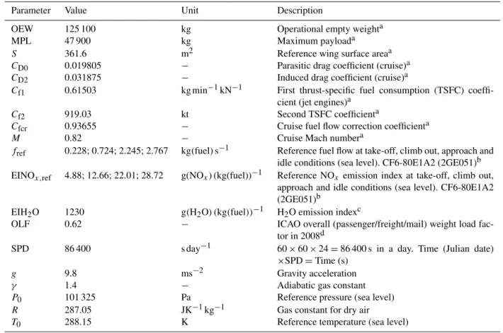
Table 1.Primary data of Airbus A330-301 aircraft and constant parameters used in AirTraf simulations.
Parameter Value Unit Description
OEW 125 100 kg Operational empty weighta
MPL 47 900 kg Maximum payloada
S 361.6 m2 Reference wing surface areaa
CD0 0.019805 − Parasitic drag coefficient (cruise)a
CD2 0.031875 − Induced drag coefficient (cruise)a
Cf1 0.61503 kg min−1kN−1 First thrust-specific fuel consumption (TSFC) coeffi-cient (jet engines)a
Cf2 919.03 kt Second TSFC coefficienta
Cfcr 0.93655 − Cruise fuel flow correction coefficienta
M 0.82 − Cruise Mach numbera
fref 0.228; 0.724; 2.245; 2.767 kg(fuel)s−1 Reference fuel flow at take-off, climb out, approach and idle conditions (sea level). CF6-80E1A2 (2GE051)b EINOx,ref 4.88; 12.66; 22.01; 28.72 g(NOx) (kg(fuel))−1 Reference NOx emission index at take-off, climb out,
approach and idle conditions (sea level). CF6-80E1A2 (2GE051)b
EIH2O 1230 g(H2O) (kg(fuel))−1 H2O emission indexc
OLF 0.62 − ICAO overall (passenger/freight/mail) weight load
fac-tor in 2008d
SPD 86 400 s day−1 60×60×24=86 400 s in a day. Time (Julian date) ×SPD=Time (s)
g 9.8 ms−2 Gravity acceleration
γ 1.4 − Adiabatic gas constant
P0 101 325 Pa Reference pressure (sea level)
R 287.05 JK−1kg−1 Gas constant for dry air
T0 288.15 K Reference temperature (sea level)
aEurocontrol (2011);bICAO (2005);cPenner et al. (1999);dAnthony (2009).
first time step of EMAC. The departure check is then per-formed at the beginning of every time step. When a flight gets to the time for departure in the time loop of EMAC, its flight status changes into “in-flight”. The time step index of EMACt is introduced here. The index is assignedt=1 to the flight at the departure time. Thereafter the flight moves to the flying process (dashed box in Fig. 1, light blue), which mainly comprises four steps (bold-black boxes in Fig. 1, light blue): flight trajectory calculation, fuel/emissions cal-culation, aircraft position calculation and gathering global emissions. The following parts of this section describe these four steps and Fig. 3a to d illustrate the respective steps.
The flight trajectory calculation linked to the aircraft rout-ing module (Fig. 1, light green) calculates a flight trajec-tory corresponding to a routing option. AirTraf will provide seven routing options: great circle (minimum flight distance), flight time (time-optimal), NOx, H2O, fuel (which might
dif-fer from H2O, if alternative fuel options can be used),
con-trail and CCFs (Frömming et al., 2013; Grewe et al., 2014b). In AirTraf (version 1.0), the great circle and the flight time routing options can currently be used. The great circle option is a basis for the other routing options and the module cal-culates a great circle by analytical formulae, assuming con-stant flight altitude. In contrast to this, for the other six
op-tions, a single-objective minimization problem is solved for the selected option by the linked flight trajectory optimiza-tion module (Fig. 1, dark green); this module comprises the Genetic Algorithm (GA, Holand, 1975; Goldberg, 1989) and finds an optimal flight trajectory including altitude changes. For example, if the flight time routing option is selected, the flight trajectory optimization is applied to all flights tak-ing into account the individual departure times. Generally, a wind-optimal route means an economically optimal flight route taking the most advantageous wind pattern into ac-count. This route minimizes total costs with respect to time, fuel and other economic costs; i.e., it has multiple objectives. AirTraf will provide the flight time and the fuel routing op-tions to investigate trade-offs (conflicting scenarios) among different routing options. With the contrail option, the best trajectory for contrail avoidance will be found. The CCFs are provided by EU FP7 project REACT4C (Reducing Emis-sions from Aviation by Changing Trajectories for the benefit of Climate, REACT4C, 2014) and estimate climate impacts due to some aviation emissions (see Sect. 1). Thus, the best trajectory for minimum CCFs will be calculated.
con-Waypoint
Flight segment
1 2
i
i+1 nwp-1 nwp
1 i
Dep. airport Arr. airport
(a)
(b)
(c)
(d)
Fcr(i)
m(i)
i+1 1
Gathering emissions: e.g. NOx emission
i i+1
i-1 Waypoint 1
One time step of EMAC
NOx(i-1) NOx(i)
t Fuel(1)
NOx(1)
H2O(1) 2 Fcr(1)
m(1)
i
Waypoint
...
...
Fcr(nwp-1)
m(nwp-1)
Lat(1) Lon(1) Alt(1) VTAS(1) Vground(1)
ETO(1)
Flight distance(nwp-1)
nwp
nwp-1
t= 1 t= 2
t= 3
Flight path corresponding to one time step of EMAC
NOx(i-2)
2 3
EINOX, a(1) EINOX, a(i) EINOX, a(nwp-1)
Lat(i) Lon(i) Alt(i) VTAS(i) Vground(i)
ETO(i)
Lat(nwp-1) Lon(nwp-1) Alt(nwp-1)
VTAS(nwp-1) Vground(nwp-1)
ETO(nwp-1)
Lat(nwp) Lon(nwp) Alt(nwp)
ETO(nwp)
ETO(1)
2.3 3.5
ETO(nwp)
nwp
1.0 posnew
posold
Dep. time
nwp-1
ETO(2) ETO(3)
{
{
{
Flight segment 1
{
i{
nwp-1{
Flight trajectory i-2
Flight trajectory
Waypoint
posnew
posold
Fcr(nwp)
m(nwp)
VTAS(nwp) Vground(nwp)
Global field (3D) EINOX, a(nwp)
...
...
...
Flight distance(i)Flight distance(1)
Fuel(i) NOx(i)
H2O(i)
Fuel(nwp-1)
NOx(nwp-1)
H2O(nwp-1)
Figure 3.Illustration of the flying process of AirTraf (dashed box in Fig. 1, light blue).(a)Flight trajectory calculation.(b)Fuel/emissions
calculation.(c)Aircraft position calculation.(d)Gathering global emissions; the fraction of NOx,icorresponding to the flight segmentiis mapped onto the nearest grid point (closed circle) relative to the (i+1)th waypoint (open circle). ETO: estimated time over;Fcr: fuel flow
of an aircraft;m: aircraft weight;t: time step index of EMAC. The detailed calculation procedures are described in Sect. 2.4.
ditions are assumed to be constant during the flight trajec-tory calculation. No weather forecasts (or weather archives) are used. Once an optimal flight trajectory is calculated, it is not re-optimized in subsequent time steps (t≥2). The detailed flight trajectory calculation methodologies for the great circle and the flight time routing options are described in Sect. 3. After the flight trajectory calculation, the trajec-tory consists of waypoints generated along the trajectrajec-tory, and flight segments (Fig. 3a). In addition, a number of flight prop-erties are available corresponding to the waypoints, flight segments and the whole trajectory, as listed in Table 2. Here, the waypoint indexiis introduced(i=1,2,···, nwp);nwpis
the number of waypoints arranged from the departure airport (i=1) to the arrival airport (i=nwp).iis also used as the flight segment index(i=1,2,···, nwp−1).
Next, fuel use, NOxand H2O emissions are calculated by
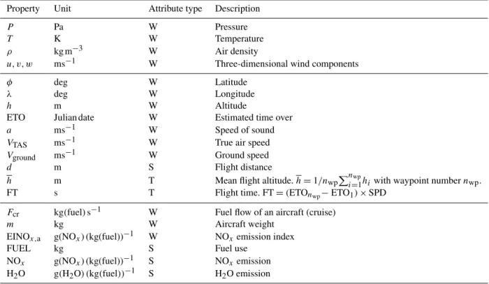
Table 2.Properties assigned to a flight trajectory. The properties of the three groups (divided by rows) are obtained from the nearest grid point of EMAC, the flight trajectory calculation (Fig. 3a), and the fuel/emissions calculation (Fig. 3b), respectively. The attribute type indicates where the values of properties are allocated. “W”, “S” and “T” stand for waypoints(i=1,2,···, nwp), flight segments(i=1,2,···, nwp−1)
and a whole flight trajectory in column 3, respectively.
Property Unit Attribute type Description
P Pa W Pressure
T K W Temperature
ρ kg m−3 W Air density
u, v, w ms−1 W Three-dimensional wind components
φ deg W Latitude
λ deg W Longitude
h m W Altitude
ETO Julian date W Estimated time over
a ms−1 W Speed of sound
VTAS ms−1 W True air speed
Vground ms−1 W Ground speed
d m S Flight distance
h m T Mean flight altitude.h=1/nwpPin=wp1hiwith waypoint numbernwp.
FT s T Flight time. FT=(ETOnwp−ETO1)×SPD
Fcr kg(fuel)s−1 W Fuel flow of an aircraft (cruise)
m kg W Aircraft weight
EINOx,a g(NOx) (kg(fuel))−1 W NOxemission index
FUEL kg S Fuel use
NOx g(NOx) (kg(fuel))−1 S NOxemission H2O g(H2O) (kg(fuel))−1 S H2O emission
The next step is to advance the aircraft positions along the flight trajectory corresponding to the time steps of EMAC (Fig. 3c). Here, aircraft position parameters posnew and
posoldare introduced to indicate the present position (at the
end of the time step) and previous position (at the begin-ning of the time step) of the aircraft along the flight trajec-tory. They are expressed by real numbers as a function of the waypoint indexi(integers), i.e., real(1,2,···, nwp). Att=1,
the aircraft is set at the first waypoint (posnew=posold=
1.0). As the time loop of EMAC progresses, the aircraft moves along the trajectory referring to the estimated time over (ETO, Table 2) (AirTraf continuously treats overnight flights with arrival on the next day). For example, Fig. 3c shows posnew=2.3 and posold=1.0 at t=2. This means
that the aircraft moves 100 % of the distance betweeni=1 andi=2, and 30 % of the distance betweeni=2 andi=3 in one time step. posnewand posoldare stored in the memory
and the aircraft continues the flight from posnew=2.3 at the
next time step. After the aircraft moves to a new position, the arrival check is performed (dashed box in Fig. 1, light blue). If posnew≥real(nwp), the flight status changes to “arrived”.
Finally, the individual aircraft’s emissions corresponding to the flight path in one time step are gathered into a global field (three-dimensional Gaussian grid). This step is applied for all flights with “in-flight” or “arrived” status. As shown in Fig. 3d, for example, the released NOx emission along a
flight segmenti(NOx,ior the fraction of it) is mapped onto the nearest grid point of the global field. For this NOx,i, the coordinates of the (i+1)th waypoint are used to find the near-est grid point. In this way, AirTraf calculates the global fields of NOx and H2O emissions, fuel use and flight distance for
output. After this step, the flight status check is performed at the end of the flying process. If the status is “arrived”, the flight quits the flying process and its status is reset to “non-flight”. Therefore, the flight status becomes either “in-flight” or “non-“in-flight” after the flying process. Once the sta-tus becomes “in-flight”, the departure check is false in sub-sequent time stepst≥2 and the aircraft moves to the new aircraft position without re-calculating the flight trajectory or fuel/emissions (Fig. 1, light blue). For simulations longer than 2 days, the same flight plan is reused: the departure time is automatically updated to the next day and the calculation procedures start from the departure check.
2.5 Fuel calculation
The methodologies of the fuel/emissions calculation mod-ule (Fig. 1, light orange) are described. Fuel use, NOx and H2O emissions are calculated along the flight trajectory
following two steps: a first rough trip fuel estimation and the second detailed fuel calculation (dashed boxes in Fig. 1, light orange). The former estimates an aircraft weight at the last waypoint (mnwp), while the latter calculates fuel use for every
flight segment and aircraft weights at any waypoint by back-ward calculation along the flight trajectory, using themnwpas
initial condition.
First, trip fuel (FUELtrip) required for a flight between a
given airport pair is roughly estimated:
FUELtrip=FBADAFT, (1)
where FT is the estimated flight time (Table 2) andFBADAis
the fuel flow. The BADA performance table provides cruise fuel flow data at specified flight altitudes for three different weights (low, nominal and high) under international standard atmosphere conditions. Hence,FBADAis calculated by inter-polating the BADA data (assuming nominal weight) to the mean altitude of the flight (h, Table 2). Next,mnwp is
esti-mated by
mnwp=OEW+MPL×OLF+rfuelFUELtrip, (2)
where OEW, MPL and OLF are given in Table 1. The last term represents the sum of an alternate fuel, reserve fuel and extra fuel. It is assumed to be 3 % of the FUELtrip (rfuel=
0.03). The burn-off fuel required to fly fromi=1 toi=nwp
and contingency fuel are assumed to be consumed during the flight and hence they are not included in mnwp. While the
3 % estimation is probably not far from reality for long-range flights, it is worth noting that typical reserve fuel quantities may amount to higher values, depending on the exact flight route. Airlines have their own fuel strategy and information about actual onboard fuel quantities is generally unavailable. Second, the burn-off fuel is calculated for every flight seg-ment and the aircraft weights are estimated at all waypoints (the contingency fuel is disregarded in AirTraf (version 1.0)). With the BADA total energy model (Revision 3.9), the rate of work done by forces acting on the aircraft is equated to the rate of increase in potential and kinetic energy:
(Thr−D)VTAS=mg
dh
dt +mVTAS
dVTAS
dt , (3)
where Thr andDare thrust and drag forces, respectively.m
is the aircraft weight,gis the gravity acceleration,h is the flight altitude and dh/dt is the rate-of-climb (or descent). For a cruise flight phase, both altitude and speed changes are negligible. Hence, dh/dt=0 as well as dVTAS/dt=0 is
as-sumed in AirTraf (version 1.0) and Eq. (3) becomes the typi-cal cruise equilibrium equation: Thri=Di at waypointi. To calculate Thri, theDi is calculated:
CL,i=
2mig
ρiVTAS2 ,iScosϕi
, (4)
CD,i=CD0+CD2CL2,i, (5)
Di= 1 2ρiV
2
TAS,iCD,iS, (6)
whereCL,i andCD,i are lift and drag coefficients, respec-tively. The performance parameters (S, CD0 and CD2) are given in Table 1,ρi is the air density (Table 2) and VTAS,i is calculated at every waypoint (Table 2). The bank angleϕi is assumed to be zero. The thrust-specific fuel consumption (TSFC)ηi and the fuel flow of the aircraftFcr,i are then cal-culated assuming a cruise flight:
ηi=Cf1
1+VTAS,i
Cf2
, (7)
Fcr,i=ηiThriCfcr, (8)
whereCf1,Cf2 andCfcrare given in Table 1. The fuel use in
theith flight segment (FUELi) is calculated as
FUELi=Fcr,i(ETOi+1−ETOi)SPD, (9)
where ETOi at theith waypoint (in Julian date) is converted into seconds by multiplying with seconds per day (SPD, Ta-ble 1). The FUELi incorporates the tail/head winds effect onVground through ETO. The relation between the FUELi
and the aircraft weight (mi) is obtained regarding theith and (i+1)th waypoints:
mi+1=mi−FUELi. (10)
Givenmnwpby Eq. (2), the fuel use for the last flight
seg-ment FUELnwp−1 and the aircraft weight at the last but one
waypointmnwp−1can be calculated. This calculation is
per-formed iteratively in reverse order from the last to first way-points using Eqs. (3) to (10). Finally, the aircraft weight at the first waypointm1is obtained.
2.6 Emission calculation
NOx and H2O emissions are calculated after the fuel
calcu-lations. NOx emission under the actual flight conditions is calculated by the DLR fuel flow method (Deidewig et al., 1996). It depends on the engine type, the power setting of the engine and atmospheric conditions. The calculation pro-cedure follows four steps. First, the reference fuel flow of an engine under sea level conditions,fref,i, is calculated from the actual fuel flow at altitude,fa,i (=Fcr,i/(number of en-gines); see Eq. 8):
fref,i=
fa,i
δtotal,ipθtotal,i
, (11)
δtotal,i=
Ptotal,i
P0
θtotal,i=
Ttotal,i
T0
, (13)
whereδtotal,i andθtotal,i are correction factors.Ptotal (in Pa)
andTtotal(in K) are the total pressure and total temperature
at the engine air intake, respectively, andP0andT0 are the
corresponding values at sea level (Table 1).Ptotal andTtotal
are calculated as
Ptotal,i=Pa,i(1+0.2M2)3.5, (14)
Ttotal,i=Ta,i(1+0.2M2), (15) wherePa,i (in Pa) andTa,i (in K) are the static pressure and temperature under actual flight conditions at the altitude hi (Table 2). Here,hi is the altitude of theith waypoint above the sea level (the geopotential altitude is used to calculatehi). The cruise Mach numberMis given in Table 1.
Second, the reference emission index under sea level con-ditions, EINOx,ref,i, is calculated using the ICAO engine emissions databank (ICAO, 2005) and the calculated refer-ence fuel flow, fref,i (Eq. 11). Four data pairs of reference fuel flows fref, and corresponding EINOx,ref, are tabulated
in the ICAO databank for a specific engine under sea level conditions. Therefore, EINOx,ref,i values, corresponding to
fref,i, are calculated by a least squares interpolation (second-order).
Third, the emission index under actual flight conditions, EINOx,a,i, is calculated from the EINOx,ref,i:
EINOx,a,i=EINOx,ref,i δtotal0.4,i θtotal3 ,i Hc,i, (16)
Hc,i=e(−19.0(qi−0.00634)), (17)
qi=10−3e(−0.0001426(hi−12,900)), (18) whereδtotal,iandθtotal,iare defined by Eqs. (12) and (13), re-spectively.Hc,iis the humidity correction factor (dimension-less number) andqi (in kg(H2O) (kg(air))−1) is the specific
humidity athi (the unit ft is used here).
Finally, NOxand H2O emissions under actual flight
con-ditions are calculated for theith flight segment using the cal-culated FUELi(Eq. 9):
NOx,i=FUELi EINOx,a,i, (19)
H2Oi =FUELi EIH2O, (20)
where the H2O emission index is EIH2O =1230
g(H2O) (kg(fuel))−1 (Penner et al., 1999). The H2O
emission is proportional to the fuel use, assuming an ideal combustion of jet fuel. The NOx and H2O emissions are
included in the flight properties (Table 2).
With regard to the reliability of the fuel/emissions calcu-lation using these methods, Schulte et al. (1997) showed a comparison of measured and calculated EINOxfor some air-craft/engine combinations (Schulte et al., 1997). The study
gave some confidence in the prediction abilities of the DLR method, although it showed that the calculated values from the DLR method underestimated the measured values on av-erage by 12 %. In Sect. 5 we verify the methods, using 1-day AirTraf simulation results. Detailed descriptions of the total energy model and the DLR fuel flow method can be found elsewhere (Eurocontrol, 2011; Deidewig et al., 1996).
3 Aircraft routing methodologies
The current aircraft routing module (Fig. 1, light green) works only with respect to the great circle and flight time routing options. These routing methodologies are described in Sects. 3.1 and 3.2. Benchmark tests are performed offline (without EMAC) to verify the accuracy of the methodolo-gies.
3.1 Great circle routing option 3.1.1 Formulation of great circles
AirTraf calculates a great circle at any arbitrary flight altitude with the great circle routing option. First, the coordinates of the waypoints are calculated. For theith and (i+1)th way-points, the central angle1σˆi (i=1,2,···, nwp−1)is
calcu-lated by the Vincenty formula (Vincenty, 1975):
1σˆi=arctan
q
(cosφi+1sin(1λi))2+(cosφisinφi+1−sinφicosφi+1cos(1λi))2
sinφisinφi+1+cosφicosφi+1cos(1λi)
, (21)
whereφi (in rad) is the latitude of theith waypoint and1λi (in rad) is the difference in longitude between theith and (i+
1)th waypoints. The Vincenty formula was set as the default method, while optionally the spherical law of cosines or the Haversine formula can be used in AirTraf to calculate1σˆ
(unshown). With Eq. (21), the great circle distance for the
ith flight segmentdiis calculated:
di=(RE+hi)1σˆi, (22)
or
di=
q
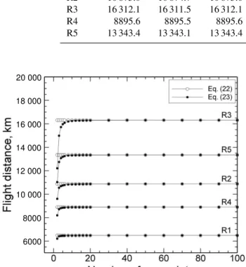
(RE+hi)2+(RE+hi+1)2−2(RE+hi)(RE+hi+1)cos(1σˆi). (23) For the great circle routing option, flight altitudes at all waypoints are set ashi = constant fori=1,2,···, nwp(hi is used in kilometers in Eqs. 22 and 23) and either Eq. (22) or (23) is used to calculatedi. Equation (22) calculatesdi by an arc and hence the great circle distance between airports, i.e., Pnwp−1
i=1 di, is independent ofnwp. On the other hand,
Eq. (23) calculatesdiby linear interpolation in polar coordi-nates. In that case,Pnwp−1
i=1 di depends onnwp; the sum
be-comes close to that calculated from Eq. (22) with increasing
Longitude
Latitude
90˚ S 60˚ S 30˚ S 0˚ 30˚ N 60˚ N 90˚ N
180˚ 120˚ W 60˚ W 0˚ 60˚ E 120˚ E 180˚
R1 R2
R3
R4 MUC
JFK HND
SYD R5
R2
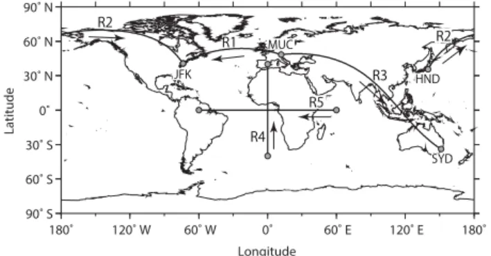
Figure 4.Five representative routes for the great circle benchmark
test. The details of locations are listed in Table 3.
are compared to those with other routing options, Eq. (23) should be used for the comparison with the samenwp. In
ad-dition, Eq. (23) is used for the flight trajectory optimization (see Sect. 3.2), because it is necessary to calculatedi includ-ing altitude changes.
Next, the true air speedVTASand the ground speedVground
at theith waypoint are calculated:
VTAS,i=Mai=M
p
γ RTi, (24)
Vground,i=VTAS,i+Vwind,i, (25)
where M is the Mach number,γ is the adiabatic gas con-stant andRis the gas constant for dry air (Table 1). Temper-atureTiand three-dimensional wind components(ui, vi, wi) of the ith waypoint are available from the EMAC model fields at t=1; the local speed of sound ai is then calcu-lated (Table 2). The flight direction is calcucalcu-lated for every flight segment by using the three-dimensional coordinates of the ith and (i+1)th waypoints. Thereafter, VTAS,i,Vwind,i and Vground,i (scalar values) corresponding to the flight di-rection are calculated. As shown in Eq. (25), the influence of tail/head winds on ground speed is considered. In AirTraf,
M was set constant as default. It is also possible to perform AirTraf simulations with different options, such asVTAS,i= constant andVwind,i=0. Finally, ETOi (in Julian date) and FT (in s) are calculated as
ETOi=ETOi−1+
di−1 Vground,i−1×SPD
(i=2,3,···, nwp), (26)
FT=(ETOnwp−ETO1)×SPD, (27)
where ETO1is the departure time of the flight and ETOi in-corporates the influence of tail/head winds on the flight. 3.1.2 Benchmark test on great circle calculations A benchmark test of the great circle routing option was performed to confirm the accuracy of the great circle dis-tance calculation. Great circles were calculated for five rep-resentative routes without EMAC (offline). Table 3 shows the information for the five routes (the locations are shown
in Fig. 4). The characteristics of the routes were as fol-lows: R1 consisted of an airport pair in the Northern Hemi-sphere (MUC-JFK) and the difference in longitude between them was1λairport<180◦; R2 consisted of an airport pair in
the Northern Hemisphere (HND-JFK) with1λairport>180◦
(discontinuous longitude values due to the definition of the longitude range[−180,180]); R3 consisted of an airport pair in the Northern and Southern Hemisphere (MUC-SYD); R4 was a special route, where1λairport=0◦and the difference
in latitude was1φairport6=0◦; and R5 was another special
route with1λairport6=0◦ and1φairport=0◦. Other
calcula-tion condicalcula-tions were set as follows:M=0.82,hi=0,ai= 304.5 ms−1andVTAS,i=Vground,i=249.7 ms−1(under no-wind conditions, i.e.,Vwind,i=0) fori=1,2,···, nwp. The
great circle distances Pnwp−1
i=1 di were each calculated by Eqs. (22) and (23), and were compared to that calculated with MTS. In addition, the sensitivity of the great circle distance with respect tonwpwas analyzed varyingnwp in the range
[2,100].
Table 4 shows the calculated great circle distances by Eqs. (22) and (23) and MTS. The columns 5 to 7 show the difference in the distance among them (see the caption of Table 4 for more details). The results showed that both
1deq23,eq22 and 1deq23,MTS varied between −0.0036 and −0.0005 %, while1deq22,MTS showed 0.0 %. The great
cir-cle distances calculated by Eqs. (22) and (23) were accurate to−0.004 %, and hence this routing option works properly. Figure 5 shows the result of the sensitivity analysis ofnwpon
the great circle distance. The results show that the distance calculated by Eq. (22) (open circle) has no dependence on
nwpas noted in Sect. 3.1.1, whereas that by Eq. (23) (closed
circle) depends onnwp and converged with increasingnwp: the accuracy of the results by Eq. (23) decreased when using fewernwp. For nwp≥20, the results of Eqs. (22) and (23)
were almost the same. Therefore,nwp≥20 is practically
de-sired for the use of Eq. (23). 3.2 Flight time routing option
3.2.1 Overview of the genetic algorithm
Table 3.Information for the five representative routes of the great circle benchmark test.
Route Departure airport Latitude Longitude Arrival airport Latitude Longitude
R1 Munich (MUC) 48.35◦N 11.79◦E New York (JFK) 40.64◦N 73.78◦W R2 Tokyo Haneda (HND) 35.55◦N 139.78◦E New York (JFK) 40.64◦N 73.78◦W R3 Munich (MUC) 48.35◦N 11.79◦E Sydney (SYD) 33.95◦S 151.18◦E
R4 – 40.0◦S 0 – 40.0◦N 0
R5 – 0 60.0◦E – 0 60.0◦W
Table 4.Great circle distance (d) of the five representative routes calculated with different calculation methods. Column 2 (deq22) corresponds
to the result calculated by Eq. (22); column 3 (deq23) corresponds to the result calculated by Eq. (23) withnwp=100; and column 4 (dMTS)
shows the result calculated with the Movable Type scripts (MTS), using the Haversine formula with a spherical Earth radius ofRE=6371 km.
In columns 5 to 7:1deq23,eq22=(deq23deq22−deq22)×100,1deq23,MTS=(deq23dMTS−dMTS)×100, and1deq22,MTS=(deq22dMTS−dMTS)×100.
Route deq22, km deq23, km dMTS, km 1deq23,eq22, % 1deq23,MTS, % 1deq22,MTS, %
R1 6481.1 6481.0 6481.1 −0.0005 −0.0005 0.0000
R2 10 875.0 10 874.7 10 875.0 −0.0028 −0.0028 0.0000
R3 16 312.1 16 311.5 16 312.1 −0.0036 −0.0036 0.0000
R4 8895.6 8895.5 8895.6 −0.0008 −0.0008 0.0000
R5 13 343.4 13 343.1 13 343.4 −0.0019 −0.0019 0.0000
20 000
18 000
16 000
14 000
12 000
10 000
8000
6000
Figure 5.Comparison of the flight distance for the five
representa-tive routes.◦: great circle distance calculated by Eq. (22);•: great circle distance calculated by Eq. (23).
is that GA requires neither the computation of derivatives or gradients of functions, nor the continuity of functions. There-fore, various evaluation functions (called objective functions) can easily be adapted to GA. As for the working principle of GA, a random initialpopulationis created and thepopulation
evolves overgenerationsto adapt to an environment by the genetic operators: evaluation, selection, crossover and mu-tation. When this biological evolutionary concept is applied for design optimizations,fitness, individuals and genes cor-respond to an objective function, solutions and design
vari-ables, respectively. A solution found in GA is called an op-timal solution, whereas a solution with the theoretical opti-mum of the objective function is called the true-optimal solu-tion. If GA works properly, it is expected that the optimal so-lution will converge to the true-optimal soso-lution. On the other hand, the main disadvantage of GA is that GA is computa-tionally expensive. The flight trajectory optimization is ap-plied for all flights and therefore a user has to choose appro-priate GA parameter settings to reduce computational costs (or find a compromise for the settings, which sometimes de-pend on the computing environment).
3.2.2 Formulation of flight trajectory optimization The flight trajectory optimization is described focusing on geometry definitions of the flight trajectory, the definition of the objective function and the genetic operators. There ex-ist a number of selection, crossover and mutation operators in ARMOGA. Therefore, the genetic operators employed in this study are described here.
A solution x (the term is used interchangeably with
flight trajectory) is a vector of ndv design variables: x= (x1, x2,···, xndv)
T. Using the design variable index j (j = 1,2,···, ndv), the jth design variable varies in lower/upper
0 2000 4000 6000 8000 10 000 12 000
Longitude
Latitude
Altitude, m
Ground
20˚ N 40˚ N 60˚ N
90˚ W 60˚ W 30˚ W 0˚ 30˚ E
JFK
MUC
(x1, x2)
(x3, x4)
(x5, x6)
x7
x8
x9
x10
x11
hu= FL410
hl= FL290
∆λairport
Flight direction
0.1∆λairport
0.3∆λairport
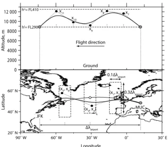
Figure 6. Geometry definition of flight trajectory in the
verti-cal cross section (top) and projection on the Earth (bottom). The bold solid line indicates a trajectory from MUC to JFK.•: control points determined by design variablesx=(x1, x2,···, x11)T. The lower/upper bounds of the 11 design variables are shown in Table 6. Bottom: the dashed boxes show rectangular domains of three con-trol points.3: central points of the domains are calculated on the great circle (thin solid line), which divide the1λairport into four
equal parts. Top: the dashed lines show the lower/upper variable bounds in altitude. “FL290” stands for a flight level at 29 000 ft. Longitude coordinates forx7, x8,···, x11are pre-calculated; the
co-ordinates divide the1λairportinto six equal parts.
fixed (the coordinates of MUC and JFK are shown in Ta-ble 5).
Six design variablesxj(j=1,2,···,6)were used for loca-tion, as shown in Fig. 6 (bottom).x1,x3andx5indicate
lon-gitudes, whilex2,x4andx6indicate latitudes. To create three
rectangular domains for the design variables (dashed boxes), central points of the domains (diamond symbols) were cal-culated. The points are located on the great circle, divid-ing the longitude distance between MUC and JFK (1λairport)
into four equal parts. After that, the three domains centered around the central points were created. The domain size was set to 0.1×1λairport (short-side) and 0.3×1λairport
(long-side). This procedure calculates the lower/upper bounds of the six design variables, i.e., [xjl, xju] (j=1,2,···,6), and Table 6 lists these values. GA provided the values forx1tox6
within the respective bounds (i.e., the values were generated within the rectangular domains) and the coordinates of the three CPs were determined: CP1 (x1,x2), CP2 (x3,x4) and
CP3 (x5,x6). A flight trajectory is represented by a B-spline
curve (third-order) with the three CPs as locations (bold solid line, Fig. 6 bottom), and then any arbitrary number of way-points is generated along the trajectory. To generate the same number of waypoints between the CPs,nwpwas calculated as
mod(nwp−1, nCPloc+1)=0, where the number of CPs was
nCPloc=3.
For the altitude direction, five design variables xj(j= 7,8,···,11)were used (Fig. 6, top). Herex7tox11 indicate
altitude values. With the lowerhl and the upperhuvariable bound parameters, the bounds of the five design variables were determined byxjl =hlandxju=huforj =7,8,···,11. In this study,hl=FL290 andhu=FL410, as listed in Ta-ble 6 (“FL290” stands for a flight level at 29 000 ft). These altitudes correspond to a general cruise flight altitude range of commercial aircraft (Sridhar et al., 2013). GA provided the values ofx7tox11in[FL290, FL410]and the coordinates of
the five CPs were determined: CP4 (x7), CP5 (x8), CP6 (x9),
CP7 (x10) and CP8 (x11). Note that these values vary freely between FL290 and FL410 to explore widely the possibility of minimizing climate impact by aircraft routing. The longi-tude coordinates of the five CPs were pre-calculated to divide the1λairportinto six equal parts. The altitudes of the airports
were fixed athl(=FL290). A flight trajectory is also repre-sented by a B-spline curve (third-order) with the five CPs in the vertical cross section (bold solid line, Fig. 6 top) and then waypoints are generated along the trajectory in such a way that the longitude of the waypoints is the same as that for the flight trajectory projected on the Earth.
GA starts its search with a random set of solutions (
pop-ulation approach). The initial population operator (Fig. 1,
dark green) provides initial values of the 11 design variables at random within the lower/upper bounds described above, thereby creating solutions. The operator createsnpdifferent solutions (wherenpis thepopulationsize). To evaluate the
solutions, the objective functionf was calculated for each of the solutions by summing the flight time over all flight seg-ments (Fig. 1, dark green). The single-objective optimization problem on the flight time can be written as follows:
Minimize f =
nwp−1
P
i=1 di
Vground,i Subject to xjl ≤xj≤xju, j=1,2,···, ndv
, (28)
wherendv=11,di andVground,i are calculated by Eqs. (23) and (25), respectively (VTAS,i andVwind,i are calculated as described in Sect. 3.1.1). No constraint function is used in AirTraf (version 1.0).
Good solutions are identified in thepopulationby Fonseca and Fleming’s Pareto ranking method (Fonseca and Fleming, 1993), although the single-objective optimization is solved here. Arankof a solution was assigned proportionally to the number of solutions that dominate it, and afitness value of a solution was computed by 1/rank (nofitnesssharing was used). A solution with a higherfitnessvalue (i.e., a smaller
rank value) has a higher probability of being copied into
amating pool. The stochastic universal sampling selection
(Baker, 1985) makes duplicates of good solutions in the
mat-ing poolat the expense of bad solutions based on cumulative
Table 5.Calculation conditions for the benchmark test on flight trajectory optimizations.
Parameter Description
Objective function Minimize flight time
Design variable,ndv 11 (6 locations and 5 altitudes) Number of waypoints,nwp 101
Departure airport MUC (lat.=48.35◦N, lon.=11.79◦E, alt.=FL290) Arrival airport JFK (lat.=40.64◦N, lon.=73.78◦W, alt.=FL290) VTAS,Vground 898.8 km h−1(constant)
Vwind 0 (no-wind)
Optimizer Real-coded GA∗
Population size,np 10,20, . . .,100
Number of generations,ng 10,20, . . .,100
Selection Stochastic universal sampling Crossover Blend crossover BLX-0.2 (α=0.2)
Mutation Revised polynomial mutation (rm=0.1;ηm=5.0)
∗Sasaki et al. (2002) and Sasaki and Obayashi (2004).
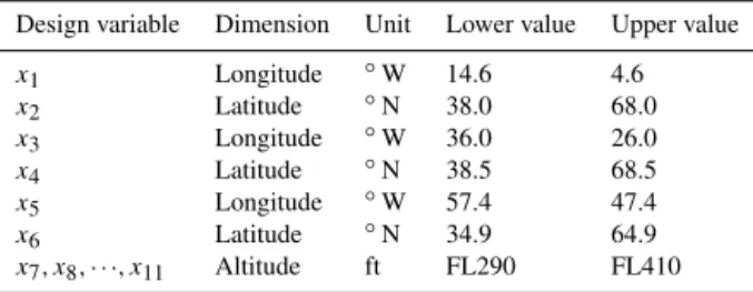
Table 6.Lower/upper bounds of the 11 design variables.
Design variable Dimension Unit Lower value Upper value
x1 Longitude ◦W 14.6 4.6
x2 Latitude ◦N 38.0 68.0
x3 Longitude ◦W 36.0 26.0
x4 Latitude ◦N 38.5 68.5
x5 Longitude ◦W 57.4 47.4
x6 Latitude ◦N 34.9 64.9
x7, x8,···, x11 Altitude ft FL290 FL410
To create a new solution, the Blend crossover (BLX-α) op-erator (Eshelman, 1993) was applied to thepopulationin the
mating pool. Two solutions (parent solutions) were picked
from themating poolat random and the operator created two new solutions (child solutions):
xj,c1=γ xj,p1+(1−γ )xj,p2 xj,c2=(1−γ )xj,p1+γ xj,p2
, (29)
withγ=(1+2α)u1−αandj varies in[1, ndv](ndv=11). xj,c1 andxj,c2 denote the jth design variable of the child
solutions, andxj,p1andxj,p2denote thejth design variables
of the parent solutions (the mated pair of the oldgeneration).
αis a user-specified crossover parameter andu1is a random
number between zero and one.
Thereafter, the mutation operator added a disturbance to the child solutions by the revised polynomial mutation op-erator (Deb and Agrawal, 1999) with a mutation raterm. A
polynomial probability distribution was used and the mutated design variable was created. The parameterδq is first calcu-lated as
δq=
(
[2u2+(1−2u2)(1−δ)ηm+1]
1
ηm+1−1, ifu2≤0.5,
1− [2(1−u2)+2(u2−0.5)(1−δ)ηm+1]
1
ηm+1, ifu
2>0.5,
(30) whereδ=min[(xj,c−xjl), (xju−xj,c)]/(xju−xjl). Thejth de-sign variable varies in[xjl, xju].u2 is a random number
be-tween zero and one, andηmis an external parameter
control-ling the shape of the probability distribution. The mutated design variable (mutated child solution)xj,mc is calculated
as follows:
xj,mc=xj,c+δq(xju−xjl), j=1,2,···, ndv. (31) Using the genetic operators above, it is expected that the
populationof solutions will be improved and a new and
bet-terpopulationcreated in subsequentgenerations. When the
evolution is computed for a fixed number ofgenerationsng,
GA quits the optimization and an optimal solution showing the bestf of the whole generation is output. The optimal solution has the superior combination of the 11 design vari-ablesx=(x1, x2,···, x11)T to minimizef. The flight
prop-erties of the optimal solution are also available (ETO,h, FT, etc., listed in the first and second groups (divided by rows) of Table 2). The flight trajectory optimization methodology de-scribed here could be applied to any routing option (except for the great circle routing option). In that case, the objec-tive functionf given by Eq. (28) needs to be reformulated corresponding to the selected routing option.
3.2.3 Benchmark test on flight trajectory optimization with flight time routing option
To quantify the performance of GA, there is a need to choose an appropriate benchmark test of the flight trajectory opti-mization, where the true-optimal solution ftrue of the test is known. Here, the single-objective optimization for mini-mization of flight time from MUC to JFK was solved with-out EMAC (offline); that is, the optimization problem defined in Sect. 3.2.2 was solved. Calculation conditions for the test are summarized in Table 5.Vwindwas set to 0 km h−1
(no-wind conditions);VTASandVgroundwere set to 898.8 km h−1
(constant). Hence,ftrueequals the flight time along the great
Table 7.Setup for AirTraf 1-day simulations.
Parameter Routing option
Great circle Flight time
ECHAM5 resolution T42L31ECMWF (2.8◦by 2.8◦)
Duration of simulation 1–2 January 1978, 00:00:00 UTC
Time step of EMAC 12 min
Flight plan 103 trans-Atlantic flights (eastbound 52/westbound 51)∗
Aircraft type A330-301
Engine type CF6-80E1A2, 2GE051 (with 1862M39 combustor)
Flight altitude changes Fixed FL290, FL330, FL370, FL410 [FL290, FL410]
Mach number 0.82
Wind effect Three-dimensional components (u,v,w)
Number of waypoints,nwp 101
Optimization − Minimize flight time
Design variable,ndv − 11 (6 locations and 5 altitudes)
Population size,np − 100
Number of generations,ng − 100
Selection − Stochastic universal sampling
Crossover − Blend crossover BLX-0.2 (α=0.2)
Mutation − Revised polynomial mutation (rm=0.1;ηm=5.0)
∗REACT4C (2014).
the range of[FL290, FL410]):ftrue=25 994.0 s calculated
by Eq. (23) with hi=FL290 for i=1,2,···,101. Ten in-dependent GA simulations from different initialpopulations
were performed for each combination ofnp(10,20,···,100)
andng(10,20,···,100); i.e., a total of 1000 independent GA
simulations were performed. 3.2.4 Optimization results
The influence of the populationsize npand the number of
generationsngon the convergence properties of GA was
ex-amined. Figure 7 shows the optimal solutions varying withng
for a number of fixednp. The results confirmed that the
opti-mal solutions come sufficiently close toftruewith increasing np andng. The optimal solution showing the closest flight
time toftruewas obtained fornp=100 andng=100. This
solution is called best solution in this study and its flight time wasfbest=25 996.6 s. The difference in flight time between
thefbestandftruewas1f <3.0 s (less than 0.01 %).
To confirm the diversity of GA optimization, we focus on the optimization yielding the best solution (np=100 and ng=100). Figure 8 shows all the solutions explored by GA. It is clear that GA explored diverse solutions from MUC to JFK including altitude changes and found the best solution. As shown in Fig. 8, the best solution (red line) overlapped with the true-optimal solution, i.e., the great circle at FL290 (dashed line, black). To investigate the difference between the solutions, the comparisons of trajectories for the best so-lution and the true-optimal soso-lution in the vertical cross sec-tion are plotted in Fig. 9. The maximum difference in altitude is less than 1 m. Therefore, GA is adequate for finding an
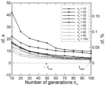
op-Figure 7.Optimal solutions varying with thepopulationsizenpand
the number ofgenerationsng.1f means the difference in flight
time between the optimal solutionf and the true-optimal solution ftrue(=25 994.0 s). The1f (in %) is calculated as(1f/ftrue)×
100. The flight time of the best solution isfbest=25 996.6 s (for np=100 andng=100,1f <3.0 s (less than 0.01 %)).
timal solution with sufficient accuracy (in a strict sense, this conclusion is confined to the benchmark test).
3.2.5 Dependence of initial populations
Figure 8. Ten-thousand explored trajectories (solid line, black) from MUC to JFK in the vertical cross section (top) and projection on the Earth (bottom). Thepopulationsizenpis 100 and the number
ofgenerationsngis 100. The best solution (red line) overlaps with
the true-optimal solution (dashed line, black), i.e., the great circle at FL290. The flight time of the best solution is 25 996.6 s, while that of the true-optimal solution is 25 994.0 s.
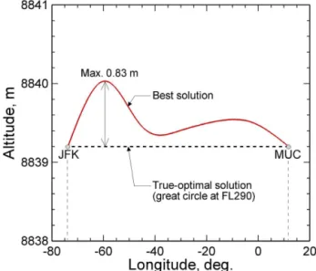
Figure 9.Trajectories for the best solution (red line) and the
true-optimal solution (dashed line, black). This shows the enlarged draw-ing of Fig. 8 (top). The maximum difference in altitude is 0.83 m.
of objective function evaluations(=np×ng)for the 10
in-dependent GA simulations from different initial populations withnp=100 andng=100. Figure 10 shows that the 10
so-lutions converged in earlygenerationsand gradually contin-ued to converge toftruewith an increasing number of
func-tion evaluafunc-tions. The convergence behavior is similar among the 10 simulations, regardless of the initial population.
Ta-Figure 10.Flight time vs. number of function evaluations (=np×
ng), including the enlarged drawing in the early 1000 evaluations.
Thepopulationsizenpis 100 and the number ofgenerationsngis
100.1fmeans the difference in flight time between the solutionf and the true-optimal solutionftrue(=25 994.0 s). The1f (in %)
is calculated as(1f/ftrue)×100. The solution shown as red line
corresponds to the best solution in Figs. 7 to 9. Table S1 summarizes the 10 optimal solutions in detail.
ble S1 in the Supplement shows a summary of the 10 optimal solutions. As indicated in Table S1, the value of the objective functionf (flight time) is slightly different.1f (=f−ftrue)
ranged from 2.5 to 3.7 s, which is approximately 0.01 % of
ftrue. In addition, the mean value of the 10 objective func-tions was1f=2.9 s (0.01 % offtrue) and the standard
devi-ation wass1f =0.4 s (0.001 % offtrue). Therefore, the
vari-ation in the objective function with different initial popula-tions is small.
3.2.6 Population and generation sizing
With increasednpandng, GA tends to find an improved
so-lution. It is important to note that the required size ofnpand ngis problem-dependent. However, following a simple initial
guess fornpandngis a good starting point for their sizing.
The influences ofnpandng on the accuracy of GA
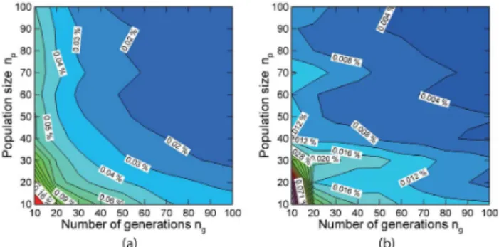
opti-mizations and on the variation in the optimal solution due to different initial populations were analyzed. Figure 11 shows the1f ands1f for all the combinations ofnp andng. The
results confirm that1f ands1f decrease with an increase in
npandng. That is, the optimal solution converges to the
true-optimal solution (the accuracy increases) and the variation in the optimal solution due to different initial populations de-creases (the dependency dede-creases).
combina-Figure 11.Variation of the mean value of the difference in flight time between the true-optimal solution (ftrue=25 994.0 s) and the
optimal solution1f (a), and the standard deviations of1f (s1f,
b) are shown varying with thepopulationsizenpand the number of generationsng. The variation was calculated by 10 independent GA
simulations from different initialpopulationsfor each combination ofnpandng: in total, 1000 independent simulations. On the1fand s1f:1f=1n
Pn
i=11fi,s1f=
q 1
n−1 Pn
i=1(1fi−1f )2, where n=10.1fands1f (in %) relative to the true-optimal solution are calculated as(1f /ftrue)×100 and(s1f/ftrue)×100, respectively.
tions of np andng with respect to the number of function
evaluations. The symbols and error bars in the figure cor-respond to1f ands1f, respectively (Table S2 in the Sup-plement lists these values). The results showed that there is a trade-off between the accuracy of GA optimizations and the number of function evaluations (i.e., computing time). The figure also shows the power function (red line) fitted to the results by using the standard least squares algorithm (see the caption in Fig. 12 for more details). The enlarged drawing in Fig. 12 shows that if one selects the number of function evaluations(=np×ng)of 800, the large reduction of computational costs of 92 % can be achieved, keeping1f
less than 0.05 % (s1f ≈0.02 %), compared to the optimal solution obtained by 10 000 function evaluations (np=100
andng=100). Fornp×ng=800, one can select any
com-bination of np andng:np=10 and ng=80,np=20 and ng=40, etc. A user makes his/her own choice onnpandng
by referring to the values of1f ands1f shown in Fig. 12. Similarly, a reduction of 97 % can be achieved, keeping1f
less than 0.1 % (s1f ≈0.04 %). Therefore, computational costs can be reduced drastically by selectingnpandngfor
different purposes.
4 Demonstration of a 1-day AirTraf simulation
The aircraft routing methodologies corresponding to the great circle and flight time routing options were verified in Sect. 3. Here, 1-day AirTraf simulations were performed in EMAC (online) with the respective routing options for demonstration.
Figure 12.Chart for finding the appropriate number of function
evaluations (=np×ng), including the enlarged drawing in the early
1500 evaluations. The symbols with error bars correspond to1f± s1f (in %); their definitions are given in the caption in Fig. 11. The fitted curve (power function, red line) to1f isy=e0.92x−0.59, wherexare the function evaluations andyis1f(in %);R2=0.89. The fitted curve tos1f is calculated similarly:y=e0.67x−0.73, whereR2=0.71 (unshown).
4.1 Simulation setup
We focus on the trans-Atlantic region for the demonstration, because the optimization potential is possibly large for this region. Table 7 lists the setup for the 1-day simulations. The simulations were performed for 1 typical winter day in the T42L31ECMWF resolution. The weather situation on that day showed a typical weather pattern for winter character-ized by westerly jet streams in the North Atlantic region. The number of trans-Atlantic flights in the region was 103 (52 eastbound flights and 51 westbound flights). We assumed that all flights were operated by A330-301 aircraft with CF6-80E1A2 (2GE051) engines. Thus, the data shown in Ta-ble 1 were used. Four 1-day simulations were separately per-formed for the great circle routing option at fixed altitudes FL290, FL330, FL370 and FL410 (see Sect. 3.1.1). In addi-tion, a single 1-day simulation was performed for the flight time routing option, including altitude changes in the range of[FL290, FL410](see Sect. 3.2.2). For the two options, the Mach number was set toM=0.82 and therefore the values ofVTASandVgroundwere different at every waypoint (Eqs. 24
and 25). The number of waypoints was set tonwp=101. As
described in Sect. 3.1.1, the flight distance was calculated by Eq. (23) for the two routing options. The optimization param-eters were set as follows:np=100,ng=100 and other GA
T able 8. Information for the trajec tories of the three selected airport pairs; the y were extracted from the 1-day AirT raf simulations. Columns 7 to 11 sho w the obtained flight times for the flight time and great circle routing options. GC FL290: great circle at 29 000 ft. T ype Departure airport Arri val airport Flight direction Departure time, UTC Mean flight altitude h ,m (in ft) Flight time FT , s T ime-optimal GC FL290 GC FL330 GC FL370 GC FL410 I Ne w Y ork (JFK) Munich (MUC) Eastbound 01:30:00 8841 (29 005) 23 986.2 24 100.1 24 472.1 24 772.6 24 931.9 Munich (MUC) Ne w Y ork (JFK) W estbound 14:27:00 8839 (29 000) 28 429.0 29 417.3 29 856.7 29 899.0 29 538.5 II Minneapolis (MSP) Amsterdam (AM S) Eastbound 21:35:00 8839 (29 000) 25 335.6 25 958.4 25 957.9 25 989.3 26 043.9 Amsterdam (AMS) Minneapolis (MSP) W estbound 12:50:00 10 002 (32 815) 28 869.5 29 117.0 29 211.7 29 292.6 29 219.1 III Seattle (SEA) Amsterdam (AM S) Eastbound 21:05:00 10 829 (35 527) 31 784.6 31 962.9 31 943.5 31 841.9 31 825.4 Amsterdam (AMS) Seattle (SEA) W estbound 12:30:00 9311 (30 546) 33 010.5 33 026.2 33 230.5 33 342.6 33 354.1
The 1-day simulation was parallelized on four PEs of Fu-jitsu Esprimo P900 (Intel Core i5-2500 CPU with 3.30 GHz; 4 GB of memory; peak performance of 105.6×4 GFLOPS) at the Institute of Atmospheric Physics, German Aerospace Center. The 1-day simulation required approximately 15 min for the great circle routing option, while it took approxi-mately 20 h for the flight time routing option. Most of the computational time is consumed by the trajectory optimiza-tions. Therefore this time can be reduced by choosing prop-erly all GA parameters, using more PEs, or decreasingnpand ng. As discussed in Sect. 3.2.6, a large reduction in
comput-ing time of roughly 90 % can be achieved by uscomput-ing a small
npandngwith still sufficient accuracy of the optimizations.
4.2 Optimal solutions for selected airport pairs
The 1-day simulation results for the flight time routing op-tion confirmed that the optimized flight trajectories showed a large altitude variation. To give an overview of the opti-mizations, we classified those optimized flight trajectories according to their altitude changes into three categories. Type I: eastbound and westbound time-optimal flight trajec-tories showed little altitude changes; Type II: the eastbound time-optimal flight trajectory showed little altitude changes, while the westbound time-optimal flight trajectory showed distinct altitude changes; and Type III: eastbound and west-bound time-optimal flight trajectories showed distinct alti-tude changes. We have selected three airport pairs of each type and Table 8 shows the details of them. Here, we mainly discuss the selected solutions of Type II, which were east-bound and westeast-bound flights between Minneapolis (MSP) and Amsterdam (AMS).
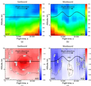
We examined first the optimal flight trajectories between MSP and AMS. Figure 13 shows all trajectories explored by GA (black lines) and the time-optimal flight trajectories for eastbound and westbound flights (red and blue lines). Fig-ure 13a and b show that GA explored diverse trajectories properly considering altitude changes in the range of[FL290, FL410]. Similar results were obtained for the selected so-lutions of Types I and III, as shown in Figs. S1 and S2 in the Supplement. In addition, the eastbound time-optimal flight trajectory was located at FL290, while that for west-bound flights showed large altitude changes; i.e., it climbed, descended, climbed and then descended again. The mean flight altitudes of these trajectories were h=8839 m and
h=10 002 m. These time-optimal flight trajectories were compared to the prevailing wind fields. To calculate tail/head winds in the eastern and western directions, the major wind component is shown in Fig. 14. The contours represent the zonal wind speed (u); black arrows show the wind speed (√u2+v2) and direction at the departure time at h.