www.biogeosciences.net/7/3707/2010/ doi:10.5194/bg-7-3707-2010
© Author(s) 2010. CC Attribution 3.0 License.
Biogeosciences
Deciphering the components of regional net ecosystem fluxes
following a bottom-up approach for the Iberian Peninsula
N. Carvalhais1,2, M. Reichstein2, G. J. Collatz3, M. D. Mahecha2, M. Migliavacca4, C. S. R. Neigh5, E. Tomelleri2, A. A. Benali1, D. Papale6, and J. Seixas1
1Departamento de Ciˆencias e Engenharia do Ambiente, DCEA, Faculdade de Ciˆencias e Tecnologia, FCT, Universidade Nova de Lisboa, 2829-516 Caparica, Portugal
2Max-Planck-Institut f¨ur Biogeochemie, P.O. Box 10 01 64, 07701 Jena, Germany 3NASA Goddard Space Flight Center, Greenbelt, Code 614.4, Greenbelt, MD 20771, USA
4European Commission – Directorate General Joint Research Centre, Institute for Environment and Sustainability, Climate Change Unit, 21027 Ispra (VA), Italy
5NASA Postdoctoral Program Fellow, Goddard Space Flight Center, Greenbelt MD 20771, USA
6Dipartimento di Scienze dell’Ambiente Forestale e delle sue Risorse, DISAFRI, Universit´a degli Studi della Tuscia, Via Camillo de Lellis, snc-01100, Viterbo, Italy
Received: 8 March 2010 – Published in Biogeosciences Discuss.: 22 June 2010
Revised: 30 October 2010 – Accepted: 2 November 2010 – Published: 18 November 2010
Abstract.Quantification of ecosystem carbon pools is a fun-damental requirement for estimating carbon fluxes and for addressing the dynamics and responses of the terrestrial car-bon cycle to environmental drivers. The initial estimates of carbon pools in terrestrial carbon cycle models often rely on the ecosystem steady state assumption, leading to initial equilibrium conditions. In this study, we investigate how trends and inter-annual variability of net ecosystem fluxes are affected by initial non-steady state conditions. Further, we examine how modeled ecosystem responses induced ex-clusively by the model drivers can be separated from the ini-tial conditions. For this, the Carnegie-Ames-Stanford Ap-proach (CASA) model is optimized at set of European eddy covariance sites, which support the parameterization of re-gional simulations of ecosystem fluxes for the Iberian Penin-sula, between 1982 and 2006.
The presented analysis stands on a credible model perfor-mance for a set of sites, that represent generally well the plant functional types and selected descriptors of climate and phenology present in the Iberian region – except for a lim-ited Northwestern area. The effects of initial conditions on inter-annual variability and on trends, results mostly from the recovery of pools to equilibrium conditions; which control most of the inter-annual variability (IAV) and both the
mag-Correspondence to:N. Carvalhais ([email protected])
nitude and sign of most of the trends. However, by removing the time series of pure model recovery from the time series of the overall fluxes, we are able to retrieve estimates of inter-annual variability and trends in net ecosystem fluxes that are quasi-independent from the initial conditions. This approach reduced the sensitivity of the net fluxes to initial conditions from 47% and 174% to−3% and 7%, for strong initial sink and source conditions, respectively.
With the aim to identify and improve understanding of the component fluxes that drive the observed trends, the net ecosystem production (NEP) trends are decomposed into net primary production (NPP) and heterotrophic respiration (RH) trends. The majority (∼97%) of the positive trends in NEP is observed in regions where both NPP andRHfluxes show significant increases, although the magnitude of NPP trends is higher. Analogously,∼83% of the negative trends in NEP
are also associated with negative trends in NPP. The spatial patterns of NPP trends are mainly explained by the trends infAPAR (r=0.79) and are only marginally explained by trends in temperature and water stress scalars (r=0.10 and r=0.25, respectively). Further, we observe the signifi-cant role of substrate availability (r=0.25) and temperature (r=0.23) in explaining the spatial patterns of trends inRH. These results highlight the role of primary production in driv-ing ecosystem fluxes.
need to decompose the ecosystem fluxes into its components and drivers for more mechanistic interpretations of modeling results. We expect that our results are not only specific for the CASA model since it incorporates concepts of ecosys-tem functioning and modeling assumptions common to bio-geochemical models. A direct implication of these results is the ability of this approach to detect climate and phenology induced trends regardless of the initial conditions.
1 Introduction
The quantification of terrestrial net ecosystem fluxes is of significant importance to the understanding of the global carbon cycle (e.g., Heimann and Reichstein, 2008) and has been the subject of active research (e.g., Ciais et al., 2000; Piao et al., 2009b). In this regard, model-data synthesis ap-proaches have focused on the improvement of ecosystem flux estimates through model structure development (e.g., Richardson et al., 2006), estimation of parameters (e.g., Knorr and Kattge, 2005) and initial conditions (e.g., Braswell et al., 2005; Carvalhais et al., 2008), adjustments in state ables (e.g., Jones et al., 2004) and sensitivity to forcing vari-ables (e.g., Abramowitz et al., 2008). The wide assessment of uncertainties in the different modeling components can fur-ther be integrated in bottom-up approaches and should be a robust indicator of the overall methodological uncertainties (Raupach et al., 2005). The further integration of different models in ensemble approaches establishes the boundaries of prognostic scenarios for future climate conditions (e.g., Sitch et al., 2008; van den Berge, 2010).
In process-based biogeochemical modeling the estimation of carbon fluxes is dependent on the magnitude of prior ecosystem carbon pools. The initial estimates of ecosystem pools are usually prescribed by long initialization routines that drive models to equilibrium between C uptake and ef-flux from the ecosystem (e.g., Morales et al., 2005; Thornton et al., 2002). These routines, also called spin-up runs, rely on consecutive model iterations for periods varying from hun-dreds to thousands of years of simulations with average cli-mate datasets (e.g., Thornton and Rosenbloom, 2005). More sophisticated approaches include additional transient runs in which model drivers embody the trajectories of land cover change, climate and atmospheric CO2 concentrations since the beginning of the industrial revolution until present (Hurtt et al., 2002; McGuire et al., 2001; Zaehle et al., 2007) or incorporate post disturbance recovery dynamics (Masek and Collatz, 2006). But, ecosystem carbon pools are rarely ini-tialized at non-steady state conditions for regional or larger scale simulations. In general, data availability is sparse and there is reluctance to constrain models with datasets that are not harmonized with the spatial resolution of models or to match conceptual carbon pools of models with in situ measurements (e.g. regarding soil carbon pools, Trumbore,
2006). For bottom-up approaches, site level evaluations help develop confidence in model structure and model parameters. However, the dependence of ecosystem pools on site history of past climate, management and disturbance regimes ham-pers our ability to regionalize the initial conditions of carbon pools. Consequently there is a certain degree of arbitrariness in the initial estimates of ecosystem carbon pools which con-tributes to additional uncertainties to net ecosystem fluxes estimates.
The response of net ecosystem production (NEP) to cli-mate variability is a result of the separate responses of the component fluxes that yield NEP; photosynthesis and respi-ration. Environmental drivers can stress or boost simultane-ously individual processes that remove or emit carbon into the atmosphere through photosynthesis or respiration, re-spectively. Hence, changes in net primary production (NPP) can be directly associated with changes in temperature or wa-ter availability conditions following mechanistic reasoning (e.g., Haxeltine and Prentice, 1996). Analogously, changes in temperature (e.g., Rey and Jarvis, 2006) and soil moisture (e.g., Orchard and Cook, 1983) have been shown to drive changes in heterotrophic respiration (RH) patterns. Under-standing how these components of faster and slower carbon fluxes respond to climate conditions provides the mechanis-tic understanding of NEP variability. The full accounting of the regional ecosystem carbon fluxes would imperatively in-clude the effects of disturbance events (e.g. fire, insect out-breaks) and management regimes (e.g. grazing, logging); which summed up to NEP would yield the net biome pro-duction (NBP) (e.g., Chapin et al., 2006). Although our ap-proach attempts to be comprehensive, we do not consider the dynamics of NBP, which would require further model evalu-ation and parameterizevalu-ation efforts.
modeled ecosystem responses exclusively induced by the model drivers can be independent from the initial conditions. We follow a mechanistic approach to remove the dynamics of recovery from non-equilibrium to explore the differences in driver induced trends for different initial conditions. Further, we decompose NEP into NPP andRHfluxes to evaluate the sensitivity of regional ecosystem fluxes to the model drivers. The optimized parameter vectors are then upscaled accord-ing to the plant functional type and phenology and climate regimes to the entire Iberian Peninsula.
2 Materials and methods
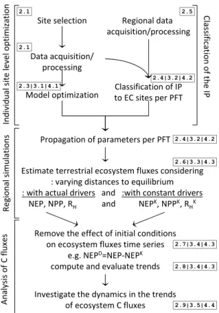
This section describes the bottom-up approach from site level optimization to regional flux estimations and analysis, which is summarized in Fig. 1.
2.1 Eddy flux sites and data
The European network of eddy-covariance measurements sites from the Carboeurope Integrated Project extends from Mediterranean to boreal ecosystems (http://www. carboeurope.org) and has been supporting broad research on processes of mass and energy transfer at the ecosystem level (Aubinet et al., 2000) throughout different vegetation types (Ciais et al., 2010; Luyssaert et al., 2009). Here, we rely on a selection of 33 sites that includes a significant diver-sity of ecosystems representing a significant range of climate regimes and net ecosystem flux magnitudes (Table 1). These sites were selected based on: (1) their representativeness of the ecosystems present in the Iberian Peninsula, though not necessarily located in this region; (2) a minimum data avail-ability of bi-weekly flux integrals with more than 80% of the half-hourly original data or after gap-filling with high confi-dence (Category A in Reichstein et al., 2005). In situ mea-surements of climate variables and MODIS remotely sensed normalized difference vegetation index (NDVI, Huete et al., 2002) were used to drive site level simulations in the inverse model optimization.
2.2 The CASA model
CASA is a process-based biogeochemical model that esti-mates net ecosystem production (NEP) fluxes as the differ-ence between NPP andRH (Field et al., 1995; Potter et al., 1993). The estimates of NPP follow the radiation use effi-ciency approach of Monteith (1972):
NPP=fAPAR·PAR·ε, (1)
wherefAPAR is the fraction of photosynthetically active ra-diation absorbed by vegetation; PAR is the amount of photo-synthetically active radiation; andεis the light use efficiency, which is calculated by down-regulating maximum light use
Site selection
Data acquisition/ processing
Model optimization
Regional data acquisition/processing
Classification of IP to EC sites per PFT
Propagation of parameters per PFT
Estimate terrestrial ecosystem fluxes considering : varying distances to equilibrium : with actual drivers and :with constant drivers
NEP, NPP, RH and NEPK, NPPK, RHK
Remove the effect of initial conditions on ecosystem fluxes time series
e.g. NEPD=NEP‐NEPK
compute and evaluate trends
Investigate the dynamics in the trends of ecosystem C fluxes
Individual
site
level
optimization
Classification
of
the
IP
Regional
si
mulations
Anal
ysis
of
C
fluxes
2.1
2.1
2.3|3.1|4.1
2.5
2.4|3.2|4.2
2.4|3.2|4.2
2.6|3.3|4.3
2.7|3.4|4.3
2.9|3.5|4.4 2.8|3.4|4.3
Fig. 1. Workflow of the current analysis: from site level observa-tions to regional dynamics of ecosystem C fluxes. The model-data integration followed at site level yields optimized parameter vec-tors used for regional simulations. The propagation of parameter vectors is dependent on the classification results of each IP grid-cell according to site level characteristics, which support the sen-sitivity analysis to the initial conditions. Ultimately, the evalua-tion of trends in ecosystem fluxes quasi-independently from initial conditions allows the decomposition of modeled ecosystem fluxes into component fluxes and investigating the underlying dynamics of NEP trends. The numbers in gray boxes indicate the sections of the manuscript focusing on the different aspects of each step: materials and methods (2.x); results (3.x); and discussion (4.x).
efficiency (ε∗
) via the effect of temperature and water avail-ability stress factors (TεandWε, respectively):
ε=ε∗·Tε·Wε. (2)
N.
Carv
alhais
et
al.:
Upscalin
g
ecosystem
C
flux
es
for
the
Iberian
Peninsula
Table 1. Identification of the different sites included in the parameter optimization. The sites are divided by plant functional type (PFT) and the percentage of each site per PFT
and in the IP is shown; as well as the percentage of each PFT in the Iberian Peninsula (PFT in IP). The mean annual temperature (MAT), total annual precipitation (TAP), incoming solar radiation (Rg), climate classification (KG, according to Kottek et al., 2006) and net ecosystem production (NEP) are for the time period (Period). The model efficiency (MEF) is reported as well as the total number of data points per site (total N) and the data points used in the optimization (Filtered N). The different PFTs considered are evergreen broadleaf forests (EBF), deciduous broadleaf forests (DBF), mixed forests (MF), evergreen needleleaf forests (ENF), savannah type ecosystems (SAV), grasslands (GRA), shrublands (SHR) and croplands (CRO). In the climate classification the first letters stand for: C – warm temperate climates, and D – snow climates; the second letters – s, f, or w – stand for the precipitation regimes: dry summer, dry winter or fully humid, respectively; and the third letter classify the temperature: a, b or c, stand for hot summer, warm summer or cool summer and cold winter.
PFT Site Site % in IP MAT TAP Rg KG NEP MEF Filtered N Period Publication (% in IP) (code) (% in PFT) (◦C) (mm yr−1) (W m−2) (class) (gC m−2yr−1) (total N)
EBF, 6.5
FR-Pue 4.06 (62.48) 13.66 941.66 168.27 Csa 221.23 0.7 142 (161) (2000, 2006) Rambal et al. (2003) PT-Esp 2.44 (37.52) 16.95 472.81 209.86 Csa 604.5 0.25 74 (115) (2002, 2006)
DBF, 1.72
DK-Sor 0.00 (0.19) 8.51 1029.9 107.63 Cfb 56.63 0.96 128 (161) (2000, 2006)
FR-Fon 0.03 (1.84) 12.22 668.76 139.22 Cfb 726.5 0.81 39 (46) (2005, 2006) Delpierre et al. (2009) FR-Hes 1.08 (62.82) 10.47 962.86 136.01 Cfb 471.04 0.94 146 (2192) (2000, 2006) Granier et al. (2000) IT-Col 0.41 (23.63) 6.78 914.83 156.4 Cfb 621.56 0.99 25 (92) (2003, 2006) Valentini et al. (1996) IT-Non 0.05 (2.89) 14.41 1205.27 167.49 Cfa 527.48 0.82 47 (69) (2001, 2003) Reichstein et al. (2005) IT-PT1 0.02 (1.41) 15.17 752.31 168.03 Csa 708.49 0.9 57 (69) (2002, 2004) Migliavacca et al. (2009) IT-Ro1 0.12 (7.22) 15.03 875.65 159.51 Csa 159.98 0.8 123 (161) (2000, 2006) Reichstein et al. (2003)
MF, 3.25
BE-Bra 0.70 (21.49) 12.45 733.47 126.76 Cfb 218.04 0.88 42 (69) (2004, 2006)
BE-Vie 2.33 (71.66) 7.53 836.88 99.16 Cfb 420.66 0.91 106 (161) (2000, 2006) Aubinet et al. (2001) DE-Meh 0.22 (6.86) 8.35 511.98 116.93 Cfb −25.08 0.9 75 (92) (2003, 2006)
ENF, 6.88
DE-Tha 0.85 (12.40) 8.6 818.21 120.4 Cfb 522.23 0.76 145 (161) (2000, 2006) Gr¨unwald and Bernhofer (2007) ES-ES1 1.29 (18.69) 17.33 623.73 183.48 Csa 434.3 0.36 132 (161) (2000, 2006) Reichstein et al. (2005) FI-Hyy 0.00 (0.06) 5.63 499.34 106.81 Dwc 257.89 0.94 124 (161) (2000, 2006) Suni et al. (2003) FR-LBr 1.67 (24.33) 14.06 825.17 161.57 Cfb 271.17 0.72 60 (92) (2003, 2006) Ogee et al. (2003) IL-Yat 1.07 (15.49) 16.61 492.58 206.47 Cfa 315.32 0.84 24 (46) (2002, 2003) Grunzweig et al. (2003) IT-Ren 0.63 (9.15) 5.3 1641.62 168.81 Dfc 719.91 0.53 70 (115) (2000, 2004) Montagnani et al. (2009) IT-SRo 1.37 (19.89) 14.59 856.25 152.17 Csa 427.58 0.74 85 (115) (2002, 2006) Chiesi et al. (2005)
SAV, 3.74
ES-LMa 2.52 (67.33) 16.85 768.38 201.75 Csa 91.21 0.8 58 (69) (2004, 2006)
PT-Mi1 1.22 (32.67) 17.43 334.86 225.89 Csa 121.09 0.54 44 (69) (2003, 2005) Pereira et al. (2007)
GRA, 24.81
AT-Neu 0.68 (2.74) 7.85 1379.63 145.87 Dwb −6.9 0.59 70 (92) (2002, 2005) Wohlfahrt et al. (2008) ES-VDA 1.07 (4.30) 8.3 1165.84 200.76 Cwc 130.4 0.5 36 (69) (2004, 2006) Gilmanov et al. (2007) FR-Lq1 4.31 (17.39) 7.73 947.01 136.82 Cfb 189.83 0.74 66 (69) (2004, 2006) Gilmanov et al. (2007) HU-Bug 3.71 (14.94) 8.86 545.73 122.25 Cfb 65.12 0.87 68 (115) (2002, 2006)
IT-Amp 5.98 (24.09) 9.34 1007.67 144.19 Csb 106.36 0.63 69 (115) (2002, 2006) Gilmanov et al. (2007) IT-MBo 0.08 (0.33) 4.86 828.57 154.55 Dwc 104.82 0.79 89 (92) (2003, 2006) Marcolla and Cescatti (2005) PT-Mi2 8.98 (36.20) 14.49 545.85 208.14 Csa 38.21 0.75 50 (69) (2004, 2006)
SHR, 16.76 IT-Noe 16.76 (100.00) 17.6 502.46 216.82 Csa 145.21 0.9 45 (72) (2004, 2006)
CRO, 36.35
BE-Lon 3.66 (10.06) 11.12 731.91 126.15 Cfb 623.04 0.44 54 (69) (2004, 2006) Moureaux et al. (2006) ES-ES2 16.79 (46.20) 18.68 702.32 198.76 Cwa 806.99 0.83 51 (69) (2004, 2006)
FR-Gri 5.18 (14.24) 11.18 500.71 132.77 Cfb 240.39 0.32 46 (46) (2005, 2006) Hibbard et al. (2005) IT-BCi 10.72 (29.50) 16.91 1236.13 181.01 Csa 564.19 0.68 49 (69) (2004, 2006) Reichstein et al. (2003)
7,
3707–
3729
,
2010
www
.biogeoscienc
For site level and regional simulations we estimated
fAPAR as the mean of the two linear scaling methods with the simple ratio and the NDVI, individually per plant func-tional type (PFT), according to Los et al. (2000). We com-puted leaf area index (LAI) as varying exponentially with
fAPAR, or linearly for clustered PFTs (e.g. coniferous trees and shrubs) or as a combination of the previous two for clus-tered and evenly distributed vegetation types, following Sell-ers et al. (1996). The carbon assimilated by vegetation is par-titioned between the different vegetation pools according to the dynamic allocation scheme of Friedlingstein et al. (1999) which adjusts the investments in leaves, stems and roots to-wards the most limiting resource (water, light and mineral nitrogen). Carbon is then transferred from living vegetation pools to soil pools through leaf litter fall, root and wood mor-tality (Potter et al., 1993; Randerson et al., 1996). The cy-cling of carbon between the different soil C pools follows a simplified version of the CENTURY model (Parton et al., 1987).RHis estimated as the integral of decomposition from the different soil C pools:
RH= P X
i=1
Ci·ki·Ws·Ts·(1−Mε), (3)
where each pool i is characterized by a different turnover rateki that is regulated by the effect of temperature (Ts) and water availability conditions (Ws) (Potter et al., 1993). The effect of temperature in decomposition (Ts) follows an ex-ponentialQ10-type response; while the effect of soil water conditions (Ws) is estimated as a non-linear function of the ratio between water availability (soil moisture plus precipita-tion) over the potential evapo-transpiration, following a lin-ear positive response from 0 to 1, with a maximum set for values between 1 and 2, and then decreasing gradually as ex-cess conditions of water supply increase (Potter et al., 1993). The carbon content of each pool (Ci) results from the inte-grated transfers between the different pools, which is further regulated by the carbon assimilation efficiency of microbes (Mε). CASA assumes nine soil carbon pools (P =9) that circulate carbon inputs from vegetation debris and have dif-ferent turnover rates, ranging from monthly (metabolic lit-ter pools) to centennial (old pools) scales. According to the model structure, temperature (Ts) and water availability (Ws) controls on the instantaneous turnover rates equally affect all soil C pools. Higher inertia is seen in the slower turnover soil carbon pools, which take longer to respond to changes in cli-mate conditions and changes in vegetation states – and vice versa. Hence, these pools take longer to reflect a perturbation as well as to recover from it. In general, the robustness of the CASA model has been corroborated by its wide application in studies that range from ecosystem to global scales (e.g., Carvalhais et al., 2008; Randerson et al., 2002) and that fo-cus on different ecological and biogeochemical issues (e.g., Potter et al., 2001; van der Werf et al., 2003).
2.3 Inverse model parameter optimization
in parameter estimation for different sites with different his-torical backgrounds (Carvalhais et al., 2008). The parameter optimization method consisted on the minimization of the sum of residual squares between eddy-covariance measure-ments and model estimates of biweekly NEP fluxes using the Levenberg-Marquardt algorithm (Draper and Smith, 1981). 2.4 Upscaling of model parameters
The upscaling of model parameters aims at attributing pa-rameter vectors optimized at site level, on a per-pixel basis, to the whole Iberian Peninsula. The conceptual idea here is that, within an ecosystem type or PFT, each pixel p in the map would be treated according to its similarity with eddy covariance sitej, and parameterized accordingly. The as-signment of a parameter vector to a given pixel p is supported by a nearest neighborhood classification of the climatic and phenological conditions: to a given pixel p, the parameter vector S corresponding to site j (Sj) is applied when the climate and phenological characteristics of p are closer to j’s than to any other site’s from the same PFT. So,Sp=Sj when d∗
p,j=argminj=1,...,N dp,j
finds the minimum dis-tances between climate and phenological characteristics be-tween a pixel p and an eddy covariance sitej calculated as dp,j=1−NS Vp,Vj. Here, VpandVj are vectors con-taining the normalized biweekly time series of mean air tem-perature, precipitation and solar radiation for the period 1960 to 1990; and mean NDVI between 1982 and 2005. NS is the Nash-Sutcliffe coefficient:
NS Vp,Vj=1−
PN
i=1 Vp,i−Vj,i2 PN
i=1 Vp,i−Vp
2 , (4)
which quantifies the relative association between two vec-tors relative to the association between the reference vector and its mean (the nominal situation) (Janssen and Heuberger, 1995; Nash and Sutcliffe, 1970), whereN is the length of the vectorsVpandVp(N=96) andithe column index of these vectors. In addition to providing a measure of associa-tion, the NS also measures the agreement between two vec-tors (proximity to the 1:1 line). Consequently, the climatic-phenological distance measure (from here on identified as CPd) reflects both the proximity in the magnitude and sea-sonality of climate and phenology drivers between site level observations and the regional datasets for the IP. The results associate one site of each PFT per pixel which means that if a given PFT is present in that pixel the respective parameter vector corresponds to the site where the climate and pheno-logical characteristics are closer to the pixel’s.
2.5 Data for spatial runs
CASA requires drivers related to climate (temperature, pre-cipitation and solar radiation) as well as to biophysical prop-erties of vegetation (NDVI orfAPAR and LAI). Due to the diagnostic nature of CASA, the temporal extent of the model
runs for the Iberian Peninsula was bounded by the longest re-motely sensed NDVI record available: the Global Inventory Modelling and Mapping Studies (GIMMS) NDVI (Tucker et al., 2005). The option of using the biweekly MODIS NDVI products (2 by 2 window of 250 m×250 m pixels) for site level evaluation of the model and the GIMMS NDVI datasets (8 km×8 km pixels) for the regional runs was based on two assumptions: (1) the eddy-covariance footprint de-pends on the local conditions (G¨ockede et al., 2008) and height of the tower (Barcza et al., 2009) but generally is not larger than 1 km2, making the 8 km by 8 km areas too large for representation of the eddy-covariance data; and (2) the MODIS and GIMMS NDVI products are comparable (Tucker et al., 2005). Monthly climate datasets – air temper-ature, precipitation and solar radiation – at 10′spatial
resolu-tion since 1901 until 2000 are available from the Climate Re-search Unit of the University of East Anglia (Mitchell et al., 2004). The climate datasets were extended until 2006 us-ing pixel level empirical relationships with coarser climate datasets. For temperature and solar radiation we made use of 0.25 degrees datasets from the Global Land Data Assimila-tion System (Rodell et al., 2004). PrecipitaAssimila-tion was extended using 0.5 degrees datasets from the University of Delaware (Matsuura and Willmott, 2007). Every dataset was spatially interpolated to the GIMMS NDVI 8 km by 8 km grid follow-ing a weighted average considerfollow-ing a non-linear distance to the four neighboring pixels Zhao et al. (2005). We used lin-ear interpolation to downscale from monthly to biweekly pe-riods. The soil properties – texture fractions and soil depth – were obtained from the Soil Map of the European Communi-ties (The Commission of the European CommuniCommuni-ties Direc-torate General for Agriculture, Coordination of Agricultural Research, 1985). The proportion of each PFT within every 8 km by 8 km pixel is defined by the CORINE land cover map (Bossard et al., 2000). The fraction of forest PFTs is defined by the tree cover value of the MODIS vegetation continu-ous fields at 1 km (Hansen et al., 2003) bounded by the class intervals defined in each CORINE class.
2.6 Regional model runs for a range of initial conditions
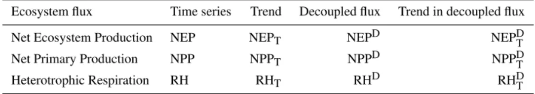
Table 2.Acronyms used to identify the different ecosystem flux components and temporal signals.
Ecosystem flux Time series Trend Decoupled flux Trend in decoupled flux
Net Ecosystem Production NEP NEPT NEPD NEPDT
Net Primary Production NPP NPPT NPPD NPPDT
Heterotrophic Respiration RH RHT RHD RHDT
NEPp=
n X
PFT=1
fPFTp·NEPp,PFT. (5)
for each PFT the model is always spun up with a mean yearly dataset until steady state after which a range of non-equilibrium conditions is forced on the more recalcitrant and microbial soil carbon pools. The prescription of different dis-tances to equilibrium is obtained by multiplying these pools by the scalarηafter the spin-up and then running the model forward. We create a range of initial conditions, from signif-icant sinks (η≪1) to sources (η≫1) by changing theη val-ues between 0.01 and 2 (in 0.1 increments). The ensemble of runs obtained allows evaluating the impacts of different distances to equilibrium in the inter-annual variability and temporal trends in net ecosystem fluxes.
2.7 Decoupling the drivers effects on ecosystem fluxes from the initial conditions
It is recognized that the steady state estimates of the soil car-bon pools are a function of the model parameterization and environmental drivers prescribed for the spin-up (Andr´en and K¨atterer, 1997). Hence, for the same model parameteriza-tion and drivers, any prescribed distance of the soil C pools to equilibrium (η) yields a dynamic recovery response to-wards equilibrium with the simulation drivers. The recovery from a prescribedηcan yield conditions different from the steady state as a response to the simulation’s climate and/or phenology time series. It is essential to distinguish or isolate the effects of the drivers from the recovery dynamics on the ecosystem fluxes. Here, we opted for removing the recov-ery dynamics by performing parallel model runs with con-stant drivers. In these runs the climate and phenology drivers were identical to the spin-up runs datasets: the mean year of the complete 25 year time series. Further, we prescribed the exact same parameterization andηscalars used in the regu-lar forward model runs. To obtain a climate-phenology, not recovery, driven NEP time series (NEPD, Table 2) we sub-tracted the fluxes estimated with the constant drivers (NEPK, Table 2) from the NEP time series:
NEPD=NEP−NEPK. (6)
With this procedure we can remove the variance and tra-jectories of NEP resulting from the soil C pools recovery and investigate the responses of fluxes to the climate and pheno-logical drivers.
2.8 Sensitivity analysis of net ecosystem fluxes to equilibrium assumptions
The sensitivity of the regional decadal fluxes to the initial conditions is assessed by evaluating the changes in inter-annual variability (IAV) and the trends in ecosystem fluxes computed assuming different distances to equilibrium. The reference scenario is always the time series of ecosystem fluxes estimated in equilibrium (η=1, for which NEP is
de-fined as NEPeq). Inter-annual variability is dede-fined as the variance of the annual ecosystem flux integrals over all the years in the analyzed period: 1982 to 2006. The seasonal cycle is removed from the time series for the estimation of temporal trends on the ecosystem fluxes. The seasonal cycle is estimated on a pixel-by-pixel basis using a local variant of Singular System Analysis, as originally introduced by Yiou et al. (2000), as described by Mahecha et al. (2010). This method allows for detection of a highly phase and amplitude modulated seasonal cycle. Based on the deseasonalized time series, the magnitude of the trends is calculated by the Sen slope (Sen, 1968), which is considered a robust estimator of the magnitude of a monotonic trend (Yue et al., 2002). The significance of these trends in the ecosystem fluxes time series is evaluated through the Mann-Kendall test (Kendall and Griffin, 1975; Mann, 1945). The Mann-Kendall test is a non-parametric rank based method that has been widely used to detect the presence of monotonic trends in environmen-tal variables (e.g., Burn et al., 2004; Hamed and Rao, 1998; Kahya and Kalayci, 2004), given its robustness to outliers and because no assumption on data distribution are required. 2.9 Decomposition of ecosystem fluxes
Further, the decomposition of NPP and RH trends into their main drivers may clarify the mechanisms behind sig-nificant trends in both fluxes. The drivers for modeled NPP are remotely sensed NDVI and climate variables, although ultimately their influences are expressed in terms offAPAR and temperature and water availability stress factors trends: TεandWε, respectively. Although the relationships between observed variables and the NPP scalars are non-linear, the scalars themselves all share the same dimensional character-istics – represent fractional properties ranging between 0 and 1 – and yield identical effects on NPP: a 0.1 increase in any of the temperature or water scalars or infAPAR equally yield a 10% increase in NPP (considering the same maximum light use efficiency and solar radiation conditions). In this regard, the isolation of the climatic effects from thefAPAR time se-ries is not mechanistically feasible. Hence, the partitioning of NPP drivers is understood as between the changes in phe-nology (fAPAR, which also integrate effects of climate in the canopy’s structure) and the effects of climate in the instanta-neous light use efficiency (ε).
ForRH, the changes in climate drivers may produce trends in the temperature (Ts) and water (Ws) stress scalars butRH is also influenced by substrate availability. The vegetation pools are the main sources of carbon for RH through the transfer of live biomass to detritus via litter fall, wood and root mortality. The carbon transferred to the soil litter pools then cycles through different soil pools mediated by micro-bial decomposition releasing C throughRH. The changes in substrate can be due to changes in inputs from the vegeta-tion pools or due to changes in rates of consumpvegeta-tion of the substrate. The latter produces a negative feedback onRH in response to environmental conditions: favorable conditions forRHincrease decomposition reducing substrate availabil-ity, and vice versa. The connection between these factors hampers distinguishing between trends in soil C availabil-ity and environmental conditions. Hence we choose to focus on the carbon available for decomposition from the vegeta-tion, which equals the sum of the vegetation pools magnitude weighted by their respective turnover rates. This approach is consistent with the model formulation where the changes in the vegetation pools are directly proportional to the changes in inputs to the soil. Here, the carbon transfers to the soil pools are driven by constant turnover rates for each vegeta-tion pool. The calculavegeta-tions of trends for the carbon pools were estimated relative to the pools’ mean; hence the result is a relative trend, in fractional units, consistent with the units of the environmental scalars.
0 0
NPP T
RH
T
negative NEP trends positive NEP trends RH
T >0
NPP T
<0
NPP T
>0
RH T
<0 NPP
T
<0 & RH T
<0
NPP T
<RH T
RH T
<NPP T NPP
T
<0 & RH T
<0 NPP
T
>0 & RH T
>0
RH T
>NPP T
NPP T
>RH T NPP
T
>0 & RH T
>0
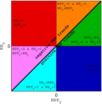
Fig. 2. Abacus of NEPTdecomposition into NPP andRHtrends:
NPPTand RHT, respectively.
3 Results
3.1 Model optimization at site level
Throughout eddy covariance sites the parameter optimiza-tion yields statistically significant correlaoptimiza-tions between ob-servations and model simulations (α <0.0001). The model efficiency (MEF) at site level reflects an overall good agree-ment between simulations and observations (MEF closer to 1, Table 1) and the median of all site level MEF results is 0.79. Overall, the MEF of DBF, MF and SHR is significantly higher than the MEF of the other PFTs (1-way ANOVA,α < 0.0005). Although the mean model performance is higher in temperate fully humid climates, the difference is not sta-tistically significant from the other climatic regimes (1-way ANOVA,α >0.25).
Table 3. Results of the site level parameter optimization organized by plant functional type (PFT): evergreen broadleaf forests (EBF), deciduous broadleaf forests (DBF), mixed forests (MF), evergreen needleleaf forests (ENF), savannah type ecosystems (SAV), grasslands (GRA), shrublands (SHR) and croplands (CRO). The optimized parameters are: maximum light use efficiency (ε∗, [gC MJ−1APAR]), optimum temperature for photosynthesis (Topt, [◦C]), the sensitivity of light use efficiency to water stress (Bwε, [unitless]) and the effect of
temperature (Q10, [unitless]) and water availability (Aws, [unitless]) on heterotrophic respiration (for a detailed description see Carvalhais
et al., 2008). Values in parenthesis report the standard deviation around the mean parameters calculated from the optimized parameters and standard error for all the sites of each PFT.
PFT ε∗ T
opt Bwε Q10 Aws
EBF 0.45 (0.09) 13.55 (6.66) 0.72 (0.27) 2.36 (1.33) 0.63 (0.43) DBF 0.85 (0.21) 17.88 (3.32) 0.66 (0.28) 1.38 (0.68) 0.86 (0.44) MF 0.68 (0.16) 15.18 (4.75) 0.54 (0.15) 1.52 (0.40) 1.19 (0.42) ENF 0.70 (0.18) 14.98 (3.46) 0.64 (0.19) 1.91 (0.85) 0.84 (0.33) SAV 0.30 (0.08) 15.13 (8.19) 0.57 (0.27) 1.13 (0.92) 0.60 (0.26) GRA 1.19 (0.86) 6.44 (2.63) 0.72 (0.26) 1.46 (0.54) 1.12 (0.77) SHR 2.14 (0.24) 7.40 (0.93) 0.87 (0.09) 2.88 (0.72) 0.30 (0.07) CRO 1.04 (0.30) 20.77 (7.52) 0.58 (0.22) 1.97 (1.31) 1.30 (0.97)
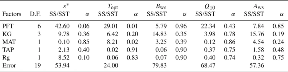
Table 4.N– way ANOVA results (%) for each optimized parameter for each factor: PFT – plant functional type; climate classification (KG) (according to Kottek et al., 2006); MAT – mean annual temperature; TAP – total annual precipitation; and Rg – incoming solar radiation. The results presented: SS – sum of squares; SST – total sum of squares;α– significance test result for each factor. The KG snow climate classes (D) were integrated within the same group and the warm temperate classes aggregated according to precipitation regimes (second letter), to avoid classes with only one site. We removed SHR from the test, since it only has one site, and grouped the climate classification in one class including all snow climates and the other classes per annual temperature and precipitation regime, to avoid having classes with one site. D.F. stands for degrees of freedom.
ε∗ T
opt Bwε Q10 Aws
Factors D.F. SS/SST α SS/SST α SS/SST α SS/SST α SS/SST α
PFT 6 42.60 0.06 29.01 0.01 5.79 0.96 22.34 0.43 7.84 0.85
KG 3 9.78 0.36 6.42 0.20 14.83 0.35 3.98 0.78 15.76 0.19
MAT 1 0.10 0.85 8.21 0.02 3.25 0.39 0.12 0.86 4.54 0.24
TAP 1 2.13 0.40 0.02 0.91 0.06 0.90 0.37 0.75 1.58 0.48
Rg 1 8.52 0.10 0.06 0.83 0.07 0.90 0.40 0.74 0.32 0.75
Error 19 53.94 24.00 79.83 68.47 57.36
Overall, the optimization results at site level show signif-icant confidence in the CASA model performance for sites representing the PFTs of the IP domain, where the average MEF weighted by PFT fraction is 0.73.
3.2 Upscaling parameter vectors for the IP
The map of the distances in climatological and phenological space (CPd) between individual pixels and the eddy covari-ance sites shows that in general the IP domain is well rep-resented by the group of eddy covariance sites used in this analysis (Fig. 3).
For the entire Iberia, 94% of the pixels show a weighted CPd between pixel’s and site characteristics below 1 – the nominal situation – meaning that, on average, the associa-tion between the chosen site for a given pixel is better than just considering the average of the target pixel (Schaefli and Gupta, 2007). The median distance (CPd) is 0.56, indicating
a significant association between the drivers from the eddy covariance sites and from the regionalized datasets.
The NW region shows systematic higher CPdto the eddy covariance sites characteristics (Fig. 4) and emphasizes the low local representativeness for all PFTs in the region. Mixed forest, crops and grasslands each contribute about 20% of the total land cover in this region; hence, substantial improve-ments in the region’s representativeness would be achieved by including in our analysis eddy covariance sites monitoring such PFTs with more similar phenology and climate charac-teristics.
−8 −6 −4 −2 0 2 36
37 38 39 40 41 42 43
0 0.2 0.4 0.6 0.8 1 1.2 1.4 1.6 1.8 2
0 0.035
Frequency
Fig. 3. Spatial patterns of the representativeness of the eddy covari-ance sites for pixels of the Iberian Peninsula. The distcovari-ance measure (CPd) of each pixel is computed as the average CPdweighted by
the fraction of all the sites used for its parameterization. The right side histogram shows the frequency of the observed CPdfor all the
pixels in Iberia (Eq. 4).
3.3 Changes in Inter-Annual Variability (IAV)
Inter-annual variability in NEP is higher for the farthest non-equilibrium initial conditions (observed at very low and high ηprescriptions, Figs. 5, 4a). The modeling results show re-gional increases of 47% and 174% in IAV for the lowest and highest η, respectively, considering the average fluxes for the whole domain of the IP (Fig. 5b, inset plot line a). The changes in IAV show significant increases in spatial variabil-ity with distance to equilibrium (Fig. 5a). These are driven by the changes in the IAV ofRH, which are strongly dominated by the recovery of the carbon pools (Fig. 6a).
The removal of C pools recovery from the prescribedη (Eq. 6) significantly reduces the changes in IAV caused by distance to equilibrium (Fig. 5b). The highest changes are still observed for extremeηvalues although these are modest compared to the previous results, with regional changes of
−3% and 7% forηof 0.01 and 2, respectively. Nevertheless, the spatial variability of IAV changes still increases with dis-tance to equilibrium (Fig. 5b). The changes that still exist between the ratio of IAV of NEPDand the IAV of NEPeqfor differentηvalues are driven by changes in the IAV ofRDH, which respond proportionally to the varying magnitude of soil carbon pools for differentη(Fig. 6b). A highηincreases the carbon pools which increase the magnitude of the IAV in RHDand its role in the IAV of NEPD. Conversely, lowηvalues reduce the role of RDHin the IAV of NEPD, and increase the role of the IAV in NPPDin the IAV of NEPD. Consequently, the effects on the IAV of NEPDare stronger for larger carbon sources (η≫1) and sinks (η≪1) (Fig. 5b), but these do not follow theRDHpatterns.
Overall, the results show that regionally both approaches reveal significant differences between each other (Fig. 5b, inset plot), which originate exclusively from the recovery of carbon pools from the prescribed initial disequilibrium conditions. The similarity between the IAV of the different
Table 5.Percentage of positive, negative and non-significant trends in NEPeqand NEPDfor the Iberian Peninsula.
NEPeq
Trend Negative Not significant Positive Total
NEP
D NegativeNot significant 8.563.25 54.410.45 0.006.44 64.099.01
Positive 0.00 0.29 26.62 26.90
Total 11.81 55.14 33.05
NEPD suggests quasi-independence from the initial condi-tions. The slight changes observed in the IAV of NEPDstem not from the recovery from the initial conditions but from the carbon pools sizes.
3.4 Temporal trends for the IP
The evaluation of trends in NEP shows that the spatial dis-tribution of its magnitudes (Sen slope) is strongly influenced by the prescribed initial distance to equilibrium (Fig. 7a), as expected. On the other hand, the distribution of NEPDtrend magnitudes appears to beηinvariant (Fig. 7b) and suggests independence from the pools’ initial conditions. The spatial distribution of the significant trends in NEP in equilibrium (NEPeq, Fig. 7c) differs only slightly from the map of mean NEPD trends (Fig. 7d). The Mann-Kendall test yields non significant trends in NEP for 55% of the IP, while about 64% of the IP shows non significant trends for NEPD. The area difference of negative trends in the IP between NEPeq and NEPDis about +3%, while the difference in the area of posi-tive trends is about +6% (Table 5). Overall, both approaches agree almost 90% of the time on the type of trend (nega-tive, positive or non significant) and the spatial NS between NEPeq and NEPD is 0.99. Consequently, these differences are considered minor. These results show significant trends in NEPDdriven exclusively by climate and phenology. A di-rect implication of these results is the ability of the approach to detect climate and phenology induced trends that are inde-pendent of the initial carbon pools.
3.5 Determinants of temporal trends in the IP
−8 −6 −4 −2 0 2 36 38 40 42 0.2 0.4 0.6 0.8 1
FR−Pue
PT−Esp
EBF−8 −6 −4 −2 0 2 36
38 40 42 0 1 2
−8 −6 −4 −2 0 2
36 38 40 42 0.2 0.4 0.6 0.8 1
DE−Hai
DK−Sor
FR−Fon
FR−Hes
IT−Col
IT−Non
IT−PT1
IT−Ro1
DBF
−8 −6 −4 −2 0 2 36
38 40 42 0 1 2
−8 −6 −4 −2 0 2
36 38 40 42 0.2 0.4 0.6 0.8 1
BE−Bra
BE−Vie
DE−Meh
MF
−8 −6 −4 −2 0 2 36
38 40 42 0 1 2
−8 −6 −4 −2 0 2
36 38 40 42 0.2 0.4 0.6 0.8 1
DE−Tha
ES−ES1
FI−Hyy
FR−LBr
IL−Yat
IT−Ren
IT−SRo
ENF
−8 −6 −4 −2 0 2 36
38 40 42 0 1 2
−8 −6 −4 −2 0 2
36 38 40 42 0.2 0.4 0.6 0.8 1
ES−LMa
PT−Mi1
SAV−8 −6 −4 −2 0 2 36
38 40 42 0 1 2
−8 −6 −4 −2 0 2
36 38 40 42 0.2 0.4 0.6 0.8 1
AT−Neu
ES−VDA
FR−Lq1
HU−Bug
IT−Amp
IT−MBo
PT−Mi2
GRA
−8 −6 −4 −2 0 2 36
38 40 42 0 1 2
−8 −6 −4 −2 0 2
36 38 40 42 0.2 0.4 0.6 0.8 1
IT−Noe
SHR−8 −6 −4 −2 0 2 36
38 40 42 0 1 2
−8 −6 −4 −2 0 2
36 38 40 42 0.2 0.4 0.6 0.8 1
BE−Lon
ES−ES2
FR−Gri
IT−BCi
CRO
−8 −6 −4 −2 0 2 36
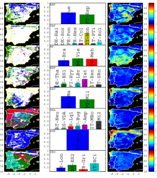
38 40 42 0 1 2
Fig. 4. The classification of the Iberian Peninsula according to the optimized eddy covariance sites per PFT (left column) is based on the selection of the closest site to each pixel. The distance (CPd) maps per PFT show the minimum distance (CPd) from the set of sites to the
IP region (right column). Overall, the spatial classification shows a predominant selection of southern European and Mediterranean sites (middle column). Systematic higher distances (CPd) in the NW IP are observed throughout PFT (right column). White regions in the left
column maps indicate only a residual presence (<5%) of the respective PFT.
of the negative trends in NEPDin the IP); negative or positive trends simultaneously in both fluxes, where the magnitude of the slope of RHDT is higher than the slope of NPPD (cover-ing∼30% and∼17%, respectively). These results are only
slightly different from the trends resulting from the time se-ries of NEPeq(Table 6). Overall, the trends in the IP forRDH and NPPDare predominantly positive.
The NPPDtrends are a result of the trends in stress scalars on light use efficiency driven by temperature and water avail-ability (Tε and Wε, TεT and WεT, respectively) and with
trends infAPAR (fAPART). The trends observed in NPPD (NPPDT) are mainly driven by trends infAPAR (Fig. 10). The spatial partial correlation between the trends infAPAR and NPPDT is significantly higher than between TεT and NPP
D T, 0.79 compared to 0.10, respectively (Table 7). The
magni-tude of theWεtrends was found to be an order of magnitude belowfAPARTandTεT (Fig. 11). However, the spatial
par-tial correlation between WεTand NPPDT is 0.25: significantly higher than the one found forTεT. Overall, these results
sug-gest a significant role offAPAR time series in the productiv-ity trends for the Iberian region.
0.01 0.5 1 1.5 2 1
2 3 4 5 6
var(NEP)/var(NEP
eq
)
η (a)
0.01 0.5 1 1.5 2 1 2 3 4 5 6
var(NEP
D )/var(NEP
eq
)
η (b)
0 0.5 1 1.5 2
0.5 1 1.5 2 2.5 3
η
NEP IAV Changes in IP
a b
Fig. 5. Influence of distance to equilibrium (η) in the inter-annual variability (IAV) of net ecosystem fluxes(a)and in the IAV of the de-trended NEP fluxes (removing the sole recovery from the C pools)(b). Each vertical rectangular box represents the spatial distribution of the IAV ratio indicated in the yy-axis for Iberian Peninsula (all pixels). Rectangular boxes are bounded by 25 and 75 percentile bottom and top, respectively, while the horizontal line inside indicates the sample median; dashed lines limited by horizontal bars indicate the extent of the remaining data, excluding outliers; dot signs (•) indicate statistical outliers. The inset in (b) shows for a spatial average of all the Iberian Peninsula the ratio between the IAV of NEP and the IAV of NEPeq(black line a) and the ratio between the IAV of NEPDand the
IAV of NEPeq(grey line b). The regional differences in IAV for the Iberian Peninsula between both approaches as a function of distance to
equilibrium are significant.
0.01 0.5 1 1.5 2
0 2 4 6 8 10 12 14 16 18
var(R
H
)/var(RH
eq
)
η
(a)
0.01 0.5 1 1.5 2
0 2 4 6 8 10 12 14 16 18
var(R
H
D )/var(RH
eq
)
η
(b)
0 0.5 1 1.5 2
0 1 2 3 4 5 6
η RH
IAV Changes in IP
a b
Fig. 6. Influence of distance to equilibrium (η) in the IAV of heterotrophic respiration (RH) fluxes(a)and in the IAV of the de-trended
RHfluxes (RHD), removing the sole recovery from the C pools)(b). Each vertical rectangular box represents the spatial distribution of the
IAV ratio indicated in the yy-axis for Iberian Peninsula (all pixels). Rectangular boxes are bounded by 25 and 75 percentile bottom and top, respectively, while the horizontal line inside indicates the sample median; dashed lines limited by horizontal bars indicate the extent of the remaining data, excluding outliers; dot signs (•) indicate statistical outliers. The inset in (b) shows for a spatial average of all the Iberian Peninsula the ratio between the IAV ofRHand the IAV of RHeq(black line a) and the ratio between the IAV ofRHDand the IAV of RHeq
Trends of NEP
eq (α<0.05)
−8 −6 −4 −2 0 2
36 37 38 39 40 41 42 43
−10 −5 0 5 10
−10 −5 0 5 10
0 0.01 0.02 0.03
Sen slope of NEP
Frequency
η
0.01 2
Mean trends of NEPD (α<0.05)
−8 −6 −4 −2 0 2 36
37 38 39 40 41 42 43
−10 −5 0 5 10
−10 −5 0 5 10
0 0.01 0.02 0.03
Sen slope of NEPD
Frequency
η
0.01 2
(c) (a)
(d) (b)
Fig. 7. The distribution of the NEP trends (Sen slopes, gC m−2yr−2) is strongly dependent onηvalues(a)while for NEPDits distribution appears invariant withη(b). The spatial pattern of the significant NEP trends for equilibrium conditions(c)only slightly differs from the mean trends for NEPD(d). Per pixel, an NEPDtrend is only considered significant when for allηused in the simulation the significance level is systematically lower than 0.05 and the trend’s signal is consistent (always positive or always negative). The trend is then calculated as the mean of NEPD time series for allηs. Any slope trend is only considered positive or negative when its absolute value is at least 1.5 gC m−2yr−2.
Trends of NEPD
−8 −6 −4 −2 0 2
36 38 40 42
−10 −5 0 5 10
Trends of NPPD
−8 −6 −4 −2 0 2
36 38 40 42
−10 −5 0 5 10
Trends of R H D
−8 −6 −4 −2 0 2
36 38 40 42
−10 −5 0 5 10
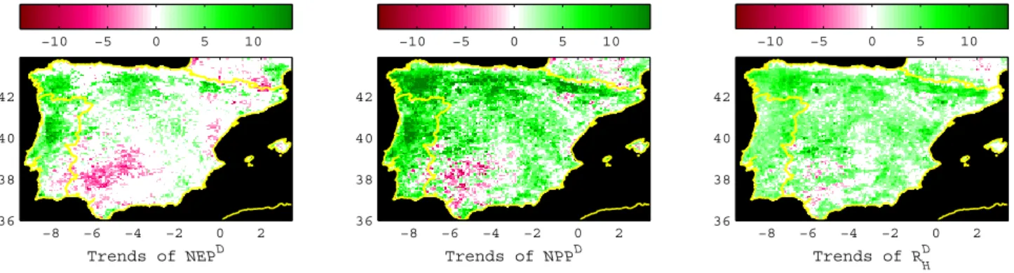
Fig. 8. Mean significant trends in NEPD, NPPDandRDH(gC m−2yr−2). The trends in fluxes in each pixel are considered significant when
Fig. 9. Decomposition of NEPDtrends intoRHDand NPPDtrends (NEPDT, RHDT and NPPDT, respectively – gC m−2yr−2)(a). The spatial
distribution of the underlying NPPDT and RHDT dynamics behind NEPDtrends can be mapped by colour-coding each NEPDTaccording to its position in (a) following the diagram in(c). The colour intensity in(b)is proportional to the magnitude of NEPDT.
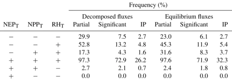
Table 6.Results for the decomposition of NEP trends into NPP andRHtrends for NEPDand NEPeq. The partial frequencies are estimated
dividing the occurrence of NPPTand RHTcombinations by the total occurrence of positive or negative trends (depending on the NEPT
column). Significant frequencies are calculated dividing the occurrence of NPPTand RHTcombinations by the total of significant trends for
the IP region. The fraction of significant trends over the Iberian Region is identified with IP.
Frequency (%)
Decomposed fluxes Equilibrium fluxes NEPT NPPT RHT Partial Significant IP Partial Significant IP
− − − 29.9 7.5 2.7 23.0 6.1 2.7
− − + 52.8 13.2 4.8 45.3 11.9 5.4
− + + 17.3 4.3 1.6 31.6 8.3 3.7
+ + + 97.3 72.9 26.2 97.6 71.9 32.3
+ + − 2.7 2.1 0.7 2.4 1.8 0.8
+ − − 0.0 0.0 0.0 0.0 0.0 0.0
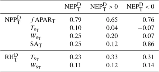
RHDand its drivers’ are not very different between substrate availability (0.25) and temperature (0.23), and are lower for the water stress scalars (0.11). These correlations change sig-nificantly when considering only negative trends in the NEP, where the substrate availability explains 86% of the spatial variability, emphasizing the role of substrate availability in theRHDtrends (Table 7).
4 Discussion
4.1 CASA model optimization
Globally, the site level optimization supports significant confidence in CASA’s performance. In general, the op-timized parameters (Table 3) are within published results (e.g., K¨atterer et al., 1998; Kirschbaum, 1995; Ruimy et al.,
1994) although two different situations are worth mention-ing: (i) the lowToptvalues found for grasslands; and (ii) the high uncertainties in croplands ε∗
andTopt. The low Topt values found for grasses are border line or below the 10◦
C to 25◦
C range for C3 and 30◦
C to 40◦
C for C4 plants, al-though some C3 species are quite active at 5◦
C (Breymeyer et al., 1980). Most of these sites are C3, with the exception of PT-Mi2 which is a C3/C4 mix. Site level records show the occurrence of high gross primary production (95 per-centile) at temperatures below 10◦C. The coherence between
Fig. 10. Decomposition of NPPDtrends (gC m−2yr−2) intoT
ε andfAPAR trends,TεT andfAPART, respectively (fractional units per
square meter per year)(a). The spatial distribution of the underlyingTεT andfAPARTdynamics behind NPP
Dtrends can be mapped by
colour-coding each NPPDT according to its position in (a) following the diagram in(c). The colour intensity in(b)is proportional to the magnitude of NPPDT.
plants grow due to higher moisture availability (e.g. winter or spring). This is consistent with the comparison betweenTopt of grasses and the mean monthly temperatures for the Iberian Peninsula, where the confidence bounds ofToptinclude the monthly temperatures observed during colder months. How-ever, from a model-data integration perspective both model drivers as well as model structure can influence the actual values of parameters. The higher uncertainties in cropland parameters suggest the need to improve/adapt model dynam-ics in agricultural systems, including the prescription of dif-ferent root to shoot ratios according to crop type (e.g., Bon-deau et al., 2007) and explicit harvest events, with above ground biomass removals (e.g., Hicke and Lobell, 2004; Lo-bell et al., 2006), as well as different management regimes considering crop rotation, fertilization, irrigation and tillage practices. These dynamics were not included in the current model implementation. Nevertheless, the good model perfor-mance as indicated by MEF in croplands (Table 1) suggests that the phenology time series acquired from remote sensing captures most of the variability of the NPP. Further, in site level optimizations, the lack of harvest removal of C from the leaf pools that then feeds the soil pools can be approxi-mated by reductions inη. For the purpose of this study, the absence of such dynamics in model simulations is unlikely to change our results.
4.2 Upscaling parameter vectors for the IP
The results reveal systematic lower representativeness in the Northwestern IP region which is generally identified as a high productivity area in regional and global studies (e.g., Jung et al., 2008). Representativeness in this region is low for all PFTs (Fig. 4), which reveals that the under-representation
Table 7. Partial correlations between the trends in NPPD(NPPDT) andRHD(RHDT) and trends in its drivers:fAPAR, temperature (Tε)
and water availability (Wε) effects onε∗(fAPART,TεT andWεT,
respectively) for NPPDT; and substrate availability (SA), tempera-ture (Ts) and soil moisture (Ws) effects on microbial decomposition
(SAT,TsTandWsT, respectively) for RH
D T.
NEPDT NEPDT>0 NEPDT<0 NPPDT fAPART 0.79 0.65 0.76
TεT 0.10 0.04 −0.07
WεT 0.25 0.20 0.07
SAT 0.25 0.12 0.86
RHDT TsT 0.23 0.33 0.31
WsT 0.11 0.12 0.14
is related to the phenological and climate variables used in the classification. Improved representativeness in this region will require more flux measurements from mixed forests, crops or grassland sites with similar bioclimatic character-istics. Further, only one observational site was available rep-resenting shrub lands for the entire IP.
Fig. 11. Decomposition of NPPDtrends (gC m−2yr−2) intoWεandfAPAR trends,WεT andfAPART, respectively (fractional units per
square meter per year)(a). The spatial distribution ofWεT andfAPARTbehind the NPPD trends can be mapped by colour-coding each
NPPDT according to its position in (a) following the diagram in(c). The colour intensity in(b)is proportional to the magnitude of NPPDT.
Fig. 12. Decomposition ofRHDtrends (gC m−2yr−2) intoT
s and substrate availability trends,TsT and SAT, respectively(a). The spatial
distribution ofTsTand SATbehind theR
D
Htrends can be mapped by colour-coding each RHDT according to its position in (a) following the
diagram in(c). The colour intensity in(b)is proportional to the magnitude of RHDT.
support to the conceptual approach taken here to upscale the CASA model parameters. However, there is still a signifi-cant fraction of unexplained variability in the parameters and our bottom-up approach does not address issues related to the variability of parameters within the same PFT or climate regime. Increasing the number of sites and including other factors in the analysis – such as disturbance or management regimes – are two important issues to consider towards more comprehensive upscaling and modeling exercises. In this regard we recognize the importance of prescribing manage-ment (e.g., Bondeau et al., 2007) or disturbance (e.g., van der Werf et al., 2003) regimes, as well as the effects of nutrients dynamics (e.g., Zaehle et al., 2010).
4.3 Dynamics of ecosystem fluxes induced by climate and phenology
The effects of different initial conditions on the IAV and temporal trends in NEP were higher for the highest de-partures from equilibrium, as expected. Since the spin-up routines were performed with an average climate and phenology dataset, the modeled recovery from the initial perturbations (η) is expected to lead to similar ecosystem states (carbon pools). The farthest positive departures from equilibrium (NEP ≫0 since η≪1) create an initial sink
Fig. 13. Decomposition ofRHDtrends (gC m−2yr−2) intoWsand substrate availability (SA) trends,WsTand SAT, respectively (fractional
units per square meter per year)(a). The spatial distribution ofWsT and SATbehind theR
D
Htrends can be mapped by colour-coding each
RHDT according to its position in (a) following the diagram in(c). The colour intensity in(b)is proportional to the magnitude of RHDT.
carbon is accumulated in the soil pools with time, enhancing RH through increases in substrate availability, and therefore decrementing NEP in time. Oppositely, the farthest negative departures from equilibrium (NEP≪0 sinceη≫1) force an initial carbon source by increasing the soil pools. The in-crease in substrate availability boostsRHin the beginning of the simulation which is reduced in time, generating a positive trend in NEP. Consequently, the highest changes in the IAV of NEP are observed when extreme departures from steady state are prescribed.
The extraction of the carbon pools dynamics (NEPK) from the NEP time series allows the exploration of the impact of non steady state conditions in the purely climate and phe-nology driven dynamics of NEP (NEPD). The significant re-duction in IAV changes (Fig. 5) and the distribution of the NEP trends withη(Fig. 7a) emphasize the role of the carbon pools dynamics in the estimation of ecosystem fluxes. These results show that simulated net ecosystem fluxes can strongly diverge depending on initial conditions assumptions. Addi-tionally, the trends in the NEPD time series show a strong insensitivity toηrevealing independence from the initial es-timates of C pools (Fig. 7b). The results exhibit the poten-tial of NEPDto isolate and diagnose climate and phenology driven trends in ecosystem fluxes. By identifying significant and consistent trends in NEPDwe’re able to map regions of robust trends in the Iberian region.
The differences between the spatial distribution of trends in NEPD and NEPeqare minor and reveal that here the cli-mate and phenology driven dynamics are quasi-independent from the initial steady state conditions (Fig. 7c, d). Using a mean yearly dataset of drivers during the period 1982–2006 ensures the adjustment of carbon pools to the mean of the drivers of the run. The adjustments follow first order
dy-namics that are intrinsic to the model structure (CASA’s and many other biogeochemical models). This means that we can isolate the effects of unknown initial conditions by removing NEPK from NEP. The result is the retrieval of a time series of NEPDthat is quasi-independent from the initial conditions of carbon pools. In the current experiments these indepen-dent trends are analogous to the trends in NEPeqbecause the dataset that drives NEPKis equal to the spin-up dataset. Con-sequently, as an alternative to spinning up the models until equilibrium this approach has advantages for exploring the effects of drivers on net ecosystem fluxes independently of the initial conditions of pools.
We should add that ultimately the overall absolute NEP trends are not independent from the initial conditions. Al-though removing carbon pools dynamics from the ecosystem fluxes may allow independence from equilibrium assump-tions, such a procedure does not solve the initial state prob-lem and our ability to quantify temporal trends is still limited. Beside model structure the estimated fluxes depend not only on the model drivers – climate and phenological drivers – but also on the parameters estimated at site level. In this regard, the exhaustive accounting of terrestrial C fluxes implies the explicit integration of disturbances and management regimes that were not simulated – especially agriculture and fire – for the estimation of net biome production (Chapin et al., 2006). In addition, the extension of the current exercise to living pools in non equilibrium conditions can be aided by prospec-tive remotely sensed estimations of above ground biomass. 4.4 Decomposition of ecosystem fluxes
behind the positive and negative trends in NEPD. For most of the Iberian region the positive trends in NEPDare associ-ated with positive trends in NPPD and inRDH, although the slope magnitudes are higher for NPPD. These results are consistent with recent modeling studies (Piao et al., 2009a) and with eddy covariance based studies that advocate the significant role of gross primary production in driving NEP (e.g., Baldocchi, 2008; Reichstein et al., 2007). The positive trends in NPPD are more strongly linked to positive trends infAPAR than to the climate effects on light use efficiency. SincefAPAR estimates are based on the NDVI datasets, the modeled positive NPP trends are mostly driven by phenolog-ical data rather then climate data. ThefAPAR time series are estimated from NDVI (following Los et al., 2000), hence the trend results demonstrate the role of NDVI time series in driving the trends in NPP (cf. Jung et al., 2008).
The close association between climate and vegetation im-plies that the NDVI signal itself contains the effects of cli-mate regimes and patterns in the phenological characteristics of the vegetation (e.g., Myneni et al., 1997). In the CASA model the temperature stress scalars are conceptually associ-ated to adjustments in autotrophic respiration costs while the water stress on canopy productivity can be ascribed to reduc-tions in stomatal conductance (Potter et al., 1993). However, the plants’ response mechanisms to environmental stress can yield impacts on APAR,ε or both. In this regard, current studies have highlighted the limitations of using NDVI or
fAPAR to detect instantaneous light use efficiency changes as a function of water and temperature stress (e.g., Goerner et al., 2009; Grace et al., 2007). It is then implicit in the model structure that the environmental effects onεand on
fAPAR are complimentary for the estimation of NPP and act at different time scales. Hence, here, only the effects of tem-perature and water availability on light used efficiency can be decomposed from the primary productivity signal.
The main mechanism behind positive trends in the net ecosystem fluxes originates from increases in primary pro-duction (mostly driven by fAPAR) that consequently in-crease the vegetation carbon pools and the substrate avail-ability for heterotrophic respiration. Here, the impact of sub-strate availability is in general significantly higher than the effects of temperature or soil moisture on the trends inRDH.
In areas of negative NEPD trends the partial correlation between the spatial patterns of trends in RHD and substrate availability is significantly higher than in areas of positive NEPD trends (Table 7). In these cases (NEPDT <0) the crements in substrate availability are not attributable to in-creases in NPP, since most of the trends infAPAR (89%) as well as in NPPD (83%) are negative. Here, when RHDT>0, the positive trends in substrate availability (75%) are mainly associated to positive trends in the root pools (88%). These positive trends in the root pools are contrary to the trends observed in NPPD. This apparent contrary behaviour results from increases in the carbon allocated to the below ground vegetation pools caused by negative trends in the water stress
scalars ofε∗(88%), increasing water stress. The investment
in the root pools is associated with the increasing trends in water stresses and is consistent with the dynamic allocation scheme by Friedlingstein et al. (1999). Due to the higher turnover rates of the fine root pools – compared to the wood pools – the changes in the allocation strategies increase the availability of carbon for decomposition. These observa-tions highlight that the contribution of climate for long term changes in heterotrophic respiration cannot be dissociated from the availability of material for decomposition (Trum-bore and Czimczik, 2008).
5 Conclusions
Our bottom-up approach allowed us to investigate the in-fluences of the initial conditions in modeling regional net ecosystem fluxes. Overall, the site level optimization results showed significant confidence in model performance. Ac-cording to our approach the set of sites selected is, in general, significantly representative of the climate-phenology condi-tions observed through different PFTs in the Iberian Penin-sula. The resulting spatial patterns highlight the Northwest-ern region as a location of systematic poorer representative-ness ability for the selected climate-phenology descriptors. Consequently, the CASA model reveals itself as a robust di-agnostic approach to estimate NEP fluxes and the methodol-ogy to upscale parameter vectors allows the identification of less represented regions. The presented bottom-up approach emphasizes the relevance of analogous methods for the de-sign of ecosystem monitoring networks.
The influence of the initial conditions on NEP trends and inter-annual variability is significant, as expected. However, we present a method to distinguish between the model in-trinsic dynamics following initialization routines and the flux variability only induced by the driver data. Consequently, we are able to investigate the inter-annual variability and trends in fluxes quasi-independently from the initial conditions. The relevance of such approach emerges from the fact that most of the time the initial conditions of regional or global simu-lations are unknown.