The 2009–2010 step in atmospheric CO<sub>2</sub> inter-hemispheric difference

(1)

BGD

12, 15087–15109, 2015

The 2009–2010 step in atmospheric CO2

inter-hemispheric difference

R. J. Francey and J. S. Frederiksen

Title Page

Abstract Introduction

Conclusions References

Tables Figures

◭ ◮

Back Close

Full Screen / Esc

Printer-friendly Version

Interactive Discussion

Discussion

P

a

per

|

Discussion

P

a

per

|

Discussion

P

a

per

|

Discussion

P

a

per

|

Biogeosciences Discuss., 12, 15087–15109, 2015 www.biogeosciences-discuss.net/12/15087/2015/ doi:10.5194/bgd-12-15087-2015

This discussion paper is/has been under review for the journal Biogeosciences (BG). Please refer to the corresponding final paper in BG if available.

The 2009–2010 step in atmospheric CO

₂

inter-hemispheric di

_ff

erence

R. J. Francey and J. S. Frederiksen

Earth System Assessment, CSIRO Oceans and Atmosphere Flagship, Aspendale, Australia

Received: 6 August 2015 – Accepted: 19 August 2015 – Published: 11 September 2015

Correspondence to: R. J. Francey ([email protected])

(2)

BGD

12, 15087–15109, 2015

Title Page

Tables Figures

◭ ◮

Back Close

Full Screen / Esc

Discussion

P

a

per

|

Discussion

P

a

per

|

Discussion

P

a

per

|

Discussion

P

a

per

|

Abstract

The annual average CO2 difference between baseline data from Mauna Loa and the

Southern Hemisphere increased by ∼0.8 µmol mol−1 (0.8 ppm) between 2009 and

2010, a step unprecedented in over 50 years of reliable data. We find no evidence for coinciding, sufficiently large and rapid, source/sink changes. A statistical anomaly

5

is unlikely due to the highly systematic nature of the variation in observations. An expla-nation for the step, and the subsequent 5 year stability in this north–south difference, involves inter-hemispheric atmospheric exchange variation. The selected data describ-ing this episode provide a critical test for studies that employ atmospheric transport models that interpret global carbon budgets and inform management of anthropogenic

10

emissions.

1 Introduction

The 2009–2010 increase in annual mean CO₂ difference between hemispheres,

∆CN−S, was noted by Francey et al. (2013) using data from Mauna Loa (mlo, 20◦N,

156◦W, altitude 3.4 km) and Cape Grim (cgo, 41◦S, 145◦E, 0.2 km) or South Pole (spo,

15

90◦S, 2.8 km). They reported failure of a global carbon cycle inversion model to reach consistency between the∆C measurements and reported source–sink changes.

Their data, extended here, are based on Commonwealth Scientific and Industrial Re-search Organisation (CSIRO, Australia) flask sampling. Comparisons in Fig. 1a high-light the largely consistent measurements from the 1990s using data from the

Na-20

tional Oceanic and Atmospheric Administration (NOAA, Dlugokencky et al., 2014) and Scripps Institution of Oceanography (SIO, Keeling et al., 2009) networks. A compari-son is also made with a linear regression through the SIO 5-decade_∆C_mlo-sporecord. The historic SIO record shows an increase attributed to the increase in Fossil Fuel (FF) emissions (Le Quéré et al., 2014), which occur predominantly in the Northern

Hemi-25

(3)

BGD

12, 15087–15109, 2015

Title Page

Tables Figures

◭ ◮

Back Close

Full Screen / Esc

Discussion

P

a

per

|

Discussion

P

a

per

|

Discussion

P

a

per

|

Discussion

P

a

per

|

scaled to run parallel to the∆C slope in order to emphasize the unusual nature of the 2009–2010∆C step. From this perspective the 0.8 ppm step, if the result of an anoma-lous flux, would equate to a 1.6 Pg C yr−1 (NH) source. Also obvious in Fig. 1a is the unusual post-2009∆C stability compared to the earlier record.

The dC/dtin Fig. 1b show inter-annual variability on 3 to 5 year El Niño–Southern

5

Oscillation (ENSO) timeframes, forced primarily by climate variability on the equatorial land biosphere (Rayner et al., 2008). This variability is largely suppressed in∆C when resulting CO2is mixed into both hemispheres. Methods to obtain ∆C and dC/dt from

monthly data are descibed in Appendix A.

The hemispheric representativeness of extra-tropical baseline data from the selected

10

monitoring sites is supported by a study of aircraft vertical profiles at 12 global sites, identifying mlo and cgo as being the least affected by surface CO2exchanges in their

respective hemispheres (Stephens et al., 2007). While the spo data closely track cgo data and other mid-to-high southern latitude (SH) sites in the CSIRO network (Francey et al., 2013), the situation is less clear for mlo because of NH heteorogeneity and

15

downwind proximity to Asia. A possible contributing factor at mlo may result from ge-ographical susceptibility to rapidly increasing SE Asian pollution, “rapidly transported to the deep tropics” (Ashford et al., 2015). However in the Supplement Fig. S1 we demonstrate similarity in year-to-year changes in ∆C using both Pacific and Atlantic extra-tropical NH sites from the NOAA network. The similarity is particularly

signifi-20

cant in sign and magnitude for the two largest observed changes in 2009–2010 and 2002–2003, implying that especially for these periods mlo represents NH behaviour.

2 Isotopic evidence for the systematic nature of∆C variation

If variations in∆C involve CO2 of terrestrial biosphere origin (which includes FF) then

a strong relationship between the changes in CO2concentration and changes in its

sta-25

(4)

BGD

12, 15087–15109, 2015

Title Page

Tables Figures

◭ ◮

Back Close

Full Screen / Esc

Discussion

P

a

per

|

Discussion

P

a

per

|

Discussion

P

a

per

|

Discussion

P

a

per

|

for sample s and reference r:

δ13Cs=

13

Cs/12Cs−13Cr/12Cr

/13Cr/12Cr

Mass conservation in13C is approximated using the product of C andδ13C, i.e.δ13C is approximately inversely proportional to C (Enting et al., 1995).

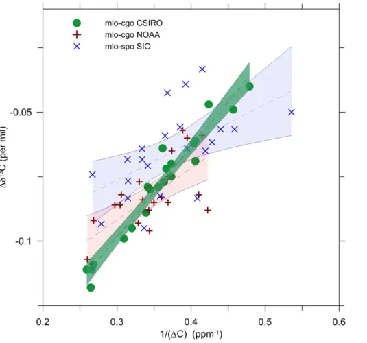
The CSIRO data in Fig. 2 reinforce the systematic nature of the _∆C variations with

5

a tight linear relationship between IH differences in the CO2 stable carbon isotope

ratio and in the inverse CO2 concentration, (∆C)− 1

, including both the step and pre-2010 year-to-year variations (r2=0.95). However inconsistency between laboratories, shown in Table 1, is substantial. Concentration data, particularly from CSIRO and NOAA (Masarie et al., 2001; Francey et al., 2015), are in sufficiently close agreement

10

that the differences must lie with isotopic measurement (Appendix B). The random na-ture of the scatter in Fig. 2 is emphasised by a lack of correlation between NOAA and SIO∆δ13C linear regression residuals (r2∼0.1).

We interpret the strong relationship using CSIRO isotope data as implying CO2

dom-inated by a C3 photosynthetic signature (Farquhar et al., 1982), including FF, but

ex-15

cluding significant contributions from oceans or equatorial C4 plants; also implied is that the CO2has had little opportunity for isotopic equilibration with natural reservoirs,

i.e.<1–2 years since release (Enting et al., 1995).

3 Reported source/sink anomalies

If ∆C variations in Fig. 1 are indeed systematic, then clues to the forcing should be

20

clarified by close examination of∆C and dC/dtat the times of a number of anomalous surface flux events that have been reported over the period.

The largest such events since the 1960s that influence CO2are the 1991 Pinatubo

volcanic eruption triggering increased removal of CO2 from the amosphere in

sub-sequent years (Frölicher et al., 2013) and 1997–1998 Indonesian peat fires (Page

(5)

BGD

12, 15087–15109, 2015

Title Page

Tables Figures

◭ ◮

Back Close

Full Screen / Esc

Discussion

P

a

per

|

Discussion

P

a

per

|

Discussion

P

a

per

|

Discussion

P

a

per

|

et al., 2009). Taking into account that the differences between NOAA and CSIRO mlo dC/dt records are smaller after 2000 (reflecting general improvements in measure-ment, Francey et al., 2015) the hemispheric differences during these two events are generally small, as expected if their influences are distributed into both hemispheres.

The major non-equatorial, terrestrial emission events reported over the last 2

5

decades are the 2002–2003 boreal wildfires (Giglio et a., 2013), the 2008 Global Fi-nancial Crisis (Peters et al., 2012) and 2011 SH savannah growth (Poulter et al., 2014):

– the 2002–2003 event corresponds to significant N–S differences in CO2 growth

rate, dC/dt, in Fig. 1b. Year 2003 corresponds to drought in Europe “un-precedented during the last century”, releasing∼0.5 Pg C yr−1(Ciais et al., 2005), 10

adding to 2003 GFED4 fire emissions in boreal America and boreal Asia of 0.3 Pg C,∼2 times the 1997–2013 mean (Giglio et al., 2013). However for

emis-sions spread evenly over a full year, a relatively small_∆C impact is expected since the 2003 NH FF combustion was ∼7.5 Pg C compared to <0.6 Pg C from NH

non-FF sources. Never-the-less 2002–2003 is, along with 2009–2010, a

consis-15

tent_∆C feature using the NOAA network data (Fig. S1). A possible IH exchange contribution is explored below.

– The Global Financial Crisis (GFC) of 2007–2008 coincides in Fig. 1b with the only occasion when the NH dC/dt ENSO peak is markedly smaller than that in the SH. While 2008, 2009 are the two lowest global fire emission years in the GFED4

20

database, combined boreal emissions are near average, favouring the GFC as a more likely explanation for the dC/dt behaviour. However, it is less clear that relatively low 2008, 2009∆C in Fig. 1a are attributable to the GFC, and a possible contribution from IH exchange is also examined below.

– The 2011 event was erroneously linked to “2010–2011”∆C changes by Poulter

25

(6)

BGD

12, 15087–15109, 2015

Title Page

Tables Figures

◭ ◮

Back Close

Full Screen / Esc

Discussion

P

a

per

|

Discussion

P

a

per

|

Discussion

P

a

per

|

Discussion

P

a

per

|

by around 6 months, a phase difference not observed for other significant El Niño peaks in Fig. 1b. This implies either an undetected NH source or changes in IH transport.

Independent evidence for the NH origin of the 2009 to 2010 CO₂∆C step comes from a recent analysis of upper troposphere measurements for 11 latitude bands between

5

30◦N to 30◦S (Matsueda et al., 2015) where the step is evident north of 10◦N. These authors suggest a role for transport, as well as source/sinks, to explain their year-to-year variations in latitudinal differences.

4 Anomalies in annual interhemispheric mixing

Meridional transport and eddy mixing due to large scale eddy motions are sources of

10

significant uncertainty in estimations of IH transport (Miyazaki et al., 2008). Here we examine the role of the opening and closing of the upper tropospheric equatorial west-erly duct, and associated inter-hemispheric Rossby wave propagation, as a contributor to the 2009–2010∆C_mlo-cgoshift, and other variations, shown in Fig. 1a.

Extra-tropical NH Rossby waves, including a branch of the Himalayan wave-train, are

15

able to penetrate into the SH when near-equatorial zonal winds are westerly in the up-per tropospheric duct centred on 140 to 170◦W and 5◦N to 5◦S (Webster and Holton, 1982; Frederiksen and Webster, 1988; Webster and Chang, 1988). This region is de-lineated and its tropospheric relevance revealed in Fig. 3a showing strongly correlated upper tropospheric westerly winds with the Southern Oscillation Index (SOI) over the

20

full 1949 to 2011 wind reanalysis dataset (http://www.esrl.noaa.gov/psd/data/gridded/ data.ncep.reanalysis.html).

The wind direction and strength (u_duct) in this duct are determined by seasonal and ENSO sea-surface temperature variations; the upper troposphere westerlies are strongest in the boreal winter, and during La Nina periods, when they are correlated

25

(7)

BGD

12, 15087–15109, 2015

Title Page

Tables Figures

◭ ◮

Back Close

Full Screen / Esc

Discussion

P

a

per

|

Discussion

P

a

per

|

Discussion

P

a

per

|

Discussion

P

a

per

|

other times, including El Ninos, theuductare near zero or easterly, causing the Rossby

wave eddies to be deflected northwards and dissipated in the equatorial regions, in-hibiting inter-hemispheric exchange.

For the period July 2009 to June 2010 the average 300 hPa equatorial zonal winds in the duct region were easterly as shown in Fig. 3c, effectively closing the duct and

5

increasing the build-up of FF CO2 in the NH. The July 2008 to June 2009 open duct

pattern, with westerlies in the duct, is shown in Fig. 3d. (Appendix C addresses the altitude range involved in this process. Note also, the meridional wind may make a small contribution to IH transport in the duct region during this time).

Figure 3b shows the 300 hPa zonal winds for July 2008 to June 2009 (Fig. 3d) minus

10

those for July 2009 to June 2010 (Fig. 3c) and the pattern bears strong similarities with the long-term zonal wind vs. SOI correlation in Fig. 3a.

5 Trace gas interhemispheric exchange through the duct

Inter-hemispheric exchange of a seasonally varying gas by this process depends on co-variance withuduct, and is represented in Fig. 4 by the product of monthlyuductand

15

∆C for routinely monitored CSIRO species C=CO2, CH4, CO and H2. The direction of

a step in∆C depends on the magnitude and sense of the trace gas IH gradient when the duct is open. The seasonality at mlo and cgo for the di_fferent gases are given in Fig. S2.

In the top panel monthly uduct are plotted over red and blue shading representing

20

El Niño and La Niña periods respectively. We add symbols connected by a solid line that are an integration of the NH winter peaks,Σuduct (October to April) for a nominal

uduct>2 ms− 1

, in order to better compare year-to-year changes in the strength and duration of the seasonal duct exchange.

Over the NH winters starting in 1995, 1997 and 2010 when Σuduct is <10 ms− 1

,

25

(8)

BGD

12, 15087–15109, 2015

Title Page

Tables Figures

◭ ◮

Back Close

Full Screen / Esc

Discussion

P

a

per

|

Discussion

P

a

per

|

Discussion

P

a

per

|

Discussion

P

a

per

|

by Giglio et al., 2013). The next lowest seasonally integratedΣuduct∼10 ms− 1

in 2003, has the next largest∆C increase (possibly complicating surface flux estimates from the inversion of CO₂spatial di_fferences by Rayner et al., 2008). For the next two occasions, whenΣuduct∼20 ms−

1

, there is no clear∆C response.

Compared to previous behaviour, the magnitude of exchange (∆C×uduct)

immedi-5

ately after the exended duct closure from July 2009 to June 2010 is the largest for each gas, in part reflecting the fact that 2010–2011 La Niña corresponds to the most intense

Σuductsince 1990 (top panel Fig. 4). The species exchange at this time is most marked

for CO₂and H₂, which we mainly attribute to the fact that these two gases exhibit the most significant∆C trend (CO2positive, H2negative) over the two decades; also each

10

has seasonal concentration amplitudes that are the largest compared to mean annual gradients (Fig. S2).

Through the four “duct-open” periods after 2010, Fig. 1a shows∆CO2 to be

prac-tically constant, a phenomena difficult to explain with known source/sink behaviour. During this periodΣu_ductmonitonically decreases; the constant∆C might be explained

15

if the decreasingΣuductare matched by decreases the annual fossil fuel emission

in-crements. Le Quere et al. (2014) estimate the annual increments in FF to be 0.5 Pg C in 2010, 0.3 Pg C in 2011 and 0.2 Pg C in 2012, supporting this interpretation.

6 Historic evidence for anomalous interhemispheric CO2exchange

Figure 5 examines the historic SIO mlo-spo records for responses to five other

ex-20

tended periods of duct-closure since the 1960s. Working backwards in time, there are seven occasions (circled in the top panel) when the seasonalΣuduct<5 ms−

1

. The five of these that correspond to an El Niño period closely followed by a La Niña (or in the case of 1982–1983 a weak La Niña shortly followed by a stronger one) show promi-nent peak values in∆C (circled bottom panel); the two lowΣuduct not coinciding with

25

(9)

BGD

12, 15087–15109, 2015

Title Page

Tables Figures

◭ ◮

Back Close

Full Screen / Esc

Discussion

P

a

per

|

Discussion

P

a

per

|

Discussion

P

a

per

|

Discussion

P

a

per

|

to missing data (particularly at spo) and measurement bias (Francey et al., 2015) and not considered further here. The 1986–1988 event most mirrors 2009–2010 being the next largest step, followed by four years of relatively stable∆C.

We conclude from this that anomalies in the inter-hemispheric exchange through the duct have played a significant ongoing role in modifying spatial differences in CO2

5

(and other trace species) at the surface. As NH FF CO2emissions increase further, the

influence is expected to become more marked in∆C×uduct.

7 Conclusions

Peylin et al. (2013) describe conflict between groups of models in locating the major global terrestrial sink, whether mid-northern latitude or equatorial, and suggest

atmo-10

spheric transport implementations may be involved. We have presented a variety of complementary evidence linking interhemispheric transport through the Pacific upper troposphere equatorial duct and the spatial and temporal difference in measured sur-face CO2 concentrations. The observed patterns of CO2 inter-hemispheric changes

are not easily explained by observed source/sink behaviour.

15

The observed 2009–2010 changes in CO₂ IH difference in particular, because of the magnitude and absence of plausible reported source/sink changes (in a time of unprecedented monitoring of ecosystem and ocean exchanges), provide an unusual opportunity to test the implementation of atmospheric transport in inversion models and help remove current ambiguities between surface exchanges and transport. More

20

(10)

BGD

12, 15087–15109, 2015

Title Page

Tables Figures

◭ ◮

Back Close

Full Screen / Esc

Discussion

P

a

per

|

Discussion

P

a

per

|

Discussion

P

a

per

|

Discussion

P

a

per

|

Appendix A: Trace gas data processing

The analyses for both dC/dt and ∆C are based on monthly average mixing ratios (or δ13C isotopic ratios) obtained from a smooth curve through individual flask data (typically 4 month−1_{) with combined harmonic (seasonal) and 80 day smoothing spline}

(Thoning et al., 1989). At Cape Grim, selected data represent strong near-surface

5

winds (>5 ms−1, 164 m a.s.l.) with trajectories (typically >10 days) over the South-ern Ocean; at Mauna Loa samples are collected in moderate down-slope winds; South Pole samples are selected to avoid local (station) contamination. Conventional smooth-ing splines through de-seasonalised baseline-selected concentration data, with 50 % attenuation at 22 months, are differentiated to provide dC/dt since 1992; Francey

10

et al. (2015) discuss dC/dt uncertainties. Annually averaged ∼80 day smoothed

monthly baseline concentration data are used to provide ∆C with near-annual time resolution, i.e. potential ambiguity between seasonality and inter-annual variation is addressed differently by dC/dtand∆C. CSIRO and NOAA data are processed identi-cally. Scripps data used here are monthly data that are seasonally adjusted and filled

15

(http://scrippsco2.ucsd.edu).

(Note: Using the spatial differences from individual laboratories effectively removes most calibration issues that can complicate high precision comparisons of data be-tween laboratories.) CO₂ differences between NOAA and CSIRO same-air compar-isons since 1992 are 0.11±0.13 ppm, with mean difference effectively cancelled in 20

mlo-cgo comparisons. This means the maximumδ13C measurement error due to CO2

difference should be less than 0.005 ‰.

Appendix B: Laboratory differences inδ13_{C data}

A linear regression between ∆δ13C and ∆C for the pre-2010 CSIRO mlo-cgo data gives:∆δ13C=0.050(±0.004)×∆C+0.062,r2=0.92 with slope 0.05 ‰×ppm−1 char-25

(11)

BGD

12, 15087–15109, 2015

Title Page

Tables Figures

◭ ◮

Back Close

Full Screen / Esc

Discussion

P

a

per

|

Discussion

P

a

per

|

Discussion

P

a

per

|

Discussion

P

a

per

|

−18 ‰ with respect to air, while C4 plant fractionation is ∼ −7 ‰ and fractionation for

CO2entering the ocean is small∼ −2 ‰). Over the whole period the slope reduces to

0.41 due to non-linearity exposed by the 0.8 ppm step. Using (∆C)−1in Fig. 2 gives the slope 0.342(±0.057) ‰ ppm pre-2010 and 0.350(±0.018) ‰ ppm overall.

Exact reasons for the varying quality of δ13C programs in Fig. 2 are not known.

5

However, reduced scatter in CSIRO program (Allison and Francey, 2007) is possibly related to feedback from regular quality assessment provided by unique method redun-dancy; the data in this report involve small subsamples of chemically dried whole flask air, from which CO2 is extracted and analysed using a fully automated Finnigan-Matt

602 D Mass Spectrometer (MS) with MT Box-C extraction accessory, and bracketed

10

by extractions and analysis of cgo long-lived baseline air standards in high-pressure cylinders. Over most of the two decades a parallel cgo program involved unique large-sample in situ extraction of CO2, which is returned and analysed on the same MS, but

relative to independently propagated pure CO₂ standards. Unfortunately, substantial reduction in support means continuing quality of the CSIRO program is not assured

15

from 2014 (2014 data not included).

Appendix C: Atmospheric transport

In contrast to the situation in Fig. 3c, the average 300 hPa zonal wind for July 2008 to June 2009, shown in Fig. 3d, has equatorial westerlies between the date line and 120 W. The westerly duct is open and NH extra-tropical Rossby waves, including the

20

Himalayan wave-train, are able to penetrate into the SH. Correlation analysis (Fred-eriksen and Webster, 1988) indicates increased upper tropospheric transient kinetic energy near the equator with facilitated IH transport of trace gases. Here we have fo-cused on the 300 hPa level, but our results apply in broad terms to most of the upper troposphere. In particular, the correlation of the SOI with the zonal wind in the

west-25

(12)

BGD

12, 15087–15109, 2015

Title Page

Tables Figures

◭ ◮

Back Close

Full Screen / Esc

Discussion

P

a

per

|

Discussion

P

a

per

|

Discussion

P

a

per

|

Discussion

P

a

per

|

(July 2008 to June 2009) minus (July 2009 to June 2010) zonal wind difference (Fig. 3b) is largely equivalent barotropic with similar strength between 300 and 100 hPa and re-ducing at the upper and lower levels. Northern winter (DJF) differences for 2008/09 minus 2009/10 are circa twice as strong in the westerly duct region as those in Fig. 3b.

The Supplement related to this article is available online at 5

doi:10.5194/bgd-12-15087-2015-supplement.

Author contributions. R. J. Francey provided trace gas information and J. S. Frederiksen the atmospheric dynamics information.

Acknowledgements. This paper relies on the decades-long commitment by skilled CSIRO GASLAB scientific personnel, particularly Paul Steele, Ray Langenfelds, Paul Krummel, Colin 10

Allison, Paul Fraser and Marcel van der Schoot; many support sta_ffin GASLAB, Cape Grim Baseline Air Pollution Station (The Australian Bureau of Meteorology with CSIRO), and mea-surement collaborators at NOAA, also contribute directly in this regard. The importance of the historic SIO records cannot be understated. Rachel Law provided global, and Ying Ping Wang with Chris Lu regional, CO₂modelling advice.

15

References

Ashfold, M. J., Pyle, J. A., Robinson, A. D., Meneguz, E., Nadzir, M. S. M., Phang, S. M., Samah, A. A., Ong, S., Ung, H. E., Peng, L. K., Yong, S. E., and Harris, N. R. P.: Rapid transport of East Asian pollution to the deep tropics, Atmos. Chem. Phys., 15, 3565–3573, doi:10.5194/acp-15-3565-2015, 2015.

20

Ciais, Ph., Reichstein, M., Viovy, N., Granier, A., Ogée, J., Allard, V., Aubinet, M., Buchmann, N., Bernhofer, Chr., Carrara, A., Chevallier, F., De Noblet, N., Friend, A. D., Friedlingstein, P., Grünwald, T., Heinesch, B., Keronen, P., Knohl, A., Krinner, G., Loustau, D., Manca, G., Matteucci, G., Miglietta, F., Ourcival, J. M., Papale, D., Pilegaard, K., Rambal, S., Seufert, G., Soussana, J. F., Sanz, M. J., Schulze, E. D., Vesala, T., and Valentini, R.: Europe-wide reduc-25

(13)

BGD

12, 15087–15109, 2015

Title Page

Tables Figures

◭ ◮

Back Close

Full Screen / Esc

Discussion

P

a

per

|

Discussion

P

a

per

|

Discussion

P

a

per

|

Discussion

P

a

per

|

Dlugokencky, E. J., Lang, P. M., Masarie, K. A., Crotwell, A. M., and Crotwell, M. J.: Atmospheric Carbon Dioxide Dry Air Mole Fractions from the NOAA ESRL Carbon Cycle Cooperative Global Air Sampling Network, 1968–2013, Version: 2014-06-27, available at: ftp://aftp.cmdl. noaa.gov/data/trace_gases/co2/flask/surface/ (last access: January 2015), 2014.

Enting, I. G., Trudinger, C. M., and Francey, R. J.: A synthesis inversion of the concentration 5

andδ13C of atmospheric CO₂, Tellus B, 47, 35–52, 1995.

Farquhar, G. D., O’Leary, M. H., and Berry, J. A.: On the relationship between carbon isotope discrimination and the intercellular carbon dioxide concentration in leaves, Aust. J. Plant Physiol., 9, 121–137, 1982.

Francey, R. J., Trudinger, C. M., van der Schoot, M., Law, R. M., Krummel, P. B., Langen-10

felds, R. L., Steele, L. P., Allison, C. E., Stavert, A. R., Andres, R. J.m and Rödenbeck, C.: Atmospheric verification of anthropogenic CO₂emission trends, Nature Climate Change, 3, 520–524, doi:10.1038/nclimate1817, 2013.

Francey, R. J., Langenfelds, R. L., Steele, L. P., Krummel, P. B., and van der Schoot, M.: Bias in the biggest terms in the global carbon budget?, in: Baseline Atmospheric Program Australia 15

2011–2013, edited by: Krummel, P. B. and Derek, N., Australian Bureau of Meteorology in cooperation with CSIRO Division of Atmospheric Research, Melbourne, in press, 2015. Frederiksen, J. S. and Webster, P. J.: Alternative theories of atmospheric teleconnections and

low-frequency fluctuations, Rev. Geophys., 26, 459–494, 1988.

Frölicher, T. L., Joos, F., Raible, C. C., and Sarmiento, J. L.: Atmospheric CO₂ response to 20

volcanic eruptions: the role of ENSO, season, and variability, Global Biogeochem. Cy. 27, 239–251, doi:10.1002/gbc.20028, 2013.

Giglio, L., Randerson, J. T., and van derWerf, G. R.: Analysis of daily, monthly, and annual burned area using the fourth-generation global fire emissions database (GFED4),http://www. falw.vu/~gwerf/GFED/GFED4/tables/GFED4.1s_CO2.txt (last access: September 2015), J. 25

Geophys. Res.-Biogeo., 118, 317–328, doi:10.1002/jgrg.20042, 2013.

Keeling, R. F., Piper, S. C., Bollenbacher, A. F., and Walker, J. S.: Atmospheric CO₂ records from sites in the SIO air sampling network. In Trends: a Compendium of Data on Global Change. Carbon Dioxide Information Analysis Center, Oak Ridge National Laboratory, U.S. Department of Energy, Oak Ridge, Tenn., USA, doi:10.3334/CDIAC/atg.035, 2009.

30

(14)

BGD

12, 15087–15109, 2015

Title Page

Tables Figures

◭ ◮

Back Close

Full Screen / Esc

Discussion

P

a

per

|

Discussion

P

a

per

|

Discussion

P

a

per

|

Discussion

P

a

per

|

Jain, A. K., Johannessen, T., Kato, E., Keeling, R. F., Kitidis, V., Klein Goldewijk, K., Koven, C., Landa, C. S., Landschützer, P., Lenton, A., Lima, I. D., Marland, G., Mathis, J. T., Metzl, N., Nojiri, Y., Olsen, A., Ono, T., Peng, S., Peters, W., Pfeil, B., Poulter, B., Raupach, M. R., Regnier, P., Rödenbeck, C., Saito, S., Salisbury, J. E., Schuster, U., Schwinger, J., Séférian, R., Segschneider, J., Steinhoff, T., Stocker, B. D., Sutton, A. J., Takahashi, T., Tilbrook, B., 5

van der Werf, G. R., Viovy, N., Wang, Y.-P., Wanninkhof, R., Wiltshire, A., and Zeng, N.: Global carbon budget 2014, Earth Syst. Sci. Data, 7, 47–85, doi:10.5194/essd-7-47-2015, 2015.

Locatelli, R., Bousquet, P., Chevallier, F., Fortems-Cheney, A., Szopa, S., Saunois, M., Agusti-Panareda, A., Bergmann, D., Bian, H., Cameron-Smith, P., Chipperfield, M. P., Gloor, E., 10

Houweling, S., Kawa, S. R., Krol, M., Patra, P. K., Prinn, R. G., Rigby, M., Saito, R., and Wilson, C.: Impact of transport model errors on the global and regional methane emissions estimated by inverse modelling, Atmos. Chem. Phys., 13, 9917–9937, doi:10.5194/acp-13-9917-2013, 2013.

Masarie, K. A., Langenfelds, R. L., Allison, C. E., Conway, T. J., Dlugokencky, E. J., 15

Francey, R. J., Novelli, P. C., Steele, L. P., Tans, P. P., Vaughn, B., and White, J. W. C.: NOAA/CSIRO Flask Air Intercomparison Experiment: a strategy for directly assessing con-sistency among atmospheric measurements made by independent laboratories. J. Geophys. Res., 106, 20445–20464, 2001.

Matsueda, H., Machida, T., Sawa, Y., and Niwa, Y.: Long-term change of CO₂ lat-20

itudinal distribution in the upper troposphere, Geophys. Res. Lett., 42, 2508–2514, doi:10.1002/2014GL062768, 2015.

Miyazaki, K., Patra, P. K., Takigawa, M., Iwasaki, T., and Nakazawa, T.: Global-scale transport of carbon dioxide in the troposphere, J. Geophys. Res., 113, D15, doi:10.1029/2007JD009557, 2008.

25

Page, S. E., Hoscilo, Langner, A., A., Tansey, K. J., Siegert, F., Limin, S. H., and Rieley, J. O.: Tropical peatland fires in Southeast Asia, in: Tropical Fire Ecology: Climate Change, Land Use and Ecosystem Dynamics, edited by: Cochrane, M. A., Springer-Praxis, Heidelberg, Germany, 263–287, 2009.

Poulter, B., Frank, D., Ciais, P., Myneni, R. B., Andela, N., Bi, J., Broquet, G., Canadell, J. G., 30

(15)

BGD

12, 15087–15109, 2015

Title Page

Tables Figures

◭ ◮

Back Close

Full Screen / Esc

Discussion

P

a

per

|

Discussion

P

a

per

|

Discussion

P

a

per

|

Discussion

P

a

per

|

Rayner, P. J., Law, R. M., Allison, C. E., Francey, R. J., Trudinger, C. M., and Pickett-Heaps, C.: Interannual variability of the global carbon cycle (1992–2005) inferred by inver-sion of atmospheric CO₂andδ13CO₂measurements, Global Biogeochem. Cy., 22, GB3008, doi:10.1029/2007GB003068, 2008.

Stephens, B. B., Gurney, K. R., Tans, P. P., Sweeney, C., Peters, W., Bruhwiler, L., Ciais, P., 5

Ramonet, M. l. Bousquet, P., Nakazawa, T., Aoki, S., Machida, T., Inoue, G., Vinnichenko, N., Lloyd, J. Jordan, A., Heimann, M., Shibistova, O. , Langenfelds, R. L., Steele, L. P., Francey, R. J., and Denning, A. S., Weak Northern and Strong Tropical Land Carbon Uptake from Vertical Profiles of Atmospheric CO₂, Science, 316, 1732–1735, 2007.

Thoning, K. W., Tans, P. P., and Komhyr, W. D.: Atmospheric carbon dioxide at Mauna Loa 10

observatory, 2, Analysis of the NOAA/GMCC data, 1974–1985, J. Geophys. Res., 94, 8549– 8565, 1989.

Webster, P. J. and Chang, H.-R.: Equatorial energy accumulation and emanation regions: im-pacts of a zonally varying basic state, J. Atmos. Sci., 45, 803–829, 1988.

Webster, P. J. and Holton, J. R.: Cross-equatorial response to mid-latitude forcing in a zonally 15

(16)

BGD

12, 15087–15109, 2015

Title Page

Tables Figures

◭ ◮

Back Close

Full Screen / Esc

Discussion

P

a

per

|

Discussion

P

a

per

|

Discussion

P

a

per

|

Discussion

P

a

per

|

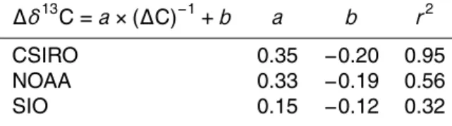
Table 1.Coefficients in linear regressions between the annual mean CO₂stable isotope diff er-ence and the inverse of the annual mean CO₂concentration difference between mlo and either cgo (CSIRO, NOAA) or spo (SIO).

∆δ13C=a_×(∆C)−1+b a b r2

CSIRO 0.35 ₋0.20 0.95

NOAA 0.33 ₋0.19 0.56

(17)

BGD

12, 15087–15109, 2015

Title Page

Tables Figures

◭ ◮

Back Close

Full Screen / Esc

Discussion

P

a

per

|

Discussion

P

a

per

|

Discussion

P

a

per

|

Discussion

P

a

per

(18)

BGD

12, 15087–15109, 2015

Title Page

Tables Figures

◭ ◮

Back Close

Full Screen / Esc

Discussion

P

a

per

|

Discussion

P

a

per

|

Discussion

P

a

per

|

Discussion

P

a

per

|

(19)

BGD

12, 15087–15109, 2015

Title Page

Tables Figures

◭ ◮

Back Close

Full Screen / Esc

Discussion

P

a

per

|

Discussion

P

a

per

|

Discussion

P

a

per

|

Discussion

P

a

per

|

(20)

BGD

12, 15087–15109, 2015

Title Page

Tables Figures

◭ ◮

Back Close

Full Screen / Esc

Discussion

P

a

per

|

Discussion

P

a

per

|

Discussion

P

a

per

|

Discussion

P

a

per

(21)

BGD

12, 15087–15109, 2015

Title Page

Tables Figures

◭ ◮

Back Close

Full Screen / Esc

Discussion

P

a

per

|

Discussion

P

a

per

|

Discussion

P

a

per

|

Discussion

P

a

per

|

(22)

BGD

12, 15087–15109, 2015

Title Page

Tables Figures

◭ ◮

Back Close

Full Screen / Esc

Discussion

P

a

per

|

Discussion

P

a

per

|

Discussion

P

a

per

|

Discussion

P

a

per

|

(23)

BGD

12, 15087–15109, 2015

Title Page

Tables Figures

◭ ◮

Back Close

Full Screen / Esc

Discussion

P

a

per

|

Discussion

P

a

per

|

Discussion

P

a

per

|

Discussion

P

a

per

|