Refinamento de malha superficial baseado na aproximação suave da superficie do modelo

(1)

Programa de Pós-Gradua¸cão em Engenharia Elétrica

Refinamento de Malha Superficial Baseado na

Aproxima¸c˜

ao Suave da Superf´ıcie do Modelo

C´

assia Regina Santos Nunes

Orientador: Prof. Dr. Renato Cardoso Mesquita (UFMG)

Co-Orientador: Prof. Ph.D. David Alister Lowther (McGill University)

Tese apresentada ao Curso de Pós-Gradua¸cão em Enge-nharia Elétrica da Universidade Federal de Minas Ge-rais, como requisito parcial para obten¸cão do t´ıtulo de Doutor em Engenharia Elétrica.

(2)

Programa de Pós-Gradua¸cão em Engenharia Elétrica

Remeshing Driven by Smooth Approximation

of Model Surface

C´

assia Regina Santos Nunes

Advisor: Prof. Dr. Renato Cardoso Mesquita (UFMG)

Co-Advisor: Prof. Ph.D. David Alister Lowther (McGill University)

Thesis presented to the Graduate Program in Electrical Engineer of the Federal University of Minas Gerais in partial fulfillment of the requirements for the degree of Doctor in Electrical Engineer.

(3)

To my parents, Sebasti˜ao Daniel e Maria F´atima, my first masters.

(4)

Ao professor Renato Cardoso Mesquita por ter compartilhado comigo grandes id´eias

e permitido que eu realizasse este trabalho. Sua paciˆencia, disponibilidade e exigˆencia

foram essenciais para o meu crescimento intelectual e pessoal.

`

As minhas queridas irmãs, Danielle Fátima e Maria Cláudia, pelo carinho e incentivo.

Aos alunos de inicia¸c˜ao cient´ıfica, em especial, Felipe Terra e Raphael Chaves, pelo

empenho na execu¸c˜ao deste trabalho.

Aos professores Jaime Arturo Ram´ırez, Rodney Rezende Saldanha e Elson Jos´e da

Silva pelos ensinamentos e aux´ılios para apresenta¸c˜oes de trabalhos em Congressos.

Aos colegas do GOPAC Ricardo, Alexandre, Douglas e Luciano pelas brincadeiras e

ajuda na solu¸c˜ao de problemas.

Aos colegas de caminhada, Lane, Carla, Marcelo, Anderson, Jose Hissa, Ademir, Julio

e Elizabeth pelas trocas de exper´ıências e conversas agradáveis na hora do café.

Ao meu amigo, Frederico Bruno Ribas Soares, pelas palavras reconfortantes e

incen-tivadoras.

`

As minhas amigas Larissa, Ma´ıra, Ana Paula e Let´ıcia pelas nossas conversas

inter-min´aveis sobre tudo.

Ao Geraldo, meu osteopata, fisioterapeuta, acupunturista e grande amigo.

Aos mestrandos, doutorandos, professores e funcion´arios do CPDEE/UFMG pela

convivˆencia e coopera¸c˜ao.

(5)

`

A CAPES, pela bolsa de estudos durante a realiza¸c˜ao deste trabalho.

`

A CAPES/PDEE, pela concess˜ao da bolsa de doutorado sandu´ıche para a McGill

(6)

I would like to also thank professor David Alister Lowther for receiving me and

coa-ching me during my stay in Montreal/Canad´a.

Many thanks to my CADLAB/McGill friends, Dileep Nair and Linda Wang, for

sharing amazing moments with me.

Thanks a lot to Kate, Sue, Gustavo, Nadia, Marcia and, specially, Raquel for been

my family when I was in Montreal.

(7)

O m´etodo de elementos finitos ´e uma poderosa ferramenta para a comunidade de

engenharia. Uma das barreiras para automatiza¸cão de análises pelo método de

elemen-tos finielemen-tos é a gera¸cão automática de malhas de boa qualidade. Uma malha com boa

distribui¸cão de nós e elementos bem formados contribui na gera¸cão de sistemas bem

con-dicionados, minimizando erros num´ericos e singularidades. Contudo, a maioria das malhas

não é considerada satisfatória sem a aplica¸cão de alguma etapa de pós-processamento para

melhorar suas propriedades. As malhas que representam modelos resultantes da

aplica-¸cão das opera¸cões Booleanas e de montagem à modelos pré-existentes possuem um grande

n´umero de elementos mal formados. O problema de baixa qualidade tamb´em ocorre em

malhas geradas por t´ecnicas de reconstru¸c˜ao de superf´ıcies.

Este trabalho apresenta um algoritmo efetivo de refinamento de malhas superficiais

para melhorar a forma dos elementos, a distribui¸c˜ao nodal e suas conex˜oes. Este processo

consiste na aplica¸cão de séries de operadores de modifica¸cão local para: mover, retirar

e inserir n´os na malha superficial. Para evitar a perda das caracter´ısticas geom´etricas

do modelo, uma nova técnica de aproxima¸cão da geometria é apresentada. Como, na

maioria das vezes, apenas a configura¸cão da malha é conhecida, a aproxima¸cão suave do

modelo é calculada por partes a partir dos nós que compõem a malha. Os movimentos

dos nós são direcionados pela aproxima¸cão, o que assegura que eles permane¸cam sobre a

superf´ıcie original durante o aprimoramento da malha. Alguns exemplos s˜ao apresentados

para ilustrar os resultados alcan¸cados ap´os a aplica¸c˜ao do nosso esquema de refinamento

da malha.

(8)

The finite element method is a powerful tool for the engineering community. One of

the barriers for automating finite element analysis is the automatic generation of

high-quality meshes. Meshes with good nodes distribution and well-shaped elements provides

good system conditioning, which minimizes errors and singularities that might arise.

How-ever, most meshes can hardly be called satisfactory without any kind of post-processing

to improve their qualities. The meshes representing models generated by the application

of the Boolean and assembly operations to predefined primitives have a large number

of badly shaped elements. The quality problem also raises in models obtained by the

acquisition process, like scanning devices.

This work presents an effective remeshing algorithm to improve the shape,

distribu-tion and connectivity of the surface mesh elements, while keeping the mesh geometrically

close to the model surface. Our post-processing scheme applies series of local mesh

modi-fications operators to the input mesh. The local operators are able to improve, refine and

simplify the mesh. To ensure fidelity, a novel technique was developed to approximate

the model surface by smooth surface patches. Since, most of the time, only the mesh

configuration is available, a smooth surface approximation is evaluated by pieces from the

mesh nodes. The approximation is used to drive the nodes movements and assure that

they stay on top of the original model surface during the application of the local mesh

modifications. Many examples are presented to illustrate the accomplished results of this

work.

(9)

O texto a seguir consiste em um resumo estendido sobre o trabalho desenvolvido nesta

tese. Primeiramente, este texto introduz o problema abordado, a principal motiva¸c˜ao

para solucion´a-lo e alguns dos principais m´etodos relacionados. Em seguida, uma breve

descri¸cão da principal metodologia desenvolvida é apresentada. Finalmente, as conclusões

s˜ao apresentadas.

Introdu¸c˜

ao

O método de elementos finitos (FEM - Finite Element Method) é uma boa escolha para solucionar equa¸cões diferenciais parciais (PDEs - Partial Differential Equations) em dom´ınios complexos. FEM aproxima numericamente a solu¸cão de PDEs lineares e

não-lineares pela substitui¸cão do sistema cont´ınuo de equa¸cões por um número finito

de equa¸cões algébricas lineares e não-lineares acopladas. O dom´ınio do problema deve

ser dividido em partes menores de forma simples, construindo uma malha de elementos

finitos. Esta malha deve aproximar o dom´ınio de estudo e seus elementos devem satisfazer

restri¸c˜oes de tamanho e forma.

Em an´alise pelo FEM, a qualidade da aproxima¸c˜ao da superf´ıcie e a qualidade da

forma dos elementos da malha volumétrica afetam a precisão dos resultados numéricos.

Por exemplo, se os ângulos internos dos elementos são próximos a 180◦_{, o erro de}

dis-cretiza¸cão da solu¸cão aumenta; se os ângulos são próximos a zero, o número de condi¸cão

da matriz do elemento aumenta. Resumindo, uma malha com boa distribui¸c˜ao de n´os

e elementos bem formados contribui na gera¸c˜ao de sistemas bem condicionados, o que

(10)

minimiza erros num´ericos e singularidades que possam ocorrer.

A qualidade da malha volumétrica está intimamente ligada à qualidade da malha

superficial. Uma malha superficial de baixa qualidade pode inviabilizar a gera¸c˜ao da

malha volum´etrica correspondente, ou os elementos obtidos s˜ao de baixa qualidade. Em

geral, os programas geradores de malhas volum´etricas tˆem autonomia para inserir novos

pontos na malha superficial, mas n˜ao podem decidir sobre a retirada ou modifica¸c˜ao da

localiza¸c˜ao de um v´ertice da malha inicial. A malha superficial inicial deve estar presente

na malha volum´etrica resultante. Assim, malhas superficiais de boa qualidade facilitam a

obten¸cão de malhas volumétricas também de boa qualidade.

A princ´ıpio, modeladores de s´olidos podem produzir malhas superficiais de alta

qua-lidade, mas após a aplica¸cão de algumas opera¸cões Booleanas e de opera¸cões montagem

a modelos pr´e-existentes, a qualidade da malha resultante diminui drasticamente. O

pro-blema de baixa qualidade também ocorre em malhas geradas por técnicas de reconstru¸cão

de superf´ıcies. Estas t´ecnicas reconstroem superf´ıcies a partir de um conjunto de pontos,

os quais podem ser obtidos de v´arios tipos de fontes, como digitalizadores tridimensionais

a laser. As técnicas de reconstru¸cão enfatizam a aproxima¸cão da geometria e topologia,

mas n˜ao garantem a qualidade da malha superficial gerada.

Neste contexto, refinar a malha superficial torna-se muito importante para

maximi-zar a qualidade da forma de seus elementos, reduzindo o n´umero de ˆangulos agudos,

melhorando a distribui¸c˜ao nodal e suas conex˜oes.

O objetivo deste projeto ´e a gera¸c˜ao de malhas superficiais de alta qualidade para

modelos obtidos atrav´es de processos de aquisi¸c˜ao de dados ou modelos resultantes da

aplica¸cão das opera¸cões Booleanas e/ou de montagem sobre primitivas pré-definidas. Uma

malha de alta qualidade viabiliza um sistema de elementos finitos bem condicionado, o

que aumenta a precis˜ao dos resultados obtidos.

Para melhorar a qualidade da malha superficial, diferentes m´etodos de p´os-processamento

podem ser usados. Existem três técnicas básicas para melhoramento da malha: suaviza¸cão

(smoothing), simplifica¸cão (clean-up) e subdivisão (refining). Suaviza¸cão inclui qualquer método que melhora o posicionamento dos nós sem alterar suas conexões. Simplifica¸cão,

geralmente, refere-se a processos que modificam a conectividade dos elementos, atrav´es da

(11)

inserindo novos elementos. Na maioria das vezes, a aplica¸c˜ao de apenas uma dessas

téc-nicas não é suficiente para alcan¸car o n´ıvel de qualidade desejado. Então, para garantir a

obten¸cão de uma malha superficial com alto grau de qualidade, duas ou três técnicas são

aplicadas em conjunto, o que gera m´etodos h´ıbridos de p´os-processamento.

Em outra classifica¸cão, os métodos de refinamento de malhas superficiais são divididos

em três grupos. O primeiro grupo é baseado no particionamento das malhas 3D em pat-ches(partes) e no tratamento de cada parte em separado. Esta técnica produz resultados razoáveis, mas é muito sens´ıvel a estrutura dospatches, além da amostragem dos vértices ser de dif´ıcil controle. Outro grupo de algoritmos está baseado na parametriza¸cão global

da malha original. Uma nova triangula¸c˜ao de boa qualidade ´e gerada sobre o dom´ınio

param´etrico e depois projetada de volta ao espa¸co 3D. Assim, a malha resultante ´e uma

vers˜ao melhorada do modelo original. A principal desvantagem dos m´etodos de

para-metriza¸cão global é a sensibilidade dos resultados à parapara-metriza¸cão utilizada. Converter

uma estrutura 3D n˜ao-trivial num plano param´etrico distorce drasticamente a estrutura

e informa¸c˜oes importantes, n˜ao especificadas claramente, podem ser perdidas. Mesmo

que a parametriza¸cão minimize as distor¸cões do modelo original, é imposs´ıvel eliminá-las

completamente. Além disso, os métodos de cálculo da parametriza¸cão global são lentos,

pois eles envolvem a solu¸cão de grandes sistemas de equa¸cões, muitas vezes não-lineares.

A principal alternativa à parametriza¸cão global é trabalhar diretamente sobre a malha

superficial e realizar s´eries de modifica¸c˜oes locais para melhorar, enriquecer ou simplificar

a malha. Está técnica é conhecida como processo de adapta¸cão da malha ou simplesmente

remeshing(refinamento da malha) e este método é utilizado neste trabalho. Algoritmos de remeshing podem ser considerados métodos h´ıbridos, pois os operadores de modifica¸cão local da malha encapsulam as técnicas básicas de suaviza¸cão, simplifica¸cão e subdivisão.

Os operadores de modifica¸c˜oes locais permitem mover, retirar e inserir n´os na malha

superficial. Para evitar a perda das caracter´ısticas geom´etricas do modelo, torna-se

es-sencial o uso de uma aproxima¸c˜ao da geometria do modelo. Essa aproxima¸c˜ao direciona

os movimentos dos n´os e assegura que eles permane¸cam sobre a superf´ıcie original do

modelo.

Infelizmente, na maioria das vezes, apenas a configura¸cão da malha é conhecida e não

as caracter´ısticas geom´etricas do modelo. Para superar este problema, uma representa¸c˜ao

(12)

aproxima-¸cão geométrica é calculada por partes a partir dos vértices que compõem a malha. Os

operadores de modifica¸cões locais são aplicados à malha, levando em considera¸cão as

infor-ma¸cões geométricas provenientes da aproxima¸cão da superf´ıcie do modelo. A constru¸cão

da representa¸c˜ao suave da superf´ıcie do modelo constitui na principal contribui¸c˜ao deste

trabalho.

A próxima se¸cão apresenta a técnica introduzida para o cálculo da aproxima¸cão suave

da superf´ıcie do modelo. Em seguida, o m´etodo para refinamento de malhas superficiais

utilizando esta t´ecnica ´e discutido.

Aproxima¸c˜

ao Suave da Superf´ıcie do Modelo

A aproxima¸c˜ao da superf´ıcie do modelo ´e muito importante durante o processo de

refinamento da malha superficial. É através dela que as caracter´ısticas geométricas do

modelo ser˜ao conhecidas e preservadas. Um operador de modifica¸c˜ao local da malha

´e aplicado apenas quando a qualidade da forma do elemento e o erro de aproxima¸c˜ao

permanecem dentro dos limites pr´e-estabelecidos.

A aproxima¸cão utilizada deve garantir a representa¸cão de modelos gerados através da

aplica¸cão das opera¸cões Booleanas e opera¸cão de montagem sobre primitivas pré-definidas,

assim como de modelos gerados a partir de t´ecnicas de reconstru¸c˜ao de superf´ıcies. Por

defini¸c˜ao, os modelos reconstru´ıdos s˜ao obtidos a partir de um conjunto desorganizado

de pontos P, usualmente denso, amostrados diretamente de uma superf´ıcie suave S. Por

outro lado, as malha resultantes das aplica¸c˜oes das opera¸c˜oes Booleanas e de montagem

podem ser formadas por superf´ıcies planares e curvas. Seu conjunto de v´ertices ´e

normal-mente reduzido. Para representar os dois tipos de modelos, a t´ecnica de aproxima¸c˜ao da

superf´ıcie do modelo por um conjunto de patches(partes) suaves é introduzida. A cada face da malha é associado um patch suave, que pode ser plano ou curvo. Aproximar a geometria do modelo por um conjunto de patches diminui o tempo de processamento e minimiza erros de aproxima¸cão, pois a parametriza¸cão global é evitada.

Para calcular a aproxima¸c˜ao de uma face da malha, os v´ertices da mesma e os

vér-tices vizinhos são utilizados. O uso dos vérvér-tices vizinhos é importante para melhorar a

(13)

lo-cal do modelo. Se o conjunto de vértices é coplanar, a aproxima¸cão da face é um patch plano; senão, a face é aproximada por um patch curvo. Outro aspecto considerado na identifica¸cão do tipo depatch é o erro associado à aproxima¸cão calculada. Após o cálculo dopatch curvo, o erro médio entre o patch e os vértices utilizado no cálculo é avaliado. Se o erro for maior que um valor limite especificado (por exemplo: o erro máximo pode ser

limitado em 2%), a aproxima¸cão é descartada e a face é então aproximada por um plano.

A aproxima¸cão de toda a superf´ıcie do modelo é formada por um conjunto de patches suaves curvos ou planos. Os patches curvos são patches B-splines calculados através da técnica de m´ınimos quadrados, onde os vértices da face a ser aproximada e seus vértices

vizinhos s˜ao as entradas.

As superf´ıcies param´etricas B-splines s˜ao frequentemente usadas em sistemas CAD

(Computer Aided Design - Projeto Assistido por Computador) para aproximar pontos distribu´ıdos irregularmente no espa¸co. Entre as vantagens na utiliza¸c˜ao das B-splines,

destacam-se: i) garantia de boa aproxima¸c˜ao de uma grande variedade de s´olidos; ii)

preserva¸c˜ao de altos graus de continuidade em superf´ıcies complexas; e iii) controle local,

o que significa que uma modifica¸cão local da forma não é propagada para toda a superf´ıcie.

O problema consiste em encontrar um patch de superf´ıcie B-spline s(u, v), que apro-xima um conjunto de v´ertices, com representa¸c˜ao da forma:

s(u, v) =

ν X

ω=0

Mω(u, v)cω, (1)

onde,cω são pontos de controle eMω(u, v) são fun¸cões base.

Seja pτ,τ = 1, ..., µ, o conjunto de v´ertices da face e seus v´erticies vizinhos e sτ suas

aproxima¸cões. A aproxima¸cão é calculada como um m´ınimo da fun¸cãoF:

F =

µ X

τ=0

ks(uτ, vτ)−pτk

2 = µ X τ=0 " _ν X ω=0

Mω(uτ, vτ)cω−pτ #2

. (2)

Ou seja, assumindo que as fun¸cões base, Mω, são dadas ou pré-calculadas, precisa-se

encontrar o conjunto de pontos de controle, cω, que minimize F.

Este problema clássico de aproxima¸cão por m´ınimos quadrados sempre possui solu¸cão.

(14)

ser suficientemente suave. Por isso, acrescenta-se à Equa¸cão 2 um termo quadrático de

regulariza¸c˜ao (Fs), denominado termo de suaviza¸c˜ao ou termo de penalidade. Assim,

garante-se que a solu¸cão seja única e com suaviza¸cão controlada. Frequentemente, esse

termo é obtido a partir da aproxima¸cão dethin-plate energy, uma fun¸cão quadrática nas derivadas parciais de segunda ordem:

Fs = Z Z

(s2

uu+ 2s

2

uv+s

2

vv)dudv. (3)

ou a partir de membrane energy que ´e quadr´atica nas derivadas parciais de primeira ordem:

Fs = Z Z

(s2

u+s

2

v)dudv. (4)

Acrescentando o termo de suaviza¸cão a Equa¸cão 2, a fun¸cão a ser minimizada torna-se:

F = µ X τ=0 " _ν X ω=0

Mω(uτ, vτ)cω−pτ #2

+λFs, (5)

ondeλé um valor real maior ou igual a zero, denominado parâmetro de suaviza¸cão. Como

F e qualquer um dos termos de suaviza¸cão (Fs) são quadráticos em cω, a Equa¸cão 5 pode

ser reescrita na forma matricial:

F=_kBc₋p_k2₂+λcTEc, (6)

onde, c = (c1, ..., cν)T, p = (p1, ..., pµ)T, E ´e uma matriz ν × ν, sim´etrica e definida

positiva, e a matriz B´eµ_×ν, da forma:

B =        

M1(u1, v1) . . . Mν(u1, v1)

M1(u2, v2) . . . Mν(u2, v2)

... . . . ...

M1(uµ, vµ) . . . Mν(uµ, vµ)         (7)

Tomando-se o gradiente de F e igualando-o a zero, tem-se:

(15)

A matriz BT_B _{´e de ordem} _n

×n, simétrica e semi-definida positiva, então a solu¸cão da Equa¸cão 8 com λ = 0 não é necessariamente única. Como E é positiva definida, a

solu¸cão do sistema matricial (BTB+λE) paraλ >0 é também definida positiva e desse

modo não singular, o que implica que a Equa¸cão 8 tem solu¸cão única.

Uma boa aproxima¸cão dos nós da malha é muito importante para preserva¸cão das

caracter´ısticas geom´etricas do modelo durante o processo de melhoramento da malha

superficial. A t´ecnica de aproxima¸c˜ao suave da superf´ıcie do modelo apresentada neste

trabalho garante isto. Ela reduz erros de aproxima¸c˜ao e pode ser utilizada para aproximar

uma grande variedade de s´olidos.

A seguir o m´etodo de refinamento de malha superficial introduzido neste trabalho e

algumas caracter´ısticas de implementa¸c˜ao s˜ao discutidos.

Remeshing

O m´etodo de refinamento proposto deve garantir a melhoria de malhas de modelos

gerados pela aplica¸cão das opera¸cões Booleanas e de montagem a modelos pré-existentes,

bem como de modelos obtidos a partir de um conjunto de pontos por m´etodos de

recons-tru¸c˜ao. Os elementos da malha resultante devem possuir boa qualidade; ˆangulos internos

pr´oximos a 60◦ _{(elementos triangulares) ou superior (demais elementos); boa}

distribui-¸cão dos vértices e boa aproximadistribui-¸cão da superf´ıcie do modelo. A forma e distribuidistribui-¸cão dos

elementos s˜ao requisitos dos geradores de malha volum´etrica. A qualidade da

aproxima-¸cão geométrica é necessária para que os resultados das simula¸cões eletromagnéticas sejam

v´alidos e compat´ıveis com a realidade.

Estudos recentes indicam o processo de adapta¸c˜ao da malha superficial como excelente

alternativa para o refinamento de malhas superficiais de baixa qualidade. Ele evita as

desvantagens dos m´etodos que utilizam parametriza¸c˜oes globais, pois trabalha diretamente

sobre a malha que representa o modelo.

O método apresentado neste trabalho é baseado nos operadores de modifica¸cões locais,

que encapsulam os métodos básicos de suaviza¸cão, simplifica¸cão e subdivisão da malha.

Para evitar a perda de informa¸cões geométricas do modelo, calcula-se uma aproxima¸cão

(16)

Os operadores de modifica¸c˜ao local s˜ao aplicados sempre que a qualidade dos

elemen-tos da malha ´e aprimorada. Eles permitem simplificar, enriquecer e movimentar elemenelemen-tos

da malha. Para garantir que as caracter´ısticas geom´etricas do modelo n˜ao sejam perdidas,

a execu¸c˜ao dos operadores est´a condicionada ao desvio entre os elementos da malha e a

aproxima¸cão suave. Se este desvio ultrapassa os limites pré-estabelecidos, a opera¸cão não

pode ser executada.

Os operadores de modifica¸cões locais utilizados neste trabalho são: união de aresta

(edge-collapsing), divisão de aresta (edge-splitting), realoca¸cão de vértice (vertex reloca-tion) e troca de arestas (edge-swapping). Estes operadores são aplicados sequencialmente para alcan¸car as caracter´ısticas de malha desejadas. Os operadores de união de aresta e

divisão de aresta são usados para melhorar a forma dos elementos e também a taxa de

amostragem, a qual varia de acordo com a curvatura local. Regi˜oes de maior curvatura

conterão elementos menores e maior número de vértices, enquanto regiões planas conterão

v´ertices mais esparsos e elementos maiores. A aproxima¸c˜ao do modelo fornece

informa-¸cões sobre a curvatura local. As operainforma-¸cões de troca de elementos e realoca¸cão de vértices

melhoram apenas a qualidade da forma dos elementos. A qualidade da aproxima¸c˜ao

geo-métrica é medida a priori. Opera¸cões que diminuem o ângulo m´ınimo dos elementos envolvidos ou aumentam o desvio entre o elemento e a aproxima¸cão geométrica não são

aplicadas. A aplica¸cão de uma modifica¸cão local modifica a configura¸cão dos elementos.

Os operadores de modifica¸c˜ao local s˜ao detalhados a seguir. Seja uma aresta AB, a

opera¸cão de união de aresta consiste em unir os vértices A e B num único vértice. Esta

opera¸cão é executada se a exclusão da aresta AB não faz com que as arestas conectadas

ao v´erticeB extrapolem o desvio permitido.

A opera¸cão de divisão de aresta introduz um novo vértice na aresta AB. O novo

vértice é inserido quando se aumenta o valor do ângulo m´ınimo das faces que compartilham

a aresta longa, ou quando a distância da aresta à superf´ıcie supera o desvio máximo

permitido. O novo v´ertice ´e calculado sobre a superf´ıcie aproximada. Caso as faces

que compartilham essa aresta sejam triangulares, os triˆangulos existentes s˜ao divididos

produzindo quatro novos triˆangulos.

O procedimento de realoca¸c˜ao de v´ertices consiste em redefinir todas as faces que

compartilham o v´erticeA. Todas essas faces s˜ao mapeadas num mesmo plano e o melhor

(17)

obtida e o resultado ´e mapeado sobre a superf´ıcie aproximada, obtendo-seA′_.

Por ´ultimo, tem-se o operador de troca de arestas. Este operador ´e aplicado quando

os ˆangulos internos dos triˆangulos que compartilham a aresta testada crescem. Os

triˆan-gulos que compartilham a aresta devem ser coplanares ou praticamente coplanares. Esta

opera¸c˜ao introduz modifica¸c˜oes na curvatura local.

O processo de refinamento da malha superficial pode ser resumido pelo algoritmo:

1: Defini¸c˜oes preliminares:

2: Obt´em-se o conjunto de patches associados `as faces a serem refinadas 3: Calcula o desvio entre a malha e o modelo aproximado

4: Preenche o vetor E de arestas a serem testadas 5: Refinamento da malha:

6: enquanto a malha sofre altera¸c˜oes 7: paracada aresta e_∈E

8: se a união de vértices aumenta ângulos internos 9: e não perde caracter´ısticas geométricas

10: une e

11: senão sea troca de arestas aumenta ângulos internos 12: e não perde caracter´ısticas geométricas

13: troca e

14: sen˜ao sea divis˜ao de arestas melhora a geometria oua qualidade da malha

15: divide e

16: fim se

17: realoca os v´ertices da aresta e 18: fim para

19: fim enquanto

Tabela 1: Algoritmo para Refinamento da Malha

Caracter´ısticas de Implementa¸c˜

ao

O m´etodo foi implementado no GSM (Gopac Solid Modeler). O GSM ´e um Modelador

de S´olidos Voltado para Aplica¸c˜oes em Eletromagnetismo, que se encontra em

desenvol-vimento pelo GOPAC (Grupo de Otimiza¸c˜ao e Projeto Assistido por Computador) da

UFMG (Universidade Federal de Minas Gerais). Este modelador garante a interpreta¸c˜ao

´

(18)

finitos superficial; facilita e agiliza os processos de cria¸cão, edi¸cão, visualiza¸cão e acesso

à representa¸cão computacional de sólidos. O modelador tem como objetivo gerar uma

malha de elementos finitos de boa qualidade, capaz de fornecer as informa¸c˜oes necess´arias

para simula¸cão eletromagnética do modelo. O GSM está dividido em quatro subsistemas,

sendo que cada um pode ser desenvolvido e operado individualmente, mesmo que estejam

interligados. Estes subsistemas s˜ao:

• subsistema de Interface, responsável direto pela intera¸cão do usuário com o GSM e pela visualiza¸cão do modelo constru´ıdo. As fun¸cões que o GSM realiza são captadas

e descritas por procedimentos da interface, que ativam procedimentos dos outros

subsistemas. Os resultados das fun¸c˜oes s˜ao recebidos e apresentados pela Interface;

• subsistema de Modelagem, responsável pelas opera¸cões realizadas na representa¸cão interna. Possui fun¸cões que avaliam a descri¸cão de um novo modelo ou de uma

alte-ra¸cão e, a seguir, acionam as fun¸cões do subsistema de Representa¸cão para criar ou

alterar uma representa¸cão. Também é responsável pelas questões topológicas e

geo-métricas solicitadas pelo sistema. As opera¸cões Booleanas e opera¸cão de montagem

est˜ao contidas neste subsistema;

• subsistema de Representa¸cão, ou Núcleo: responsável pela manipula¸cão, gerencia-mento e acesso à representa¸cão interna. As fun¸cões para armazenagerencia-mento da

descri-¸cão dos objetos e composi¸cões em bases de dados permanentes são também inclu´ıdas

nesse subsistema. Os dados das representa¸c˜oes internas podem ser lidos por fun¸c˜oes

de outros subsistemas, mas as cria¸cões e modifica¸cões são realizadas pelo subsistema

de representa¸c˜ao;

• subsistema de Gera¸cão de Malha, garante a gera¸cão da malha de elementos finitos a partir da descri¸cão geométrica da fronteira, obtida da representa¸cão B-rep.

A biblioteca SINTEF LSMG (vers˜ao 1.0) foi utilizada para calcular e tratar ospatches de superf´ıcie B-splines.

Todo projeto foi realizado utilizando t´ecnicas de orienta¸c˜ao a objeto. A superf´ıcie

suave aproximada foi encapsulada numa classe que ´e respons´avel por fornecer a interface

necess´aria aos operadores de modifica¸c˜ao local. Assim, facilita-se a troca do tipo superf´ıcie

(19)

Cada face da malha est´a associada a uma aproxima¸c˜ao da superf´ıcie do modelo. A

aproxima¸cão pode ser um patch B-spline ou um plano. Admite-se um erro de 2% para o patchB-spline em rela¸cão aos pontos utilizados para seu cálculo. As aproxima¸cões geradas com erro maior que 2% são descartadas e as faces são aproximadas por planos. Regiões

com curvatura acentuada precisam de malhas mais densas para que a aproxima¸c˜ao obtida

seja v´alida.

´

E importante relembrar que todas as novas faces geradas pelos operadores de

modi-fica¸cão local são testadas antes da aplica¸cão dos mesmos. Os testes estão relacionados à

qualidade da forma e à qualidade da aproxima¸cão geométrica. Opera¸cões que

degrada-riam a qualidade da forma dos elementos ou acrescentadegrada-riam `a malha um desvio maior que

o permitido n˜ao s˜ao realizadas.

Para os modelos resultantes das opera¸c˜oes Booleanas e de montagem, apenas as faces

da regi˜ao de interface participam do processo de refinamento. Num modelo gerado a partir

de uma nuvem de pontos todas as faces são utilizadas pelo método. Ospatches das faces das regiões de interface devem ser calculados antes da aplica¸cão das opera¸cões Booleanas

e de montagem, pois os vértices das faces que serão destru´ıdas auxiliam no cálculo da

aproxima¸c˜ao suave da superf´ıcie do modelo.

Conclus˜

oes

A gera¸cão de malhas volumétricas de alta qualidade é essencial para garantir solu¸cões

eletromagn´eticas precisas e de alta qualidade. A qualidade da aproxima¸c˜ao do modelo ao

s´olido real estudado torna as simula¸c˜oes compat´ıveis com a realidade.

A qualidade da malha volumétrica está intimamente ligada à qualidade da malha

superficial. Uma malha superficial de baixa qualidade pode inviabilizar a gera¸c˜ao da

malha volum´etrica correspondente, ou os elementos obtidos s˜ao de baixa qualidade. Neste

contexto, garantir a obten¸c˜ao de malhas superficiais de boa qualidade facilita a gera¸c˜ao

de malhas volum´etricas tamb´em de boa qualidade.

Este trabalho apresenta um método de refinamento baseado na aplica¸cão de séries

de operadores de modifica¸cão local a malha superficial. Essas opera¸cões são direcionadas

(20)

considerando as coordenadas dos vértices da malha e suas conexões. A aproxima¸cão

garante as informa¸cões geométricas necessárias à manuten¸cão das caracter´ısticas originais

do modelo. O m´etodo discutido ´e eficiente na melhoria da qualidade da malha superficial

de modelos obtidos através da aplica¸cão de opera¸cões Booleanas e de montagem a modelos

(21)

1 Introduction 1

1.1 Motivation . . . 2

1.2 The Problem Origin . . . 3

1.3 Approach . . . 4

1.4 Contributions . . . 5

1.5 Outline of this work . . . 6

2 General Concepts 7 2.1 Finite Element Method . . . 7

2.2 Geometric Modeling . . . 9

2.2.1 Constructive Solid Modeler . . . 11

2.2.2 Sweep Representation . . . 12

2.2.3 Boundary Representation . . . 12

2.2.3.1 Euler Operators . . . 14

2.2.4 Boolean and Assembly Operations . . . 15

2.2.4.1 Primitive Mesh Generation . . . 17

2.2.4.2 Intersecting Process . . . 17

2.2.4.3 Elements Classification . . . 18

2.2.4.4 Boolean Evaluation and Elimination of Undesired Elements 20 2.3 Finite Element Mesh . . . 21

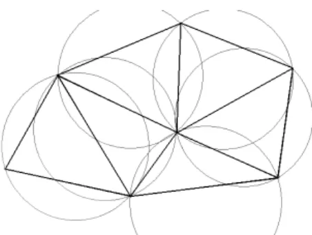
2.3.1 Delaunay Triangulation . . . 24

2.3.2 Delaunay Tetrahedralization . . . 25

2.3.3 Surface Mesh Generation . . . 27

(22)

2.3.3.1 Sphere Discretization . . . 28

2.3.3.2 Swept Primitives Discretization . . . 29

2.3.3.3 Surface Reconstruction . . . 29

2.4 Mesh Quality Measures . . . 31

2.4.1 Triangular Elements . . . 36

2.4.1.1 The Minimum/Maximum Angle . . . 36

2.4.1.2 The Aspect Ratio . . . 36

2.4.1.3 The Distortion Metrics . . . 36

2.4.2 Tetrahedral Elements . . . 36

2.4.2.1 Radius-edge ratio . . . 37

2.4.2.2 Aspect ratio . . . 38

2.4.2.3 Dihedral Angle . . . 38

2.5 Surfaces . . . 38

2.5.1 Surface Representation . . . 39

2.5.2 Bezier Surface . . . 42

2.5.3 B-Spline Surface . . . 44

2.6 Smooth Approximation of a Points Cloud . . . 46

2.7 Discussion . . . 49

3 Surface Mesh Post-Processing Methods 51

3.1 Smoothing Methods . . . 52

3.1.1 Averaging Methods . . . 53

3.1.2 Optimization-Based Methods . . . 53

3.1.3 Physically-Based Methods . . . 54

3.2 Clean-up Methods . . . 54

3.2.1 Shape Improvement . . . 54

3.2.2 Topological Improvement . . . 55

3.3 Refinement Methods . . . 55

3.3.1 Edge Bisection . . . 55

3.3.2 Point Insertion . . . 56

3.4 Local Mesh Modification Operators . . . 56

3.5 Hybrid Methods . . . 58

(23)

3.5.1.1 Geometric Surface Mesh . . . 60

3.5.1.2 The Geometric Support . . . 61

3.5.1.3 Unit Surface Mesh Construction . . . 62

3.5.2 Surazhsky and Gotsman’s Method . . . 63

3.5.2.1 Geometric Background . . . 64

3.5.2.2 Remeshing . . . 65

4 Remeshing Driven by Smooth Approximation of Model Surface 69

4.1 Avoiding the Planar Facets Triangulation . . . 71

4.2 Remeshing . . . 73

4.2.1 Approximation of the Model Surface . . . 75

4.2.2 Algorithm . . . 77

4.3 Implementation Characteristics . . . 80

5 Results 85

5.1 Models Generated by Boolean and Assembly Operations . . . 85

5.1.1 Results when the planar facet triangulation is avoided . . . 85

5.1.2 Results Applying the New Remeshing Scheme . . . 89

5.1.3 Discussion . . . 98

5.2 Models Generated by Acquisition Process . . . 100

6 Conclusions 115

6.1 Summary of the Accomplished Work . . . 120

6.2 Future Work . . . 123

Bibliography 124

(24)

✶

Introduction

Numerical methods based on spatial discretizations, as the finite element method, the

boundary element method, the finite volume method, and others, play an important role

in computer aided design (CAD), engineering (CAE), and manufacturing (CAM). Namely,

the finite element method (FEM) is probably the most widespread analysis technique in

the engineering community. This technique is capable of solving field problems governed

by partial differential equations for very complex geometries. However, successful and

efficient use of FEM still requires significant expertise, time, and cost.

Many researchers are investigating ways to automate FEM, thus allowing improved

productivity, more accurate solutions, and use by less trained personnel. Often the most

time consuming and experience requiring task faced by an analyst is the discretization

of the general geometric definition of a problem into a valid and well conditioned finite

element mesh. For complex geometries, the time spent on geometry description and mesh

generation are the pacing items in the computational simulation cycle. A particularly

complex example given by Mavriplis [Mav00] showed the mesh preparation time to be 45

times that required to compute the solution.

Automatic generation of consistent, reproducible, high quality meshes without user

intervention makes the power of the finite element analysis accessible to those not expert in

the mesh generation area. Therefore, tools for an automated and efficient mesh generation

(25)

are important prerequisites for the complete integration of the FEM with design processes

in CAD, CAE, and CAM systems.

Most of the research on development of fully automatic unstructured mesh generators

has been concentrated on various triangulation schemes. The advantage of them lies in

the fact that simplicial elements (triangles and tetrahedra) are most suitable to discretize

domains of arbitrary complexity, particularly when locally graded meshes are needed.

Over the past decades, a wide class of algorithms for the generation of triangular and

tetrahedral meshes has been established from three basic strategies: tree based approach,

advancing front technique, and Delaunay triangulation. While the meshing schemes for

the discretization of 2D problems matured into very robust and efficient algorithms, there

are still many open issues in 3D, including not only theoretical guarantee of convergence,

quality bounds but also implementation aspects as robustness and versatility.

The long-term goal for developers of meshing tools is the generation of high quality

meshes directly from CAD models, without user interaction.

1.1 Motivation

The finite element method is a powerful tool for the engineering community. One

of the barriers to automating finite element analysis is the automatic generation of high

quality meshes.

Triangle meshes are flexible and commonly used as boundary representation for

sur-faces with complex geometric shapes. In addition to their geometric qualities or

topo-logical simplicity, intrinsic qualities such as shape of triangles, their distribution on the

surface and the connectivity are essential for many algorithms working on them.

The quality of the volumetric mesh generated from the surface triangulation is directly

affected by the quality of the surface mesh. If the surface mesh quality is poor, the

volumetric mesh either cannot be generated or a poor quality volumetric mesh results.

In finite element analysis, the quality of the model surface approximation and the

mesh quality are very important. For example, if the elements angles become too large,

the discretization error in the finite element solution is increased and, if the angles become

(26)

regular meshes are necessary for engineers to perform effective finite element analysis.

The accuracy and cost of the analysis directly depends on the size, shape, and number of

elements in the mesh.

Unfortunately, most of surface meshes can hardly be called satisfactory without any

kind of post-processing to improve their intrinsic qualities.

In this context, improving the surface mesh quality is an almost obligatory step for

the mesh data in finite element analysis. This step must reduce or eliminate sharp angles,

improve the nodes distribution and their interconnections, while preserving the geometric

characteristics as much as possible.

1.2 The Problem Origin

Usually, automatic mesh generators can produce surface meshes with a specified

qual-ity degree for simple predefined primitives, like spheres, cylinders or prisms. However, to

generate models with high complexity two options frequently can be chosen: the

appli-cation of the Boolean (union, intersection or subtraction) and assembly operations over

predefined primitives; or the reconstruction of surfaces by an acquisition process, such as

medical imagery, laser range scanners, contact probe digitizers, radar and seismic surveys.

Unfortunately, both methods produce surface meshes with a large number of badly shaped

elements. For the Boolean and assembly operations, the elements in the intersection

ar-eas are usually split into degenerate ones, decrar-easing drastically the elements quality, as

Figure 1.1 illustrates. Each triangle from one object can be intersected by more than one

triangle in the other object, and this generates small and badly shaped triangles which

compose the resultant mesh. The surface meshes with this level of quality cannot be used

as input for finite element volumetric mesh generators.

Badly shaped triangles also raises in meshes generated by an acquisition process.

During the reconstruction process, the algorithm guarantees good approximation for the

geometry and topology, but it does not guarantee the triangle shape quality. In many

cases, the generated mesh possess a large amount of triangles and many of them are badly

shaped, which sometimes makes impracticable the volumetric mesh generation. Figure

(27)

(a) Gear Model (b) Three-phase transformer model

Figure 1.1: Examples of surface meshes generated by the application of Boolean and assembly operations over predefined primitives

(a) (b)

Figure 1.2: a) Reconstructed surface from a points cloud, b) zoom of a small part of the surface, [Goi04]

As consequence, the surface meshes of models generated by: the application of the

Boolean and assembly applications over simple models; or from an acquisition process,

should be improved, before being used as input to electromagnetic simulation by finite

element method.

1.3 Approach

The final goal of our project is the generation of high quality surface meshes for models

obtained by acquisition process or models resultants from the application of the Boolean

(28)

well conditioned finite element system that minimizes numerical errors and singularities

that might otherwise arise.

To improve the surface mesh quality, different post-processing methods can be used,

such as surface smoothing, cleaning-up, refining, adaptive methods, among others. This

work presents some advantages of using the mesh adaptation process to improve the mesh

quality. It works directly on the surface mesh and applies series of local modifications

operators on the mesh. These operators can enrich, simplify or improve locally the mesh.

To avoid losing model geometric characteristics, it is necessary to know the model surface

geometry.

Unfortunately, most of the time, only the mesh configuration is available. To overcome

this, it is important to have an approximation of the model surface geometry. We introduce

a smooth surface approximation evaluated by pieces from the mesh nodes to approximate

the model geometry. Each mesh face is approximated by a B-spline surface patch using

least squares formulation. The approximation is used to drive the nodes movements and

assure that they stay on top of the original model surface during the application of the

local mesh modifications.

The optimization procedure will then consist of analyzing the current mesh edges in

order to collapse the short edges, to split the large ones, to improve mesh connections and

distribution. Edge swapping and vertices relocations improve the elements shape quality.

The deviation between the mesh elements and the geometric approximation of the model

is controlled during the whole process.

1.4 Contributions

The main contribution of our work is the development of a remeshing method suitable

to improve indistinctly the surface mesh of models generated by application of Boolean

and assembly operation over 3D primitives and models reconstructed from a set of points.

It performs series of local mesh modifications driven by a smooth approximation of the

model surface.

We also introduce a new approach to evaluate the model surface approximation

(29)

generated by application of Boolean and assembly operation over 3D primitives and

mod-els reconstructed from a set of points.

1.5 Outline of this work

This document is organized in 6 chapters (including this one). Chapter 2 surveys

the general concepts of finite element method, geometric modeling, mesh generation and

mesh quality metrics. It also brings a brief study on surfaces and a technique to evaluate

a smooth surface approximation of a scattered set of points based on the least square

formulation.

In chapter 3, we discuss the state-of-the-art in surface mesh post-processing

meth-ods. The basic methods like smoothing, cleaning-up and refinement are presented first.

Following two remeshing techniques are detailed.

Chapter 4 presents our method to improve surface mesh quality, the remeshing driven

by smooth approximation of model surface. It preserves the geometric characteristics of

models that can be obtained after the application of the Boolean and assembly operations

to predefined primitives or reconstructed from a set of unorganized points.

In chapter 5, some results are shown to illustrate the accomplished work. The initial

mesh elements quality and the initial model geometry will be compared to the respective

results after the application of our remeshing approach.

(30)

✷

General Concepts

This project goal is to produce high quality meshes, to guarantee the evaluation of

accurate results in electromagnetic simulation throughout the finite element method.

In order to have a better understanding of the area where this work is inserted, this

chapter surveys the general concepts of finite element method, geometric modeling, mesh

generation, mesh quality metrics, surfaces and smooth approximation. The problems that

may arise during the mesh generation, surface reconstruction or after the Boolean and

assembly operations application are highlighted.

2.1 Finite Element Method

”The limitations of the human mind are such that it cannot grasp the behavior of its complex surroundings and creations in one operation. Thus the process of subdividing all systems into their individual components or ’elements’, whose behaviors is readily under-stood, and then rebuilding the original system for such components to study its behavior is a natural way which the engineer, the scientist, or even economist proceeds”- O. C. Zienkiewicz and R. L. Taylor (1989).

”Everybody nowadays knows what finite elements are: they are the methods for solving

(31)

boundary value problems in which one divides the domains of the problem into little pieces over which the solution is approximated using polynomials. The little pieces are finite elements, and the polynomials are called shape functions”- J. T. Oden (1990).

Many physical phenomena in science and engineering can be modeled by partial

dif-ferential equations (PDEs). When these equations have complicated boundary conditions,

are posed on irregularly shaped objects, or the domains include non-linear materials, the

PDEs usually do not admit closed-form solutions. A numerical approximation of the

solution is thus necessary.

The finite element method (FEM) is one of the numerical methods for solving PDEs. FEM evolved in the early 1950’s with the aim of solving mechanical engineering problems,

as heat diffusion, fluid flow, and stress analysis. In 1970, PP. Silvester and M. V. K Chari

proposed the use of this method for electromagnetic problems, including in its formulation

the solution of non-linear problems. The methods used before 1970 were not completely

satisfactory, in particular when the structure had a complex geometry or when nonlinearity

in ferromagnetic materials was considered [Ida97].

FEM numerically approximate the solution of a linear or nonlinear PDE by replacing

the continuous system with finite number of coupled linear or nonlinear algebraic

equa-tions. This process of discretization associates a variable to each node in the problem domain.

It is not enough to choose a set of points to act as nodes; the problem domain

must be partitioned into small pieces of simple shape. In the FEM, these pieces are called

elementsand they are usually triangles or quadrilaterals (in two dimensions) or tetrahedra or hexahedral bricks (in three dimensions). The FEM employs a node at every element

vertex; each node is typically shared among several elements. The collection of nodes

and elements is called a finite element mesh. Two and three-dimensional finite element meshes are illustrated in Figure 2.1.

Since the elements have simple shapes, it is easy to approximate the behavior of a

PDE on each element. The change of the dependent variable with regard to position

is approximated within each element by an interpolation function. The interpolation

function is defined relative to the values of the variable at the nodes associated with each

(32)

(a) Two dimensional mesh

(b) Three dimensional mesh

Figure 2.1: Finite element meshes

formulation. The interpolation functions are then substituted into the integral equation,

integrated, and combined with the results from all other elements in the solution domain.

The results of this procedure can be reformulated into a matrix equation of the form

AΦ =b , which is subsequently solved for the unknown variable.

The accuracy of the numerical solution depends on the size and also on the shape of

finite elements. The smaller are the elements, the closer the numerical solution will be

to the exact solution. But, as the number of elements increase, the processing time also

increases.

Considering the elements shape, various metrics of quality for first order triangular

and tetrahedral mesh elements have appeared in the mathematical and technical literature.

Some of these metrics are discussed in section 2.4.

Before the discretization of the problem domain into the finite element mesh, the

domain need to be modeled. Next section presents techniques to accomplish this.

2.2 Geometric Modeling

The term geometric modeling first came into use in the early 1970s with the rapidly

developing computer graphics, computer-aided design (CAD) and manufacturing (CAM)

technologies. It refers to a collection of methods used to define the shape and other

geometric characteristics of an object [Mor85].

When a model of something is constructed, it means to create a substitute of that

thing - a representation. If the model is a good one, it will respond to questions in the

(33)

for an objective, while ignoring other information. For many applications, the geometric

model of a physical object may require the complete description of surface reflectance

properties, texture and color; or it may include only information on elastic properties of

the object material. The required detail can be determined by the uses and operations

to which the model is intended to. If the model is rich enough in descriptive detail, one

can perform operations on it that yield the same results as operations performed on the

subject itself.

Geometric modeling methods are used to construct precise mathematical description

of the shape of a real object or to simulate some process. The geometric modeling is

divided in many subareas, among them three are the most common:

• Wireframe modeling: It describes the object in terms of its vertices and edges, the faces and other characteristics are referenced. It is simple to construct, but the

representation is usually ambiguous with lack of visual coherence and information

to determine the object interpretation;

• Surface modeling: It provides mathematical description of the shape of the objects surfaces, it also offers few integrity checking features. But surfaces are not

necessar-ily properly connected and there is no explicit connectivity information stored. This

subarea is often used where only the visual display is required, e.g. flight simulators.

• Solid Modeling: It contains information about the closure and connectivity of the volumes of solid shapes, it also guarantees consistent description of closed and

bounded objects and provides a complete description of an object modeled as a rigid

body in 3D space. Solid models enable a modeling system to distinguish between

the inside and outside of a volume;

Solid modelers permit rapid construction of finite element models. They associate the

geometric entities (abstract solids) to symbolic representations, throughout representation

schemes. The major representation schemes are the constructive solid geometry, the sweep

representation and the boundary representation. Following, these schemes are described

and their description is based on [Req80, Mag00a, Nun02] works. The schemes can be

used by themselves or combined forming hybrid representation schemes. The Boolean

(34)

of solid manipulation and, unfortunately, most of the time, the meshes quality degrades

after their application.

2.2.1 Constructive Solid Modeler

In constructive solid geometry (CSG) a solid is defined as a combination of simple

regular solids. This simple solids are called primitives, typically spheres, blocks,

cylin-ders, pyramids, torus, etc. The primitives are combined among themselves by a set of

Boolean and assembly operations or modified by geometric transformations to produce

more complex solids. The Boolean operations are the intersection, union and difference.

These operations are discussed in section 2.2.4.

Modeling a solid with this scheme is very intuitive for most users. The CSG models

are usually represented by CSG trees. Figure 2.2 shows the construction steps of a CSG

model.

(35)

2.2.2 Sweep Representation

The basic notion embodied in sweeping schemes is very simple: A solid is represented

by amoving object plus thetrajectory. The most common are the rotational and transla-tional sweep of 2D primitives (circles, squares, rectangles, etc. ), Figure 2.3 presents both

of them.

(a) Rotational (b) Translational

Figure 2.3: Sweep Solids [Mag00a]

Usually, this scheme is used to represent the primitives of the CSG models.

2.2.3 Boundary Representation

A boundary representation (B-rep) represents a solid by segmenting its boundary into

a finite number of bounded subsets. Each B-rep element of the model is formed by a set

of other elements, following a hierarchy: the model is formed by a set of regions, that are

formed by a set of shells, that are formed by a set of faces that posses edges delimited by

vertices, which represents the minimum structure, as shown in Figure 2.4.

(a) Region (b) Faces (c) Edges and

Vertices

Figure 2.4: B-rep elements [Mag00a]

(36)

Mag00b]. It implements the use concept, which enables the multiple existence of the basic topological elements (vertex, edge or face) to share the same geometry and form.

For example, any internal face of the model make reference to exactly two FaceUses and all model boundary faces make reference to only oneFaceUse (the one that takes part in the model). Theuse concept can also be applied to vertices and edges and these elements can have two or more uses. This concept is illustrated in Figure 2.5.

Figure 2.5: Main features of B-rep structure [Mag00a, Nun02]

Each bounded region has its own orientation (direction), compatible with the

orien-tation of the other components. Each FaceUses is oriented by the outer LoopUse. The Holes on the face are defined by counter-oriented loops. Each LoopUse is composed of a sequence ofHalfEdges related toEdgeUses, which are finally bounded by twoVertexUses. The HalfEdges are responsible for the model orientation and they are always treated in pairs (called mates) belonging to the same region. Figure 2.6 shows how the B-rep elements interact. The structure is represented in UMLi

notation.

The B-rep data structure (Figure 2.6), involves the primitive elements Model, Region, Shell, Face, Edge, HalfEdge and Vertex. Face, Edge and Vertex have derivative elements representing their occurrence in each region (FaceUse,EdgeUse andVertexUse) and their geometry (FaceGeom,EdgeGeom andVertexGeom). Faces do not have any direction, but FaceUses do. So, the loop concept is related to theFaceUse direction, and is, then, called LoopUse. Auxiliary structures link all the uses of one edge to the uses of edges in one shell. The same situation occurs between the uses of one vertex and the uses of vertexes

in one shell. All the topological structure are based on double linked lists. In these lists,

only the head node makes reference to the element that is hierarchically one level higher. i

(37)

Figure 2.6: B-rep data structure [Nun02]

Usually, the B-rep models are built by a sequence of Euler operators to guarantee valid

solids constructions. Next section presents a brief explanation about these operators.

2.2.3.1 Euler Operators

A B-rep solid is considered topologically correct if its elements are well connected

(ex: faces are bounded by edges which, then, connect two vertexes). The assurance

of topological validity is obtained by Euler operators [Mag00a, Mag00b, Nun02]. To

guarantee the solid topological validity, a variation of Euler formula was defined:

V ₋E+F ₋L= 2_∗(R+S₋H) (2.1)

being V, E and F, respectively, the number of vertex, edges and faces; L is the number

(38)

shells (holes in regions) and it is the component genus (which corresponds toH, ofHole).

The Euler operators defined to the presented B-rep data structure are presented on

Table 2.1. Even though the nomenclature and description use the words Face, Loop,

Edge and Vertex, the operators will be applied to the use of these elements. The word

use was omitted to facilitate the association between the elements and letters used in the name of the operators. For example, the operator MVFR introduces a new region to the

B-rep model. The new region starts with one vertex and one face. The operator MEV

introduces a new vertex and a new edge to the data structure. The new edge is connected

from an existent vertex to the new one.

Table 2.1: Basic Euler operators defined to the B-rep data structure [Mag00b] Operator Description

MVFR Make Vertex, Face, Region KVFR Kill Vertex, Face, Region

MEV Make Edge, Vertex KEV Kill Edge, Vertex MEF Make Edge, Face KEF Kill Edge, Face MEKL Make Edge, Kill Loop KEML Kill Edge, Make Loop MFKLH Make Face, Kill Loop Hole KFMLH Kill Face, Make Loop Hole

MSKR Make Shell, Kill Region KSMR Kill Shell, Make Region MFFR Make double Face, Region KFFR Kill double Face, Region

2.2.4 Boolean and Assembly Operations

The Boolean operations allow users to perform operations like union, subtraction and

intersection over simple models to generate new models with higher complexity.

Assemblies are very important in electromagnetic problems where objects are

com-posed of parts with different materials in direct contact. When the FEM is used to solve

these problems, it is necessary to interpret the common boundary between the parts as a

single piece, even when the parts are used separately to perform other operations. Doing

(39)

for instance, the air that involves an electrical device. This air region can be easily shaped

using the assembly operation performed in a box assembled to an electrical device located

in its interior. A model for an assembly should reflect its important geometric properties:

the shape, the arrangement and the individual characteristic of its components [Arb90].

The algorithm to generate the polygonal representation is called boundary evaluator. The process of boundary evaluation presented here is based on works [Nun03, Mag00a].

This process follows thedivide and conquer algorithm presented in [Req85, Til80]. It has four steps:

1. mesh generation over primitives;

2. intersecting process;

3. elements classification;

4. Boolean evaluation and elimination of all undesired elements.

Each step returns a consistent and compatible polygonal mesh to be used in the

next step, until the result is achieved. Compatible polygonal mesh means that there is

coincidence among vertex and edges endpoints. Figure 2.7 shows examples of a compatible

mesh and a non compatible one.

(a) Compatible mesh ex-ample

(b) Non-compatible mesh example

Figure 2.7: Examples of compatible and non-compatible meshes

The three first steps of the boundary evaluation are common to all operations. Only

the Boolean evaluation and the elimination of undesired elements are specifically done,

according to the executed operation.

Before starting this work, a triangular representation of a model was a prerequisite

(40)

them is easier than working with polygonal meshes. The following subsections explains the

boundary evaluation steps for general polygonal meshes and how it affects the resultant

mesh quality.

2.2.4.1 Primitive Mesh Generation

The first step of boundary evaluation is the generation of surface mesh over

primi-tives. Many solids in engineering problems have curved surfaces. These solids can not be

represented by a collection of polygons without precision losses: the polygonal

represen-tation is only an approximation of the real solid. However, the polygonal mesh is very

flexible and can be automatically generated.

The 3D primitive can be chosen from a set of predefined ones (ellipsoids, torus,

cylin-ders or prisms), swept primitives, which are generated by applying sweep operations

(translational or rotational) to 2D primitives (arcs or polylines) or it can be a

recon-structed surface. Methods to generate surface meshes for these 3D primitives are detailed

in section 2.3.3.

2.2.4.2 Intersecting Process

Finding the intersection points is the first step in the intersecting process. In order

to accomplish this, the convex hull of each object is tested. If intersections exist, all

components of one object need to be compared in relation to the other object components,

to identify the intersection points. After evaluating all the intersection points and edges,

they are separated into two groups: i) points located on facet’s boundary and ii) points

and edges located inside the facets. The first group is directly inserted into the data

structure. Then each facet and the second group are triangulated using a constrained 2D

Delaunay mesh generator [She96]. The data structure modifications are realized by the

application of the Euler Operators 2.2.3.1.

The evaluation of the intersection points between triangular surface meshes is easier

than in polygonal surface meshes. There are a limited number of possible combinations

between triangles, as Figure 2.8 illustrates.

(41)

compati-Figure 2.8: Possible combinations between triangles [Mag00a]

ble, correct and formed by triangular faces. It will be ready for the elements classification.

The elements quality deterioration that may appear in the resultant mesh occurs in

this step. Each element from one object is commonly intersected by more than one element

from other object, as in Figure 2.9(a). The small and badly shaped triangles appear when

the triangulation is regenerated, as shown at Figure 2.9(b). The new triangles form the

resulting mesh.

(a) Before (b) After

Figure 2.9: The shaded part represent the triangles generated after the intersections are evaluated

2.2.4.3 Elements Classification

When all intersections have been computed, each element of one shell needs to be

(42)

shared oron anti-shared, depending on the orientation. This step is executed twice, once for the shell Aelements and another for shell B elements.

Vertex is the first one to be classified. The raycasting technique is applied to classify a vertex from shellA, when it is noton a shell B. This technique is shown in Figure 2.10.

Figure 2.10: Raycasting technique

Inraycasting, an arbitrary ray passing by a vertex of shellAis chosen and the number of intersections of this ray in shell B is evaluated. If it is even, the point is classified as out, and if it is odd, the point receives in as its classification.

When the vertex classification is over, the edges classification starts. This

classifica-tion is done applying Table 2.2. Whether one vertex is not on the other shell, the edge receives this vertex classification. For on/on endpoints classification, the edge mid point needs to be classified by raycasting and the edge receives its classification. If the inter-secting process was correctly executed the classification in/out can not exist. In Table 2.2, ”RAY” meansraycasting and ”ER”, error.

Table 2.2: Edges Classification [Arb90]

Endpoints OUT/OUT OUT/ON ON/ON IN/ON IN/IN OUT/IN

Edges OUT OUT RAY IN IN ER

The loops are classified according to their edges classification. A loop with one vertex

has its classification. Whether one loop edge is noton the other shell the loop receives its classification. If a loop has edges with in and out classification that means error in the intersecting process. When all loop edges areon, the loop ison and an equal loop exists in the other shell. The orientation of these loops are compared and the loop receives an extra

classification: shared for the same orientation and anti-shared for opposite orientation. To finish, the face will receive the extern loop classification. All possible combinations for

(43)

Table 2.3: Faces Classification [Arb90]

Edge OUT OUT OUT OUT OUT OUT OUT OUT OUT

Edge OUT OUT OUT IN IN IN ON ON ON

Edge OUT ON ON OUT IN ON OUT IN ON

Face OUT ER OUT ER ER ER OUT ER OUT

Edge IN IN IN IN IN IN IN IN IN

Edge OUT IN ON OUT IN ON OUT IN ON

Face ER ER ER ER IN IN ER IN IN

Edge ON ON ON ON ON ON ON ON ON

Edge OUT IN ON OUT IN ON OUT IN ON

Face OUT ER OUT ER IN IN OUT IN ON

2.2.4.4 Boolean Evaluation and Elimination of Undesired Elements

The previous steps are common for all Boolean and assembly operations. Now, each

operation has a different treatment.

Boolean evaluation consists in deciding which elements remains and which will be

eliminated. Each face received one of the eight possible classification. The A elements

are: onAinB, onAonBshared, onAonBanti-shared or onAoutB, while the B elements are: onBinA, onBonAshared, onBonAanti-shared or onBoutA. For each classification and op-eration, an action is performed, Table 2.4 shows the necessary action for each face

clas-sification. In this table, A+B corresponds to the assembly operation and ”A-Shared”

meansanti-shared. The Euler operators are used to update the B-rep data.

Table 2.4: Decision Table for Boolean and Assembly Operations [Muu91]

A B A−B A∪B A∩B A+B

ON IN kill kill retain retain ON ON SHARED kill retain retain retain ON ON A-SHARED retain kill kill retain ON OUT retain retain kill retain IN ON retain+flip kill retain retain ON SHARED ON kill kill kill kill ON A-SHARED ON kill kill kill kill OUT ON kill retain kill retain

After implementing all Boolean evaluation steps, a correct triangular mesh is achieved.

This mesh may be used as the input to another operation or to the volumetric mesh

(44)

2.3 Finite Element Mesh

As defined in the section 2.1, a finite element mesh is a discretization of a geometric

domain into small simple shapes. Discretizing an object is a more difficult problem than

it appears at first glance. A useful mesh should satisfy constraints that sometimes seem

almost contradictory. A mesh must conform the object and ideally should meet constraints

on size and shape of its elements.

Consider first the goal of correctly modeling the shape of a solid. Scientists and

engi-neers often wish to model objects with complex shapes and possibly with curved surfaces.

Boundaries may appear in the interior of a region as well as on its exterior surfaces. They

are typically used to separate regions that have different physical properties. In practice,

curved boundaries can often be approximated by piecewise planar boundaries, so

theoret-ical mesh generation algorithms are often based upon the idealized assumption that the

input geometry is piecewise linear. Given an arbitrary straight-line two dimensional

re-gion, it is not difficult to generate a triangulation that conforms to the shape of the region.

But, finding a tetrahedralization that conforms to an arbitrary linear three-dimensional

region is trickier [She97].

Another goal of mesh generation is that the elements should be relatively well shaped.

Elements with small angles may degrade the quality of the numerical solution, because

they can make the system of algebraic equations ill-conditioned. Whether a system of

equations is ill-conditioned, roundoff error degrades the accuracy of the solution if the

system is solved by direct methods, and the convergence is slow if the system is solved by

iterative methods. By placing a lower bound on the smallest angle of a triangulation, one

is also bounding the largest angle; for instance, in two dimensions, if no angle is smaller

than θ, then no angle is larger than 180₋2θ. Hence, many mesh generation algorithms

take the approach of attempting to bound the smallest angle.

Satisfying both constraints of element size and shape are difficult, because the

ele-ments must meet only at their vertices. The edge of one triangular element can not be a

portion of an edge of an adjoining element and also a face can not be a portion of other face

as Figure 2.11 illustrates. There are variants of methods like the finite element method

that permit such noncompatible elements. However, such elements are not preferred, as