Paulo Roberto M. Lyra
Member, ABCM [email protected] Federal University of Pernambuco – UFPE Departamento de Engenharia Mecânica 50740-530 Recife, PE. BrazilDarlan Karlo E. de Carvalho
[email protected] Federal University of Pernambuco – UFPE Departamento de Engenharia Civil 50740-530 Recife, PE. BrazilA Computational Methodology for
Automatic Two-Dimensional
Anisotropic Mesh Generation and
Adaptation
This paper describes a versatile computational program for automatic two-dimensional mesh generation and remeshing adaptation of triangular, quadrilateral and mixed meshes. The system is flexible to be incorporated into an adaptive global or local remeshing procedure and for generating both, iso and anisotropic meshes. The main contribution of this work is to extend well established procedures for the generation and adaptation of both, iso and anisotropic triangular meshes, such as local and global remeshing as well as boundary layer mesh generation, to deal with iso and anisotropic quadrilateral and mixed meshes. Several examples are presented to illustrate the quality of the meshes produced, and the flexibilities of the computational system.
Keywords: Iso and anisotropic mesh generation, adaptive remeshing, triangular,
quadrilateral and mixed unstructured meshes
Introduction
1
The use of an adequate mesh consists in one of the main ingredients for an accurate numerical simulation. In order to obtain such a mesh, a versatile mesh generator and a mesh adaptive procedure must be available. Automatic mesh generation has received much attention from researchers on computational simulation, to minimize manual intervention, to improve mesh quality and to obtain more efficient procedures. Unstructured methodologies are becoming predominant due to the ability of modeling geometrically complex designs and because they are the natural environment for adaptivity, which may be the only hope for resolving very small scale features (e.g. boundary layers). Most finite element and finite volume codes use unstructured triangulations due to their geometrical flexibility and the low cost of linear triangular elements. However, certain formulations perform better with quadrilateral elements and it may be necessary to use different types of elements for different physics when solving coupled problems. In fluid-structure interaction problems, for instance, it is very common to use unstructured triangular meshes for the fluid and quadrilateral meshes for the structural problem. In computational fluid dynamics applications, it may also be interesting to use a mixed mesh, in which quadrilateral elements are used in regions where the flow is essentially one dimensional (Hwang and Wu, 1992). The utilization of unstructured mesh generation techniques for the simulation of boundary layer problems (Hassan, 1994, Marcum, 1995 and Thompson et al., 1999), (e.g. viscous flow) and for anisotropic adaptation is of great importance (Peraire et al., 1987, George, 1991, Borouchaki and Frey, 1998, Thompson et al., 1999 and Almeida et al., 2000) since the obtained meshes are capable of improving the accuracy of the numerical solution while at the same time improving the efficiency of the numerical method, as they guarantee an “optimal” number of elements in the mesh. The development of procedures for the generation of anisotropic unstructured meshes of triangles capable of capturing directional features of the physical problem is a topic of intensive research (Jansen and Shephard, 2001), but less work has been done regarding anisotropic meshes of quadrilaterals (Borouchaki and Frey, 1998). Some effort has also been made in order to build unstructured hexahedral meshes. However, most of the success achieved concentrates on generating quadrilaterals and
Paper accepted June, 2006. Technical Editor: Aristeu da Silveira Neto.
hexahedra in the vicinity of solids walls, i.e. inside boundary layers. It is known that quadrilateral and hexahedra require less cpu time and memory whenever an edge-based data structure is adopted for both finite element (FEM) and finite volume methods (FVM), (Borouchaki and Frey, 1998). Apart from that, it also improves accuracy in the FVM context (Hwang and Wu, 1992 and Borouchaki and Frey, 1998). However, the FEM does not always share the last property (Lyra and Almeida, 2002). Building good quality quadrilateral and mixed meshes is very challenging because quadrilaterals are very “stiff'' from a geometric point of view, and controlling element distortion in complex domains during analysis that incorporate adaptive procedures is certainly not an easy task.
In this work, an automatic triangular mesh generator based on the advancing front technique (Peraire et al., 1987) is used as the main building block of a computational system for mesh generation that can build triangular, quadrilateral and mixed meshes over arbitrary domains. Quadrilateral elements are generated from an original mesh of triangles through a process of merging and splitting. These approaches allow a good control of the mesh density and gradation, and of the directional stretching and quality of both, triangular and quadrilateral elements. The so called “advancing layers'' technique (Hassan et al., 1994), which was originally devised to generate triangular/tetrahedral meshes, is also extended to deal with quadrilateral and mixed meshes allowing the construction of adequate meshes within the regions close to solid boundaries. The system also allows for either, a global adaptive remeshing procedure (Peraire et al., 1987), in which the whole mesh is re-built according to the mesh parameters dictated by the error estimate, or a local remeshing (Hassan et al., 1993a), in which we determine automatically the subregions within the domain where the mesh must be re-built.
meshes and the importance of using a flexible and robust mesh generation/adaptation procedure when dealing with complex geometries and/or problems which involve complex features.
Unstructured 2-D Mesh Generation
The mesh generation problem consists in subdividing an arbitrary domain into a consistent assembly of elements (subregions). If the generated elements cover the entire domain and the intersection of the elements occurs only on common points or edges, the consistency of the mesh is guaranteed. According to Peraire (1987), the basic requirements for a mesh generator are:
a. Capacity to handle arbitrary geometries with minimum user
intervention;
b. The necessity of as little input data as possible;
c. Good control over the spatial variation of size and shape of the elements.
d. Easy incorporation of adaptive strategies.
Triangles are the most flexible elements for automatic mesh generation over complex two dimensional geometries, particularly when mesh grading is required. Several robust and versatile unstructured triangular mesh generators and their extensions for 3-D geometries (tetrahedral mesh generators) have been developed and are currently used in academic and industrial environments. There are several well-established triangulation procedures, such as the advancing front (Peraire et al., 1987 and Thompson et al., 1999) and the Delaunay triangulation (Schroeder and Shephard, 1990, Thompson et al., 1999, and Secchi and Simoni, 2003).
Advancing Front Triangular Mesh Generator
The original advancing front algorithm has been developed over time into a family of programs which are very reliable and flexible for an easy incorporation of mesh adaptation. The advancing front mesh generator can be described as in Algorithm 1.
Algorithm 1. Advancing front technique.
1. Input of geometric data (using control points); 2. Input of mesh control parameters (through a
background mesh);
3. Geometric modeling (using cubic splines); 4. Boundary discretization (placing new points on
the boundary);
5. Domain discretization (simultaneously generating points and triangles);
6. Mesh quality enhancement (through topological and geometrical strategies).
The computational domain is modeled through the use of cubic splines which are defined by some control points. Close to singularities extra care must be taken in the definition of these points in order to avoid failure (Thompson et al., 1999).
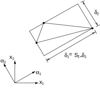
As a “pre-processing” stage, before the mesh generation begins, we must first build an initial and very coarse triangular background mesh that covers the whole domain. This coarser mesh is used only to provide a piecewise linear spatial distribution of the nodal parameters over the mesh to be constructed. Typically, elements of the generated mesh will have a projected length of δ2 in the direction parallel to α2 and a projected length of Stδ2 in the
direction normal to α2 (see Fig. 1), with St being the stretching
factor. During the generation process, the local values of these parameters will be obtained by a linear interpolation over the
δ
1= S
t
δ
2δ
2α
α
x
1 2
1
.
x
2Figure 1. Mesh parameters.
The boundary of the domain is represented by the union of boundary segments forming closed loops. External boundaries are defined in an anti-clockwise fashion while inner boundaries are set in a clockwise manner. As described previously, the generation of a triangular mesh by the advancing front technique begins by the discretization of the boundary of the domain. New points are created according to the mesh parameters which are interpolated from those of the background mesh. At the beginning of the process, the generation front is made by a set of linear segments connecting the boundary nodes. With the initial front defined, one segment is chosen and, in general, a triangle is created through the insertion of an internal node or by simply connecting existing nodes. New triangles are built following the same procedure. During the process any segment available to build a new triangle is set as “active” and the others which are set as “non-active” are removed from the generation front. Therefore the boundary segments are not modified during the mesh generation. The procedure continues until the whole domain is discretized. When solving problems which develop some essentially one dimensional features at certain regions (e.g. boundary layer, shocks, etc.) it is not very efficient to use uniform isotropic meshes. In these cases, it is important to have the possibility to define a direction and a stretching factor for the elements close to such regions. At least for linear triangular elements, the use of anisotropic meshes can be extremely important in terms of computational effort and accuracy (Rippa, 1992). To generate an anisotropic triangulation of the desired domain, it is used a transformation T which is a function of the mesh parameters, i.e. αi and δi, i = 1, 2. This transformation (see Peiró et al., 1994), is given by,
(
)
(
)
1 1 ,
=
=
∑
N ⊗i i i i
i i
T α δ α α
δ (1)
provides an accurate geometric modeling and high quality meshes, where the high level of control of the distribution of local mesh parameters eases the incorporation of mesh adaptation strategies. The quality of the meshes is strongly influenced by the mesh optimization stage. A specific mesh improvement strategy for highly anisotropic meshes and the definition of an adequate sequence of mesh enhancement procedures are incorporated into the code. Several other modifications have been introduced in the original code in order to incorporate the flexibility to deal with predefined multidomains and automatically defined subregions, to build boundary layer meshes, to make possible generating quadrilateral and mixed meshes and the automatic definition of which domains or subregions should be filled up by triangular or by quadrilateral elements. These features will be fully described in the correspondent sections.
Quadrilateral Mesh Generator
Unstructured quadrilateral meshes can be automatically generated in several different ways and do not impose serious topological restrictions on the meshes, being appropriated to deal with complex geometries, naturally allowing local non-uniform mesh refinement. Several different approaches have been proposed to generate unstructured quadrilateral meshes. These methodologies can be divided into two basic groups: those that try to generate quadrilaterals directly (Blacker and Stevenson, 1991, Zhu et al., 1991, Sarrate et al., 1993 and Gendong and Li, 1996), and those that convert a previously generated mesh of triangles into a mesh of quadrilaterals (Lee and Lo, 1994, Xie and Ramaekers, 1994, Alquati and Groehs, 1995, Lyra et al., 1998 and Lee et al., 2003). The conversion of triangular meshes is particularly attractive because these meshes can inherit the properties of the triangular meshes, whose generators are very well developed and once it is always possible to build a triangular mesh over any arbitrary 2-D domain, quadrilateral meshes can be constructed as general as the triangular ones. It also allows the use of any triangular mesh generator as a “black box”, even commercial ones for which source codes are not available, including procedures such as Delaunay methods (Weatherill, 1990) modified quadtree techniques (Schroeder and Shephard, 1990), etc. In the work of Ait-Ali-Yahia et al. (1996), anisotropic unstructured quadrilateral meshes were built using an edge-based error estimate and mesh movement. In the work of Borouchaki and Frey (1998), anisotropic quadrilateral meshes are generated using a more general approach based on defining an anisotropic discrete metric mapping. However, apart from the mentioned references, very little have been done with respect to anisotropic fully unstructured quadrilateral meshes. Here, the use of simple strategies during the conversion and mesh quality enhancement steps allows us to get reasonably good anisotropic quadrilateral meshes.
Indirect Approach: Conversion of Triangular Meshes
As we generate a quadrilateral mesh using the conversion strategy, the quadrilateral mesh inherits the characteristics of the initial triangulation. For both, iso and anisotropic meshes this strategy consists of four main steps, as presented in Algorithm 2.
Algorithm 2. Indirect approach for quadrilateral mesh generation.
1. Generate a triangular mesh (either iso or anisotropic);
2. Remove an edge between two adjacent triangles, to form
a quadrilateral;
3. Split all elements in the intermediate mixed mesh (triangles into three quadrilaterals and quadrilaterals into four quadrilaterals);
4. Perform some post processing steps in order to enhance mesh quality.
The standard strategy of merging triangles into quadrilaterals consists in eliminating a common edge that belongs to two adjacent triangles. Following the work done by Xie and Ramaekers (1994) and Alquati and Groehs (1995), our mesh generator is such that it refrains from merging triangles that would form a non-convex quadrilateral. Besides, for anisotropic meshes, the merging process will remove a common edge between two adjacent triangles, only if the two quadrilaterals to be created satisfy a quality criteria which is controlled by two geometric parameters, φ which is defined in Lee and Lo (1994), and the minimum internal angle θ. These parameters are compared to user defined tolerances φMIN and θMIN,
and if, for an inner edge, φ > φMIN and θ > θMIN this edge is
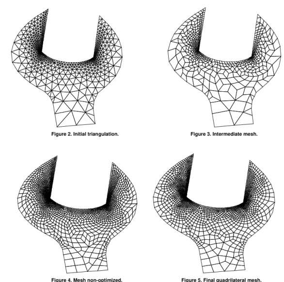
marked to be eliminated. We have attempted other strategies, in which the edges are previously grouped in some order (Alquati and Groehs, 1995), but our experiments have shown no significant improvement on the final mesh quality. Additionally, when dealing with anisotropic meshes, we redefine the merging procedure (step 2 of Algorithm 2), which is now performed as long as the common edge is one of the two biggest edges of both triangles and we also try to minimize the number of isolated triangles remaining after the merging step, by relaxing the quality criteria, as in general those isolated triangles will lead to bad quality quadrilaterals. The enhancement of the mesh quality (step 4) is slightly different for iso and anisotropic meshes and will be described later on this paper. The adopted procedure generates a quadrilateral mesh with edges that are approximately half of those of the corresponding triangular elements and usually this is not a serious concern, since the user can generate a coarser initial triangulation to obtain the desired mesh density. The four steps involved in the quadrilateral mesh generation can be seen in Figs. 2 to 5.
Multi-Domains and Mixed Meshes
method. In Algorithm 3 it is presented the strategy we have devised to create multi-domains and mixed meshes over predefined subdomains.
Figure 2. Initial triangulation. Figure 3. Intermediate mesh.
Figure 4. Mesh non-optimized. Figure 5. Final quadrilateral mesh.
Algorithm 3. Generation of multi-domains and mixed meshes.
1. Independent triangulation of each subdomain; 2. Predefinition of which subdomains will be filled up
with quadrilaterals;
3. Subdivision of triangles over triangular regions (splitting each triangle into four);
4. Conversion of triangles into quadrilaterals over the predefined regions (Algorithm 2);
5. Optimization of the created quadrilaterals.
The aforementioned mesh optimization process (step 5 in Algorithm 3) is only performed over quadrilaterals due to the fact that the new triangles are created in such a way that they inherit the quality of the “father” triangle, which was already optimized during the initial triangulation. The whole procedure can be illustrated through an academic example in the sequence of meshes shown in Figs. 6 to 9, where we have consistent assemblies of triangular and quadrilateral elements for complex geometries.
Figure 6. Initial triangular mesh.
Figure 7. Intermediate mesh.
Figure 8. Mesh non-optimized.
Figure 9. Final mixed mesh.
Figure 10. Directional mixed mesh without stretching. Figure 11. Directional mixed mesh with stretching.
Boundary Layer Unstructured Meshes
One alternative for the generation of meshes suitable for viscous flow simulations consists in the development of a mesh generator which generates a structured grid in the immediate vicinity of the solid surfaces and completes the triangulation using the unstructured mesh approach, leading to the so called hybrid meshes. This procedure has been successfully used for many realistic viscous flow simulations, see for instance Weatherill (1990). However, this approach is not very flexible for the inclusion of adaptivity or the extension for general complex 3-D configurations. Alternatively, the approach, presented by Hassan et al. (1991) and further developed in reference Hassan et al. (1993b), for generating and adapting fully unstructured viscous meshes, overcome the shortcomings mentioned above and presents as a good choice. This strategy is normally referred to as “advancing layers” and it basically consists in a modification of the usual advancing front technique in which a set of layers of stretched elements are created adjacent to the
Algorithm 4. Advancing layers algorithm.
1. Creation of the first layer of nodes and elements adjacent to solid walls through an advancing front procedure;
2. Movement of the non-boundary nodes towards the solid walls using a predefined distance and keeping the consistency of the mesh;
3. Elimination of non-desired elements;
4. Repetition of steps 2 and 3 through a continuous reference to a control function of the mesh or until a user defined number of layers is achieved;
5. Triangulation of the rest of the domain using the advancing front technique.
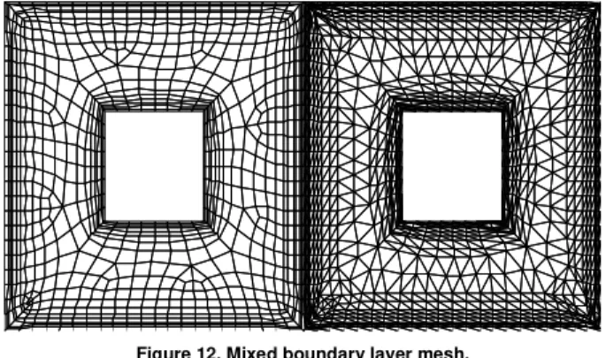
For further details see Hassan et al. (1991), and for other alternatives see for instance, Marcum (1995) and Thompson et al. (1999). As mentioned before we have extended this technique to deal with quadrilateral and mixed meshes. This feature can be extremely useful to handle boundary layer problems. By using the criterion proposed in this paper for merging anisotropic triangles into quadrilaterals, an important feature of our mesh generation procedure is that, even when tackling with multiple domains, the quadrilateral or mixed meshes generated keep the anisotropic feature of the initial triangular mesh near the boundaries. A key point to get good quality meshes, both inside and outside the boundary layer regions, is to prevent the Laplacian smooth for all nodes inside the boundary layer when dealing with quadrilateral meshes. The flexibility to deal with multi-domains mixed meshes incorporating boundary layer elements can be seen in Fig. 12 and a zoom on the boundary layer region is shown in Fig. 13.
Figure 12. Mixed boundary layer mesh.
Figure 13. Zoom of the mixed boundary layer mesh.
Some Important Numerical and Implementation Issues
Assessment of the Mesh Quality
For the triangular and quadrilateral elements quality assessment, we used, respectively, the ε and φ parameters (Lee and Lo, 1994). These metrics depend basically on the shape of the triangles and quadrilaterals. The ε parameter varies on the range [0,1], and for equilateral triangles ε=1. The φ parameter also varies between 0 and 1 for convex quadrilaterals, with φ=1 for rectangles. For non-convex quadrilaterals φ is negative. Apart from using the φ parameter, we can assess the quality of a quadrilateral element by the values of its internal angles. According to this criterion the shape of a quadrilateral is satisfactory if all of its angles satisfy the recommended range (Zhu et al, 1991) of 45o≥ ≥θ 135o. If an element do not satisfy the previous condition, Zhu et al. (1991) affirms that a quadrilateral element is not satisfactory if any of its
internal angles is out of the following acceptable
range 30o≥ ≥θ 150o. For both parameters, ε and φ, we can also define the geometric mean values εm and φm which are used to evaluate the quality of the triangular and quadrilateral meshes, respectively. For mixed meshes, we use the parameter ϕm, which is
the geometric mean of εm and φm. According to Lee and Lo (1994), an isotropic triangular mesh is of good quality when
m>0.87
ε and excellent if εm>0.94. If φm>0.54 the isotropic
quadrilateral mesh is considered good and if φm>0.72 the mesh is considered excellent. Mixed isotropic meshes, compounded of triangles and quadrilaterals, are considered extremely good if
m>0.69
ϕ . All these values of quality measurement are set rather arbitrarily for the purpose of comparison. Another criterion such as the number of elements connected to a node, which is ideally six for an internal node on triangular meshes and four on the quadrilateral ones, can be used as a measure of the quality of the meshes. The stretching ratio of a quadrilateral element, defined here as the ratio between the largest and the smallest distances between any two nodes of an element, is another quality parameter. We monitor these values to avoid excessively distorted elements on isotropic meshes.
It is worthy mentioning that different metrics have been proposed and can be used to assess the quality of both, triangular and quadrilateral isotropic meshes (Knupp, 2003 and Secchi and Simoni, 2003). For anisotropic meshes the quality of the mesh is extremely case dependent and, as far as the authors know, there are no simple parameters to assess the quality of those meshes. In such case we must relax on the requirements for the quadrilateral meshes to be acceptable and the final answer, whether the mesh is good or not, is given by the performance of the numerical analysis using such meshes.
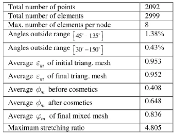
Table 1. Assessment parameters for mesh of Fig. 9.
Total number of points 2092
Total number of elements 2999
Max. number of elements per node 8 Angles outside range 45−135 1.38%
Angles outside range 30−150 0.43%
Average εm of initial triang. mesh 0.953
Average εm of final triang. mesh 0.952
Average φm before cosmetics 0.408
Average φm after cosmetics 0.648
Average ϕm of final mixed mesh 0.836
Maximum stretching ratio 4.805
Control and Improvement of Mesh Quality
In general, finite element analysis using triangular elements is less sensitive to element distortion than using quadrilateral or mixed meshes. For the latter, the control of the mesh quality, and therefore of the shape of the elements, is very important because the results of the analysis obtained using quadrilateral elements can be seriously compromised due to high element distortion (Bathe, 1996). Element distortion can have bad effects on the rate of convergence of finite element solutions and also introduces error when using numerical integration. The mesh generator should therefore be able to prevent excessively large aspect ratios and geometric distortion to keep the actual rate of convergence as close as possible to the theoretical one and the precision of the numerical integration. Finally, it is important to remark that mesh distortion problems are even more serious if higher order elements are attempted. In order to improve the quality of the mesh and to reduce the effect of the mesh distortion in the numerical solution, two mesh optimization sequences can be adopted. The choice of the sequence depends on whether the mesh is triangular or quadrilateral and whether it is iso or anisotropic.
Triangular Meshes
For triangular meshes the strategy adopted can be seen in Algorithm 5.
For both, iso and anisotropic meshes we have included an extra diagonal swapping (step 5 of Algorithm 5). For isotropic meshes the second diagonal swapping (step 5 of Algorithm 5) is also performed in order to obtain a more even distribution of the number of elements per node. Most of these procedures are standard and further details can be found in literature (Peraire et al., 1987, George, 1991, Peiró et al., 1994 and Thompson et al., 1999). For anisotropic meshes this second diagonal swapping can be extremely important in order to eliminate angles too obtuse. Considering Fig. 14, this swapping criterion can be summarized as described in Algorithm 6.
Algorithm 5. Mesh optimization sequence for triangular meshes.
1. Node elimination (remove nodes surrounded by three elements);
2. Laplacian smoothing (move nodes using an “elastic spring analogy”);
3. Diagonal swapping (try to get a more even number of triangles per node);
4. Laplacian smoothing (move nodes using an “elastic spring analogy”);
5. Diagonal swapping (iso and anisotropic meshes).
Algorithm 6. Diagonal swapping to eliminate highly obtuse angles.
1. Set Maxang = User predefined threshold;
2. Compute Maxbef = Maximum angle before
swapping;
3. Compute Maxaft = Maximum angle after swapping;
4. If ((Maxbef > Maxang) and (Maxbef > Maxaft)) then: Swap (A-C) by (B-D).
A
B
C
D
A
B
C
D
Figure 14. Sketch of edge swapping to eliminate highly obtuse angles.
It must be observed that, though some of the referred mesh optimization strategies may lead to a lost of the directionality in anisotropic meshes, it was found that this lost is minimal and local, and that the use of such strategies were very important to obtain final meshes with reasonable good shaped elements to be used in numerical analysis. Although the choice of the user defined threshold “Maxang'” is completely problem dependent, we adopted Maxang = 170° which proved to be a good choice for all the applications attempted (Lyra et al., 2000, 2001, 2002).
Quadrilateral Meshes
In general, an unstructured quadrilateral mesh might contain undistorted elements (squares), elements with aspect-ratio distortion (rectangles), elements with parallelogram distortion (ordinary parallelograms) and elements with angular distortion (generic quadrilaterals) (Bathe, 1996). It is not always simple to determine if the quadrilateral is stretched when it has angular distortion. In order to define which quadrilateral subregions would require the use of the procedure to generate anisotropic meshes, we keep some additional information from the triangular mesh generator. The stretching factor of a triangle is defined as the ratio between the biggest side of the element and its correspondent height. Through some numerical experiments, we have defined that a subdomain is considered anisotropic if an overall majority (say 90%) of the triangular elements on the initial triangular mesh has a stretching factor bigger than a predefined threshold (e.g. 2), otherwise it is considered isotropic. The new optimization sequence we have devised for quadrilateral meshes is given in Algorithm 7.
Algorithm 7. Mesh optimization sequence for quadrilateral meshes.
1. Diagonal swapping (in the intermediate mesh);
2. Diagonal swapping (try to get a more even number of elements per node);
3. Laplacian smoothing (move nodes using an “elastic spring analogy”);
4. Node movement (to eliminate quadrilaterals with bad angles);
The diagonal swapping of step 1 of Algorithm 7 interchanges edges shared by triangles and quadrilaterals in the intermediate mesh (see Algorithm 8 and Fig. 15). In our experiments we have used, Anglim=160 and Anglim=170 for iso and anisotropic meshes respectively, achieving good results in both cases. With this procedure we have tried to avoid having isolated triangles with highly obtuse angles left to be split directly into three bad shaped quadrilaterals.
Algorithm 8. Diagonal swapping in the intermediate mesh (see Fig. 15).
1. Set Anglim = User predefined threshold; 2. Compute Badang = Max b b b
(
1, 2, 3)
; 3. If ((Badang > Anglim) then:4. If
(
α2>α3)
then swap (1-2) by (3-4); 5. If(
α2>α3)
then swap (1-2) by (3-5).1
4
3
5 2
1
4
3
5 2
1
4
3
5 2
a4 a3
a1 a2
b
1
b2 b3
a2
a3
a
2
a
3
If (a2 > a3) If (a3 > a2)
Figure 15. Sketch of edge swapping performed in the intermediate mixed mesh.
The diagonal swapping of step 2 in Algorithm 7 is similar to that adopted for the triangular mesh. It is used to obtain a more even distribution of the number of elements per node. The Laplacian smoothing (step 3) is also similar to that used for the triangular mesh. Both strategies are fully described in Lyra et al. (1998). For anisotropic meshes, after the previous strategies, few low quality quadrilaterals can still remain. To reduce or eliminate such bad quality elements which are originated by the splitting of isolated triangles left after the merging step, another diagonal swapping and new moving node strategies are performed to improve the internal angles of such elements. There are two basic node movement strategies, the first one tries to eliminate angles which are too acute and the second aims to eliminate angles too obtuse. In order to illustrate both node movement strategies (Step 4 of Algorithm 7), which are detailed in Algorithms 9 and 10, see sketches of Figs. 16 and 17.
Algorithm 9. Moving node to eliminate very acute angles (see Fig. 16).
1. Determine the two biggest edges of the triangle that originated the distorted quadrilateral element; 2. Move the nodes located on the middle points of these
edges over the edges of the quadrilateral neighbors; 3. Move the central node to a position where the β
angle is set as near as possible of 120o.
Algorithm 10. Moving node to eliminate very obtuse angles (see Fig. 17).
1. Determine if the central angle η is too obtuse; 2. Move node I to the middle point of the edge i-k if the φ
parameter of the 3 surrounding quadrilaterals after movement is not smaller than a threshold.
b
a
a b
2
= 1200 2
β
β
Initial Position Final Position
α γ
Figure 16. Sketch of nodal movement strategy in the presence of acute angles.
Initial Position of node i
of node i Final Position
η
i
a
a
/
k
2
Figure 17. Sketch of nodal movement strategy in the presence of obtuse angles.
a
4
a
5
a
3
a
6
a
1
a
2
a
4
a
5
a
3
a
6
a
1
a
2
a4
a
5
a3
a
6
a
1
a
2
Figure 18. Sketch of swapping to eliminate quadrilaterals with bad angles.
Algorithm 11. Diagonal swapping to eliminate quadrilaterals with bad angles (see Fig. 18).
1. Set M=Max a a a a
(
3, 4, 5, 6)
; 2. If(
a1<M and a2<M)
then: If(
(
(
a3>a and a4)
(
5>a6)
)
)
then: swap (1-2) by (3-5)Else:
swap (1-2) by (4-6)
Auxiliary Data Structures
The conventional finite element data structure uses an integer array of nodal connectivities and a floating point array of nodal coordinates. Apart from the auxiliary data structures used during the triangulation stage, we need several extra arrays for the conversion of a mesh of triangles to a mesh of quadrilaterals, and also to build mixed meshes and meshes with subregions and/or subdomains. These arrays allow accessing the topological features of the mesh used in the algorithm, in constant time, avoiding search loops that would have made the algorithm too expensive (Lyra et al., 1998). The most important auxiliary arrays adopted are:
• iside(5,medge), lists the number of the first node, the last node, the element on the left and the element on the right of the edge and the number of the subdomain which contain the edge, for all medge edges in the mesh. If an edge belongs to the boundary, a zero is used as the corresponding element number and if the edge belongs to the interface between two subdomains, a zero is used as the corresponding subdomain number.
• idom(ndom), is an array introduced to keep the information for each of the ndom subdomains indicating which one must be of quadrilateral elements.
• ietsid(3,ntri), lists the number of the edges that form each triangle, for all triangles in the mesh.
• ieqside(4,nquad), lists the number of the edges that form each quadrilateral, for all quadrilaterals in the mesh.
Mesh Adaptation
Adaptation is the automatic modification of parameters of a numerical simulation in order to improve the accuracy with reduced computational resources. Several parameters can be adapted in a numerical simulation Lyra (1994), (governing equations, mesh, size of the time-step, etc.). Our mesh generator methodology is flexible to incorporate an adaptive global or local remeshing procedure in which a new mesh is totally or partially built according to a set of control parameters estimated using an error analysis. The main characteristic of the adaptive remeshing procedure is the complete detachment of the stages involved, i.e. generation of the discrete model, analysis algorithm, post-processing error estimation and mesh parameters definition are all done independently. The analysis algorithm remains with its original data structure and once a suitable mesh generator is available the adaptive remeshing procedure can be incorporated directly into many different finite element or finite volume programs. When using the advancing front technique described here, it is necessary to get a new distribution of the mesh parameters
(
δ,Standα)
on a suitable background mesh and to proceed as described previously. When dealing with triangular meshes, the remeshing procedure consists in the steps presented in Algorithm 12.Algorithm 12. Remeshing procedures for triangular meshes.
1. Set the current mesh as the background mesh;
2. Determine the mesh control parameters (according to
an error analysis);
3. Generate a new triangular mesh (using the advancing
front technique).
For quadrilateral or mixed meshes we propose a new procedure which consists in the steps presented in Algorithm 13.
Algorithm 13. Remeshing procedures for quadrilateral meshes.
1. Triangulate the quadrilateral elements in the current mesh;
2. Perform the triangular remeshing procedure
(Algorithm 12);
3. Generate a new triangular mesh 4. (using the advancing front technique).
This new procedure seems somewhat involved but it can be fully automated. The conversion of quadrilaterals into triangles incurs in very low computational cost, and the reuse of a well tested and robust triangular remeshing procedure without any modification to it or to the quadrilateral mesh generator is extremely attractive.
Error Estimate
In fluid dynamics the importance of using anisotropic meshes can not be over emphasized as many flow features are strongly directional. When using such meshes it is necessary to incorporate an anisotropic error estimate to drive the adaptive procedure. In order to introduce the error estimator, consider a family of triangulations
{ }
τh of . Assuming that the approximate solutionh
u is a good approximation for u(Almeida et al., 2000), then
( )
(
( )
)
(
0) (
0)
( )p p
h L R h L
which shows that the interpolation error in one point depends on the direction
(
x−x0)
and on the recovered Hessian matrix in that point( )
(
)
(
0)
R h
H u x x−x , where ⋅Lpstands for the
p
L norm. However,
this matrix is not positive-definite, precluding its use as a metric. If the tensor G= ΛL LT is used, as suggested in Peiró (1989), where the columns entries of L are the left eigenvectors of HR
(
uh( )
x)
and{
1, 2}
diag λ λ
Λ = is formed by its absolute eigenvalues
(
λ1 ≤λ2)
, it is possible to define the following anisotropic error estimator of the element e∈τh:( )
1 2
2 0 2
2 p
e areae x
η = λ δ (3)
The global error estimator is given by,
( )
1 h p p e e τ η η ∈ = ∑
(4)where x0 is the element baricenter and δ2 is the element size in the
direction of the eigenvector associated to λ2. In that definition an optimal local error constraint was assumed, requiring that the element shape be such that the estimated error yields the same value in any direction. For further details see Almeida et al. (2000), and for the extension and application of this error estimate for quadrilateral meshes when solving CFD problems, see Lyra et al. (2001) and Lyra et al. (2002).
Adaptive Remeshing
In a global remeshing procedure the whole mesh is rebuilt according to the mesh parameters dictated by the error estimates. On the other hand, in a local remeshing strategy (Hassan et al. (1993a), the mesh is re-built only at certain portions of the domain according to the new distribution of mesh parameters. An important feature of our mesh generation methodology is that we have generalized this procedure to deal with triangular, quadrilateral or mixed meshes over multiple domains, considering both iso and anisotropic meshes. The local remeshing strategy on generic 2-D domains is shown in Algorithm 14. The determination of the new mesh parameters is always done on a triangular mesh, therefore a quadrilateral or mixed mesh is always transformed into a triangular mesh after the computation of the error estimates. This step computes not only the new mesh parameters dictated by the solution error but also approximately recovers the mesh parameters that were used to generate the current mesh (detailed later). This is consistent with the mesh generation technique adopted, which consists in always generating first an initial triangular mesh.
It must be emphasized that during the automatic quadrilateral mesh adaptation, at each new generated mesh, the nodal spacings obtained through the error analysis are automatically doubled in order to account for the element splitting stage that we adopted to generate quadrilaterals. The regions of the domain where there is a large difference between the desired mesh parameters, δNEWand
NEW
α , and the ones of the current mesh, δOLD and αOLD, are then
selected as regions for local remeshing.
The elements in these regions are deleted, and the mesh generation is performed on the resulting “holes”. The resulting mesh is then converted back into a quadrilateral or mixed mesh.
Algorithm 14. Local remeshing strategy for iso and anisotropic meshes.
1. When dealing with a quadrilateral or a mixed mesh, triangulate the quadrilateral elements in the current mesh; 2. Estimate the parameters of the current mesh δOLD and
OLD
α as described in Algorithms 15 and 16;
3. Compute the desired mesh parameters δNEW and
NEW
α accordingly to the error estimation;
4. Automatically determine he subregions in which the mesh parameters must significantly change by comparingδOLD,
OLD
α and δNEW and αNEW;
5. Eliminate the elements within those subregions;
6. Re-triangulate those subregions, according to the new mesh parameters;
7. When dealing with a quadrilateral or a mixed mesh, convert the new triangular mesh back to a quadrilateral or a mixed mesh.
When addressing problems involving moving boundaries and an “ALE” (Arbitrarian Lagrangian-Eulerian) formulation (Lyra and Antunes, 2002) the criteria to determine the elements to be eliminated considers also the quality of the elements, which might have been deteriorated due to the dynamic character of the mesh. Considering fully isotropic triangular meshes, in which the quadrilateral elements had been converted into the two best (closest to equilateral) triangles, we only need to estimate the spacing distribution in the current mesh (Fig. 19). An average nodal value of this spacing δm is computed as described in Algorithm 15.
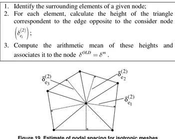
Algorithm 15. Isotropic mesh parameter estimation (see Fig. 19).
1. Identify the surrounding elements of a given node;
2. For each element, calculate the height of the triangle correspondent to the edge opposite to the consider node
( )
( )
i2 e δ ;
3. Compute the arithmetic mean of these heights and
associates it to the node δOLD=δm.
) 2 ( e1 δ ) 2 ( e2 δ ) 2 ( e3 δ
Figure 19. Estimate of nodal spacing for isotropic meshes.
For anisotropic quadrilateral or mixed meshes, we propose a procedure in which the quadrilateral elements are subdivided into triangles (step 1 of Algorithm 14) through their biggest diagonal before the domain is actually remeshed. For the anisotropic triangular meshes, the average nodal values of the mesh parameters are computed as shown in Algorithm 16. Figure 20 presents how to
obtain ( ), ( )
i i
1 2
e e
δ δ and ( )
i
1 e
α in an anisotropic mesh. It must be
error estimate as described previously and with the theoretical knowledge of the a-priori error estimate (Almeida et al., 2000).
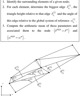
Algorithm 16. Anisotropic mesh parameters estimation (see Fig. 20).
1. Identify the surrounding elements of a given node;
2. For each element, determine the biggest edge ( )
i
1 e δ , the
triangle height relative to that edge ( )
i
2 e
δ and the angle of
this edge relative to the global system of reference ( )
i
1 e α .
3. Compute the arithmetic mean of these parameters and
associated them to the node
(
δOLD=δm)
and(
OLD m)
α =α .
) 1 ( e2
α
) 1 ( e1
α
) 2 ( e1
δ
) 2 ( e3
δ
) 2 ( e2
δ
(1) e1
δ
) 1 ( e2
δ
) 1 ( e3
δ
y
x
Figure 20. Estimate of nodal spacing for anisotropic meshes.
Further Examples
Some extra examples are presented in this section to illustrate some of the flexibilities of the mesh generation methodology and to shown its performance on some CFD computations. Here, we just present the meshes used during these applications. For further details on the different formulations adopted and detailed results of the presented problems see the references listed on each application.
Steady-State Inviscid Flow Simulation with Isotropic Remeshing
A triangular mesh used for the simulation of a supersonic compressible flow around a cylinder, at Mach number of 3.0 and angle of attack of 0° (Lyra, 1994 and Lyra and Morgan, 2002) was used in this example to demonstrate the flexibility for isotropic remeshing. The solution main features consist basically in the front bow shock, the rarefaction zone and the weak shocks behind the cylinder. Figure 21a shows the triangular mesh created by the remeshing procedure. Figure 21b shows a portion of the quadrilateral mesh created with remeshing and originated from the mesh presented in Fig. 21a.
a) b)
Figure 21. a) Triangular mesh around cylinder after remeshing: b) Zoom of quadrilateral mesh around cylinder after remeshing.
Steady-State Inviscid Flow Simulation with Anisotropic Remeshing
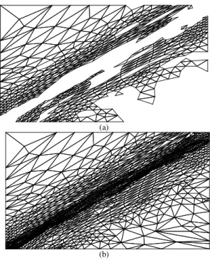
Consider the solution of the inviscid flow problem of regular shock reflection at a flat plate (Lyra and Morgan, 2002). A flow impinging on the plate at a Mach number of 2.0 and at an angle of attack of -10°. The theoretical solution consists of a leading edge reflected shock at 29.3° to the flat plate. A rectangular domain, such that the theoretical shock is positioned at its diagonal, is adopted. In Fig. 22 the final meshes obtained after four stages of global adaptive remeshing is presented for either triangular (Fig. 22a) or quadrilateral (Fig. 22b) elements. The meshes are refined and aligned with the shock. The triangular mesh has 1835 elements and 939 nodes and the quadrilateral mesh has 1377 elements and 1401 nodes. The adaptive strategy is such that the element shape and direction is obtained by requiring that the local error estimative yields the same value in any direction.
(a)
(b)
Figure 23 illustrates the flexibility and robustness of the anisotropic triangular local remeshing procedure. In Figure 23a we plot the remaining elements after eliminating the elements which must change significantly the spacing and/or stretching direction, according to the error analysis. In Figure 23b shows the mesh after the holes are filled by triangles using the advancing front technique. Those meshes correspond to the first local remeshing performed after a global remeshing on the initial mesh.
(a)
(b)
Figure 23. Triangular local remeshing.
Transient Inviscid Flow
Considers the solution of an internal transient inviscid supersonic flow (Lyra et al. 2002). The geometry consists in a wind tunnel with a step and the inflow boundary condition consists of a uniform Mach 3.0 flow with angle of attack 0°. At the right boundary the flow is let free to leave the domain and along the walls, reflecting boundary conditions are applied. During the transient adaptive procedure several adapted meshes are generated along the time integration according to the error analysis. Figure 24 shows some selected meshes: mesh 3, is the third mesh generated during the transient adaptive process, and meshes 20, 27 and 49 are meshes generated before and after the time when the shock starts to be reflected from the top boundary. The mesh refinement is clearly following the physical features of the flow. The adaptive algorithm try to obtain an “optimal” mesh for a pre-defined number of elements. The target number of elements for this analysis was 1000 and a limited aspect ration of 4 was considered. The number of elements generated in the meshes shown was 620, 977, 994 and 1010, and the corresponding number of nodes was 638, 1007, 1029 and 1047, showing that the procedure obeyed well the imposed constraints (Lyra et al. 2002).
Mesh 3
Mesh 20
Mesh 27
Mesh 29
Figure 24. Selected initial meshes for the transient adaptive procedure (Meshes 3, 20, 27 and 29).
Moving Boundary Application
(a)
(b)
(c)
(d)
Figure 25. Local remeshing for problems involving moving meshes: a) mesh without “bad” elements; b) final mesh; c) initial mesh; d) deformed mesh.
Final Remarks and Conclusions
We have briefly described the most important features of a general two-dimensional unstructured mesh generation/adaptation computational methodology, and we also presented some academic examples to illustrate its flexibility and the good quality of the meshes obtained by using it. The main goals during the development stages of the methodology were to keep the strategies simple and ease to implement, and to make possible: to convert any available triangular mesh into a quadrilateral or mixed mesh; to inherit from an available triangular mesh generator the capability for controlling the quality, gradation and stretching of the elements; to retain and extend the flexibility for mesh adaptation through remeshing; to create directional stretched meshes in any portion of the domain. This mesh generator/adapter program opens the possibility to the analyst to choose the best type of element for his formulation and application, and basically whatever can be done with triangles can also be done with quadrilaterals. Some examples of computational fluid dynamics applications have been tackled with our
methodology and were also briefly presented showing that the obtained meshes are valid for numerical simulation. The extension of some of the proposed approaches into three dimensions would require a lot more effort, if possible, and the issue of a robust unstructured hexahedra mesh generator faces many difficulties and represents a very challenging research topic (Thompson et al., 1999 and Carey, 2002).
Acknowledgements
We would like to thank Profs. Morgan, Hassan and Peraire for providing the triangular mesh generator which was the starting point of the whole mesh generation program described in this article. We also gratefully acknowledge the financial support given by the Brazilian agencies CNPq, FINEP and ANP during the execution of this work.
References
Ait-Ali-Yahia, D., Habashi, W. G., Tam, A., Vallet, M.-G. and Fortin, M., 1996, “A Directionally Adaptive Methodology Using An Edge-Based Error Estimate on Quadrilateral Grids”, International Journal for Numerical Methods in Fluids, Vol.23, pp. 673-690.
Almeida, R.C., Feijo, R.A., Galeão, A.C., Padra, C. and Silva, R.S., 2000, “Adaptive Finite Element Computational Fluid Dynamics Using an Anisotropic Error Estimator”, Computer Methods in Applied Mechanics and Engineering, Vol.182, pp. 379-400.
Alquati, E.L.G. and Groehs, A.G., 1995, “Transforming Triangles Into Quadrilaterals for Finite Element Unstructured Meshes”, CILAMCE 95 - XVI Iberian Latin American Conference On Computational Methods for Engineering, Curitiba-Brazil, November, pp. 478-487, (In Portuguese).
Bathe, K.J., 1996, “Finite Element Procedures”, Prentice--Hall, Inc. Blacker, T.D. and Stephenson, M.B., 1991, “Paving: a New Approach to Automated Quadrilateral Mesh Generation”, International Journal for Numerical Methods in Engineering, Vol.32, pp. 811-847.
Borouchaki, H. and Frey, P.J., 1998, “Adaptive Triangular-Quadrilateral Mesh Generation”, International Journal for Numerical Methods in Engineering, Vol.41, pp. 915-934.
Carey, G.F., 2002, “Hexing the Tet.” Communications in Numerical Methods in Engineering, Vol.18, No. 3, pp. 223-227.
Gendong, C. and Li, H., 1996, “New Method for Graded Mesh Generation of Quadrilateral Finite Elements”, Computers and Structures, Vol.59, pp. 823-829.
George, P.L., 1991, “Automatic Mesh Generation: Application to Finite Element Methods”, Wiley, New York, USA, 344 p.
Hassan, O., Morgan, K., Peraire, J., Probert, E.J. and Thareja, R.R., 1991, “Adaptive Unstructured Mesh Methods for Steady Viscous Flow”, AIAA-91-1538.
Hassan, O., Probert, E.J., Morgan, K. and Peraire, J., 1993a, “Adaptive Finite Element Methods for Transient Compressible Flow Problems”, In: Proceedings “Adaptive Finite and Boundary Element Methods'', CML Publications, pp. 119-160.
Hassan, O., Probert, E.J., Morgan, K. and Peraire, J., 1993b, “Line Relaxation Methods for the Solution of 2-D and 3-D Compressible Viscous Flows Using Unstructured Meshes”, In: Proceedings “Recent Developments and Applications in Aeronautical CFD”, Royal Aeronautical Society, Bristol, pp. 7.1-7.11, Bristol.
Hassan, O., Probert, E.J., Weatherill, N.P., Marchant, M.J., Morgan, K. and Marcum, D. L., 1994, “The Numerical Simulation of Viscous Transonic Flow Using Unstructured Grids”, AIAA-94-2346.
Hwang, C.J. and Wu, S.J., 1992, “Global and Local Remeshing Algorithms for Compressible Flows”, Journal of Computational Physics, Vol.102, pp. 98-113.
Jansen, K.E and Shephard, M.S., 2001, “On Anisotropic Mesh Generation and Quality Control in Complex Flow Problems”, In: Proceedings, 10th International Meshing Roundtable, pp. 341-349.
Knupp, P.M., 2003, “Algebraic Mesh Quality Metrics For Unstructured Initial Meshes”, Finite Elements in Analysis and Design, Vol.39, pp. 217-241.
Lee, K-Y., Kim, I-I, Cho, D-Y and Kim, T-W, 2003, “A algorithm for 2D Quadrilateral Mesh Generation With Line Constraints”, Computers-Aided Design, pp. 1-14.
Lyra, P.R.M., 1994, “Unstructured Grid Adaptive algorithms for Fluid Dynamics and Heat Conduction”, Ph.D. thesis, University of Wales – Swansea.
Lyra, P.R.M., de Carvalho, D.K.E. and Willmersdorf, R.B., 1998, “Adaptive Triangular, Quadrilateral and Hybrid Unstructured Mesh Generation With Classical Resequencing Techniques”, WCCM'98 - Proc. of the 4th World Conference on Comput. Mechanics, Buenos Aires/Argentina, June, published In CD-ROM.
Lyra, P.R.M. and de Carvalho, D.K.E., 2000, “A Flexible Unstructured Mesh Generator for Transient Anisotropic Remeshing”, ECCOMAS 2000 - European Congress on Computational Methods in Applied Sciences and Engineering 2000, Barcelona-Spain, September, pp.1-19, published in CD-ROM.
Lyra, P.R M., Almeida, F.P.C., Willmersdorf, R.B. and Afonso, S.M.B., 2000, “An Adaptive FEM Integrated System for the Solution of Transient Thermal-Structural Problems”, CILAMCE 2000 - Iberian Latin American Congress on Computational Methods in Engineering, Rio de Janeiro-Brazil, December, In CD-ROM.
Lyra, P.R.M., de Carvalho, D.K.E., Pereira de Carvalho, R. M. and Almeida, R.C.C., 2001, “Finite Element Compressible Flow Computation Using a Transient Anisotropic Remeshing Procedure”, ECCOMAS Computational Fluid Dynamics 2001 Conference, Swansea-UK, September, In CD-ROM.
Lyra, P.R.M., de Carvalho, D.K.E., Willmersdorf, R.B. and Almeida, R.C.C., 2002, “Transient Adaptive Finite Element Analysis of Compressible Flows”, WCCM'2002 - Proceedings of the 5th World Conference on Computational Mechanics, Vienna-Austria, July, (Proceedings on http://wccm.tuwien.ac.at/).
Lyra, P.R.M. and Antunes A.R.E., 2002, “The Analysis of Fluid-Structure Interaction Using an ALE Finite Element Formulation”, GIMC 2002 - Proc. of the Third Joint Conference of Italian Group of Computational Mechanics and CILAMCE 2002 - Iberian Latin American Congress on Computational Methods in Engineering, pp. 1-10, In CD-ROM.
Lyra, P.R.M. and Morgan, K., 2002, “A Review and Comparative Study of Upwind Biased Schemes for Compressible Flow Computation. Part III: Multidimensional Extension on Unstructured Grids, Archives of Computational Methods in Engineering, Vol.9, No. 3, pp. 207-256.
Lyra, P.R.M. Almeida, R. C., 2002, “A preliminary study on the performance of stabilized finite element CFD methods on triangular, quadrilateral and mixed unstructured meshes.”, Communications in Numerical Methods in Engineering, Vol.18, No. 1, pp. 53-61.
Marcum, D.L., 1995, “Generation of Unstructured Grids for Viscous Flow Applications”, In: 33rd Aerospace Sciences Meeting and Exhibit, AIAA-95-0212.
Peiró, J.,1989, “A Finite Element Procedure of the Euler Equations on Unstructured Meshes”, Ph.D. thesis, Department of Civil Engineering, University – Swansea.
Peiró, J., Peraire, J. and Morgan, K., 1994, “{FELISA SYSTEM}: Reference Manual Part1 - Basic Theory”, University of Wales Swansea Report CR/821/94.
Peraire, J., Vahdati, M., Morgan, K. and Zienkiewicz, O.C., 1987, “Adaptive Remeshing For Compressible Flow Computations”, Journal of Computational. Physics, Vol.72, pp. 449-466.
Rippa, S., 1992, “Long and Thin Triangles Can Be Good for Linear Interpolation”, SIAM Journal of Numerical Analysis, Vol.29, pp. 257-270.
Sarrate, J., Gutiérez, M.A. and Huerta, A., 1993, “A New Algorithm for Unstructured Quadrilateral Mesh Generation and Rezoning”, In: Finite Elements in Fluids, Pineridge Press, pp. 745-754.
Schroeder, W.J. and Shephard, M.S., 1990, “A Combined Octree/Delaunay Method for Fully Automatic 3-D Mesh Generation”, International Journal for Numerical Method in Engineering, Vol.29, pp. 2005-2039.
Secchi, S. and Simoni, L., 2003, “An Improved Procedure for 2D Unstructured Delaunay Mesh Generation”, Advances in Engineering Software, Vol.34, pp. 217-234.
Thompson, J.F., Soni, B.K. and Weatherill, N.P., 1999, “Handbook of Grid Generation”, CRC Press, 1200 p.
Xie, G. and Ramaekers, J.A.H., 1994, “Graded Mesh Generation and Transformation”, Finite Elements in Analysis and Design, Vol.17, pp. 41-55. Weatherill, N.P., 1990, “Mesh Generation In Computational Fluid Dynamics”, Von--Karman Institute for Fluid Dynamics Lecture Notes, 1990-10.